Article

A Study of Machine Learning Regression Techniques for Non-Contact SpO2 Estimation from Infrared Motion-Magnified Facial Video

by
Thomas Stogiannopoulos
,
Grigorios-Aris Cheimariotis
and
Nikolaos Mitianoudis
*,†
Electrical and Computer Engineering Department, Democritus University of Thrace, 67100 Xanthi, Greece
*
Author to whom correspondence should be addressed.
These authors contributed equally to this work.
Information 2023, 14(6), 301; https://doi.org/10.3390/info14060301
Submission received: 18 April 2023 / Revised: 16 May 2023 / Accepted: 17 May 2023 / Published: 23 May 2023
(This article belongs to the Section Biomedical Information and Health)

Abstract

:
This work explores the use of infrared low-cost cameras for monitoring peripheral oxygen saturation (SpO2), a vital sign that is particularly important for individuals with fragile health, such as the elderly. The development of contactless SpO2 monitoring utilizing RGB cameras has already proven successful. This study utilizes the Eulerian Video Magnification (EVM) technique to enhance minor variations in skin pixel intensity in particular facial regions. More specifically, the emphasis in this study is in the utilization of infrared cameras, in order to explore the possibility of contactless SpO2 monitoring under low-light or night-time conditions. Many different methods were employed for regression. A study of machine learning regression methods was performed, including a Generalized Additive Model (GAM) and an Extra Trees Regressor, based on 12 novel features extracted from the extracted amplified photoplethysmography (PPG) signal. Deep learning methods were also explored, including a 3D Convolution Neural Network (CNN) and a Video Vision Transformer (ViViT) architecture on the amplified forehead/cheeks video. The estimated SpO2 values of the best performing method reach a low root mean squared error of 1.331 and an R 2 score of 0.465 that fall within the acceptable range for these applications.

1. Introduction

Tracking vital signals, such as SpO2, which measure the level of oxygen in the blood, is important in countries with a large geriatric population for several reasons. First and foremost, older adults are more susceptible to chronic health conditions, such as cardiovascular disease [1], chronic obstructive pulmonary disease (COPD) [2], and sleep apnea [3], all of which can affect oxygen saturation levels. Monitoring SpO2 can help identify early warning signs of these conditions, allowing for timely intervention and management. For example, low oxygen saturation levels can indicate that an individual is not getting enough oxygen to their body, which can be a sign of a serious condition, such as COPD [4] or sleep apnea [5]. Secondly, changes in oxygen saturation levels can also indicate the presence of other health issues, including infections, anemia, and even cancer [6]. Monitoring these signals can help detect these issues early on, when they are more treatable and provide a more holistic view of the individual’s health. Lastly, in countries with a large geriatric population, there is a growing need for remote monitoring solutions to help manage the healthcare of older adults. In this paper, the focus is on exploring the potential of non-contact methods to estimate peripheral oxygen saturation (SpO2) utilizing data retrieved from an infrared camera. As far as our knowledge and research shows, there have not been any previous attempts or studies aimed at estimating SpO2 without physical contact using an infrared camera, lacking an external infrared light source. The motivation behind using infrared cameras is that there might be cases during the evening or night-time, where common RGB cameras cannot offer any significant image quality due to low light levels. Using infrared cameras, systems can continue monitoring people’s vital signs remotely during their sleep, without the need to attach monitoring sensors to patients.
Peripheral oxygen saturation (SpO2) refers to the percentage of oxygenated hemoglobin in the blood, compared to the total amount of hemoglobin present [7,8]. It is an important clinical measurement used to evaluate a person’s oxygenation status, which is a crucial factor in many physiological processes and can impact overall health. A normal SpO2 reading is typically between 96 and 100% [7], with lower values indicating a lack of adequate oxygen delivery to the body’s tissues. Peripheral oxygen saturation (SpO2) is mathematically defined as [8]
S p O 2 = H b O 2 H b O 2 + H b × 100 %
where H b is the de-oxygenated hemoglobin and H b O 2 is the oxygenated hemoglobin. The measurement is typically taken using a pulse oximeter. This device works by shining two different wavelengths of light, usually red and infrared [9], through the skin and into the blood vessels of a peripheral body part, such as a finger or earlobe. The light passing through the blood absorbs and scatters differently, based on the presence of oxygenated and deoxygenated hemoglobin. The pulse oximeter measures the amount of light absorbed at each wavelength and calculates the SpO2 value based on the ratio of the absorbed light.
Unfortunately, direct skin contact with the patient is necessary for pulse oximetry measurement, and this is not always possible due to their relatively invasive nature, time-consuming procedures, sources of error, and high costs. These factors render oximeters less desirable options for monitoring SpO2. Non-contact techniques for measuring vital signs effectively address the previously mentioned challenges [10,11,12]. These studies opened up opportunities for new advancements, such as image photoplethysmography (iPPG) and remote photoplethysmography (rPPG), i.e., contactless techniques for monitoring blood volume changes in the microvascular bed of human tissue. Image photoplethysmography involves the use of cameras and imaging systems, such as Laser Speckle Contrast Imaging (LSCI) [13]. The camera works by shining a laser onto a sample and measuring the intensity fluctuations, caused by red blood cells moving through the tissue [14,15]. Later, it sends the data off for offline processing, which can be analyzed to determine the blood volume changes. Remote photoplethysmography, on the other hand, involves the use of light-emitting diodes (LEDs) or other light sources that are placed at a distance from the tissue, and the changes in light reflection or transmission are measured by a remote photodetector. The data collected by the photodetector is then used to calculate the changes in blood volume [16]. In [17], Akamatsu et al. use RGB camera inputs to predict the heart rate and SpO2 levels using motion amplification and a deep-learning approach.
Eulerian Video Magnification (EVM) is a technique, proposed by Wu et al. [18], in order to amplify and thus make visible very small motions, captured by current RGB cameras, that are normally invisible to the human eye. When applied to image photoplethysmography, Eulerian Video Magnification (EVM) can enhance the accuracy and sensitivity of the measurement of oxygen saturation (SpO2) levels. This is due to the fact that the EVM technique can detect even the slightest changes in skin blood flow [18], providing a more detailed and precise measurement of oxygen saturation, or the patient’s physiological state in general, allowing for better monitoring and treatment of medical conditions. Thus, in this paper, we propose the use of EVM, as a preprocessing step to enhance the video content captured by the infrared camera. Recent research has explored and demonstrated various methods for estimating oxygen saturation levels using facial video with multimodal physiological data generation [19] or via DC and AC component extraction of a spatio-temporal map using facial videos [17].
The aim of this work is to evaluate the feasibility of using infrared single-channel videos for the accurate and efficient estimation of SpO2. The motivation behind this investigation is the potential advantages of using single-channel infrared videos, including reduced computational complexity and lower hardware requirements that can be used to inform the design and development of future SpO2 estimation systems. Additionally, our study shows that the proposed SpO2 estimation methodology using feature extraction performs better than the state-of-the-art SpO2 estimation methods previously established by Akamatsu et al. [17].

2. Dataset Protocol and Equipment

In order to assess the performance of the proposed method for estimating peripheral oxygen saturation (SpO2), a dataset of infrared facial videos with SpO2 measurements was created. Twenty one (21) participants took part in two experiments each. To ensure a relaxed and calm state, it was decided that each subject would be monitored for two (2) minutes. The reference point for each participant’s oxygen saturation was a commercial pulse oximeter (JPD-500D ControlBios Oxicore Pulse Oximeter) that tracked the SpO2 levels continuously during the 2 min trials. Some of the subjects were recorded in a dark room, while the rest were filmed in a room with natural sunlight using an infrared camera. The participants were instructed to remain as still as possible for 2 min during each recording. During the first video recording, they were asked to breathe normally and during the second recording, they were asked to hold their breath as much and as long as they felt comfortable, in order to capture lower SpO2 levels. To avoid potential registration issues, the participants were seated at a fixed distance from the camera.
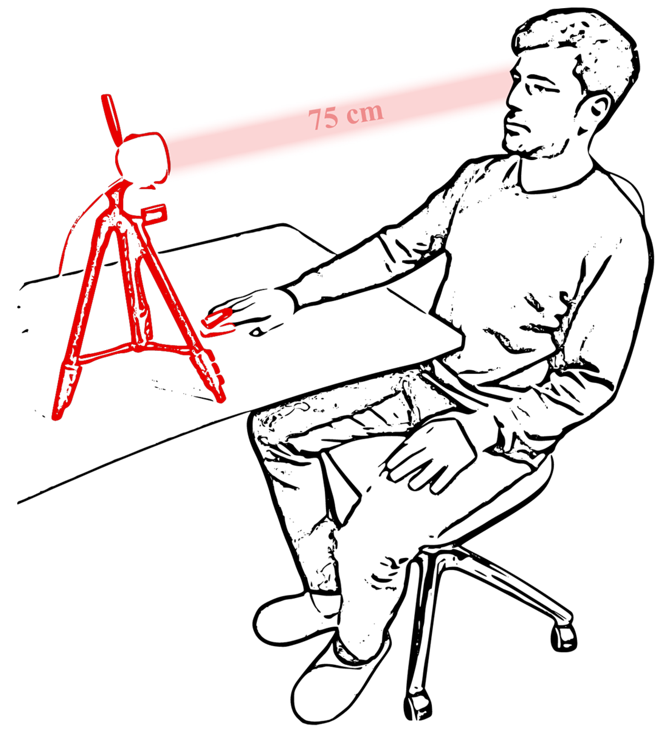
The authors used a wired Google Nest Cam to capture the videos of the participants. The camera was set to “Infrared Always” mode and had a resolution of 1920 × 1080 Full HD. The frame rate of the camera was 30 fps. The camera was placed at eye level, 75 cm away from the participants, to minimize any distortion that might have been caused by the wide-angle lenses of the camera. The video clips were processed from the surveillance stream by first downloading them from Google’s Cloud service, where they were uploaded. It is crucial to keep in mind that the video clips contained a significant amount of compression noise, which had the potential to affect the accuracy of the facial feature extraction process. Thus, we had to work with the compressed video clips that were available through the Google Cloud service, since direct extraction of the raw sensor data was not possible with the current software provided by Google. The main aim of this practice was to demonstrate the feasibility of the proposed approach, even with lower-end commercial equipment, as opposed to more high-end cameras with higher resolution or frame rate that would not be easily available to an average home user. Despite the considerable amount of compression noise, the proposed approach managed to produce satisfactory results that can validate our proof of concept.

3. Proposed Methodology

The proposed methodology consists of mainly four steps. Figure 1 depicts a flowchart of the proposed system. The first step entails the detection of the face and extracts the desired facial areas for the procedure. The second step includes the motion magnification step. During the third step, we extract the proposed features from the desired facial regions. In the final step, the extracted features or the extracted regions are presented to a traditional machine learning or a deep learning regression system that predicts the SpO2 index. In the following sections, these steps will be analysed in more detail.
The proposed methodology consists of four steps:
  • Detect the face and extract the desired facial areas for the procedure.
  • Apply motion magnification.
  • Extract the proposed features from the desired facial regions.
  • The extracted features or the extracted regions are presented to a traditional machine learning or a deep learning regression system that predicts the SpO2 index.
In order to provide a clear and concise representation of our methodology, we have created a flowchart in Figure 1 that summarizes the various steps involved in our SpO2 estimation approach. In the following sections, these steps will be analysed in more detail. It should be stressed that Figure 1 outlines the conducted experiments, which implies that both traditional machine learning and deep learning methods were tested for regression. The system does not use both machine and deep learning regression algorithms simultaneously.

3.1. Facial Segmentation

The facial area was deliberately selected for the estimation of SpO2, with a focus on the forehead and the left and right cheek regions. The high levels of blood flow in the facial regions would provide more accurate and reliable SpO2 readings. Additionally, the forehead and cheeks are easily accessible for both men and women. One should also consider the fact that the jaw, lips and chin areas may be covered with facial hair in men, rendering them difficult to use for monitoring purposes. The method employed in this research involves utilizing 2 min video clips recorded from an infrared camera as input. At first, the Viola–Jones algorithm [20] is employed to detect the face in the 2 min video clip and then, the next step is to isolate and identify the specific regions of the forehead and the left/right cheek in the detected face. This is accomplished employing some standard ratios between standard face landmarks in the average human face, as discussed in more detail in [21,22,23].
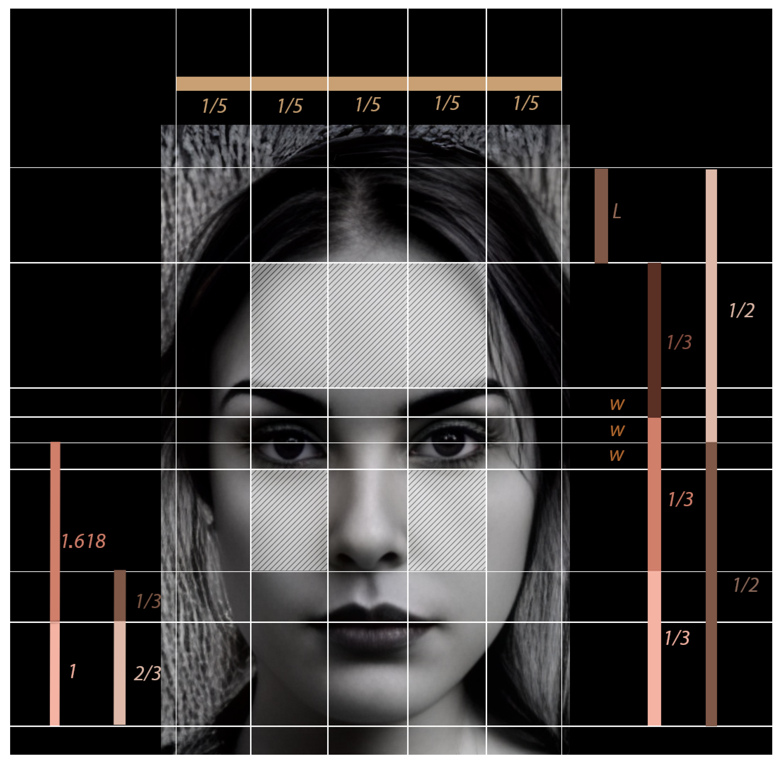
Figure 2 depicts the required information about the average human face, in order to estimate the coordinates of three rectangular regions containing the forehead, and the left and right cheek. In the most likely scenario, the bounding box, generated by the Viola–Jones algorithm, would encompass a rectangular region extending from one ear to the other, and from the forehead to the chin, encapsulating the entire face. Assuming that the identified rectangular area is actually a square, this simplifies the calculations involved in determining the accurate coordinates of the desired regions of interest. This simplification also reduces the computational cost during the ROI video frame sequence extraction process. Let X and Y represent the distances from the chin to the top of the head and the chin to the forehead respectively, constant ϕ is the golden ratio, and W represents the width of the facial segments that needs to be subtracted in order to eliminate extraneous features, such as the eyebrows and eyes. Following Figure 2, it is straightforward to derive the following two equations:
2 Y 3 = X 2 + W
X 2 = 2 Y 9 ( 1 + ϕ )
The value of W can then be determined, as follows:
W = 2 Y 9 ( 2 ϕ ) = 2 Y 9 ( 2 1 2 5 2 ) = Y ( 1 3 5 9 )
Since the value of Y will be known from the bounding box, determined by the Viola–Jones algorithm, the desired regions of interest can now be accurately cropped. This allows for successful isolation of these regions and subsequent analysis of their photoplethysmographic signals.
It should be noted that the Viola–Jones algorithm may be sensitive to factors such as camera angle and position of the head with respect to the camera. However, we make the assumption that the participant’s head is facing the camera straight at their eye level, 75 cm away, as this was the setup during the experiment. This assumption is made in order to simplify the facial segmentation process and avoid dealing with the complexities that may arise from varying camera angles and head positions. Figure 3 depicts the experimental setup that was used during data acquisition. This setup was fixed for all subjects, therefore, minimising the risk of face identification and registration errors. The examination of the signal processing techniques used in this study will be presented in depth in the following section.

3.2. Motion Magnification

The subsequent step involves the application of the Eulerian Video Magnification method, as proposed by Wu et al. [18], with the purpose of enhancing the signals of the blood flow in the facial regions, as captured by the infrared camera. This was achieved by magnifying the subtle variations in the intensity of the infrared light, due to the changing blood flow, by setting the amplification factor to α = 120 . Assuming a small invisible movement δ ( t ) at pixel r = ( x , y ) of the original video sequence V ( x , y , t ) , the motion magnification approach attempts to magnify the movement and produce the magnified video sequence I ( x , y , t ) , as follows:
I ( r , t ) = V ( r , t ) + α B ( r , t ) f ( r + ( 1 + α ) δ ( t ) )
Wu et al. [18] perform a Laplacian pyramid decomposition for each frame and the motion amplification is performed along the time axis t. The concept can be extended for multiple frequencies, where we can select a range of motion frequencies that can be amplified by the framework. The frequency range of amplification for this application was carefully chosen to be between 0.4 and 4 Hz. This frequency range encompasses the typical human heart rate range, even in instances where the heart rate can increase to an extremely high rate (supraventricular tachycardia—SVT), reaching a peak of 240 beats per minute (bpm), according to Garratt et al. [24]. In their study, Kong et al. [8] employed a frequency range that was similar to the one used in the present work, to amplify the blood flow signals in their experiments. In order to decrease the computational cost of the proposed approach, motion magnification is performed only to the three extracted facial areas and not to the whole face.
Eulerian Video Magnification (EVM) is a powerful tool for visualizing subtle temporal variations in videos that are difficult or impossible to perceive with the naked eye. EVM has been successfully used in a variety of applications, including extracting vital physiological information from videos of human faces [10,25] and animals [26].

3.3. Feature Extraction

Several unique features that are inherently associated with the statistical characteristics of the iPPG signal can be derived from the three targeted areas of interest. These features could provide valuable insights and contribute to a better understanding of the iPPG signal. Some basic statistical measurements for this task were proposed in [8,10]. More specifically, in [8,10] the mean value and standard deviation of two color channels were employed as features from one facial region. In our case, we use a single IR channel and three facial regions. Due to the limited information provided by the single channel, we investigated the use of combinations of spatial and temporal statistics (mean and standard deviation) from all three regions. In essence, we concentrate our analysis on four distinct features that can be derived from the intensity values of the single-channel video frames. Assume that a sequence of motion-magnified frame sequence I i ( x , y , t ) , where i = 1 , 2 , 3 represents each of the three facial areas, x , y are the spatial coordinates and t the frame index. The proposed features F j i are given by the following:
  • The mean of the average intensity of all frames:
    F 1 i = mean t { mean x , y { I i ( x , y , t ) } }
  • The standard deviation of the average intensity of all frames:
    F 2 i = std t { mean x , y { I i ( x , y , t ) } }
  • The mean of the standard deviation of the intensity of all frames:
    F 3 i = mean t { std x , y { I i ( x , y , t ) } }
  • The standard deviation of the standard deviation of the intensity of all frames:
    F 4 i = std t { std x , y { I i ( x , y , t ) } }
In summary, we estimate four different combinations of mean values and standard deviation over spatial or temporal axes. In total, the extraction of four features for each of the three regions of interest results in a total of twelve features. These extracted features, which have been proposed in this work, will be utilized as inputs for traditional machine learning regression algorithms in the upcoming section.

4. Machine Learning Regression

Previous studies [8,10,25] have utilized multiple colour channels and traditional methodologies, which enabled them to fine-tune their models by performing simple linear regression. However, our study differs in that we utilized a single colour channel and concluded that linear regression was insufficient for accurately modeling our data. Therefore, we had to explore additional regression algorithms, including Neural Networks, to achieve an acceptable level of accuracy in our model. This highlights the importance of carefully selecting appropriate methodologies based on the specific characteristics of the dataset and the research question at hand, rather than relying on standard approaches used in previous studies.

4.1. Traditional Techniques

Machine learning techniques have also sought to perform regression, i.e., prediction of an output value, based on a set of input values. Therefore, many techniques have been proposed in the past. In this study, we tested a number of these techniques that were included in the popular scikit-learn Python library. We used the twelve proposed features as input to the these regression techniques and the output value was the measured SpO2. The techniques that were used were the following: Linear regression, Ridge regression, SGD Regressor, ElasticNet, Lars, Lasso, LassoLars, Huber Regressor, Quantile Regressor, RANSAC Regressor, Theilsen Regressor, Poisson Regressor, Tweedie Regressor, Gamma Regressor, AdaBoost Regressor, Bagging Regressor, Extra Trees Regressor, HistGradient Boosting Regressor, Gradient Boosting Regressor, and Random Forest Regressor. The full list of regression models that were used in the present study is presented in detail in Table 1, where the parameters for each technique are depicted.

4.2. Generalized Additive Model

Generalized Additive Models (GAMs) are a type of regression model that allow for the modeling of non-linear relationships between a response variable and one or more predictor variables [27]. They are well suited for regression tasks, because they are able to capture more complex relationships in the data compared to traditional linear regression models, such as Generalized Linear Models (GLMs). GLMs are used to model linear relationships between a response variable and one or more predictor variables, but they have limitations in capturing non-linear relationships in the data. GLMs also assume a specific distribution for the response variable, such as a normal or Poisson distribution, which may not always be appropriate for the data [28]. To overcome these limitations, Additive Models were introduced, which allow for the modeling of non-linear relationships by summing up multiple functions of the predictor variables (basis functions). In addition, they do not make assumptions about the distribution of the response variable and can handle a wider range of response variable distributions. A GAM can mathematically represent the relationship between a random variable Y and a series of predictor random variables X 1 , X 2 , , X p through their summation, as follows:
E { Y | X 1 , X 2 , , X p } = f 0 + j = 1 p f j ( X j )
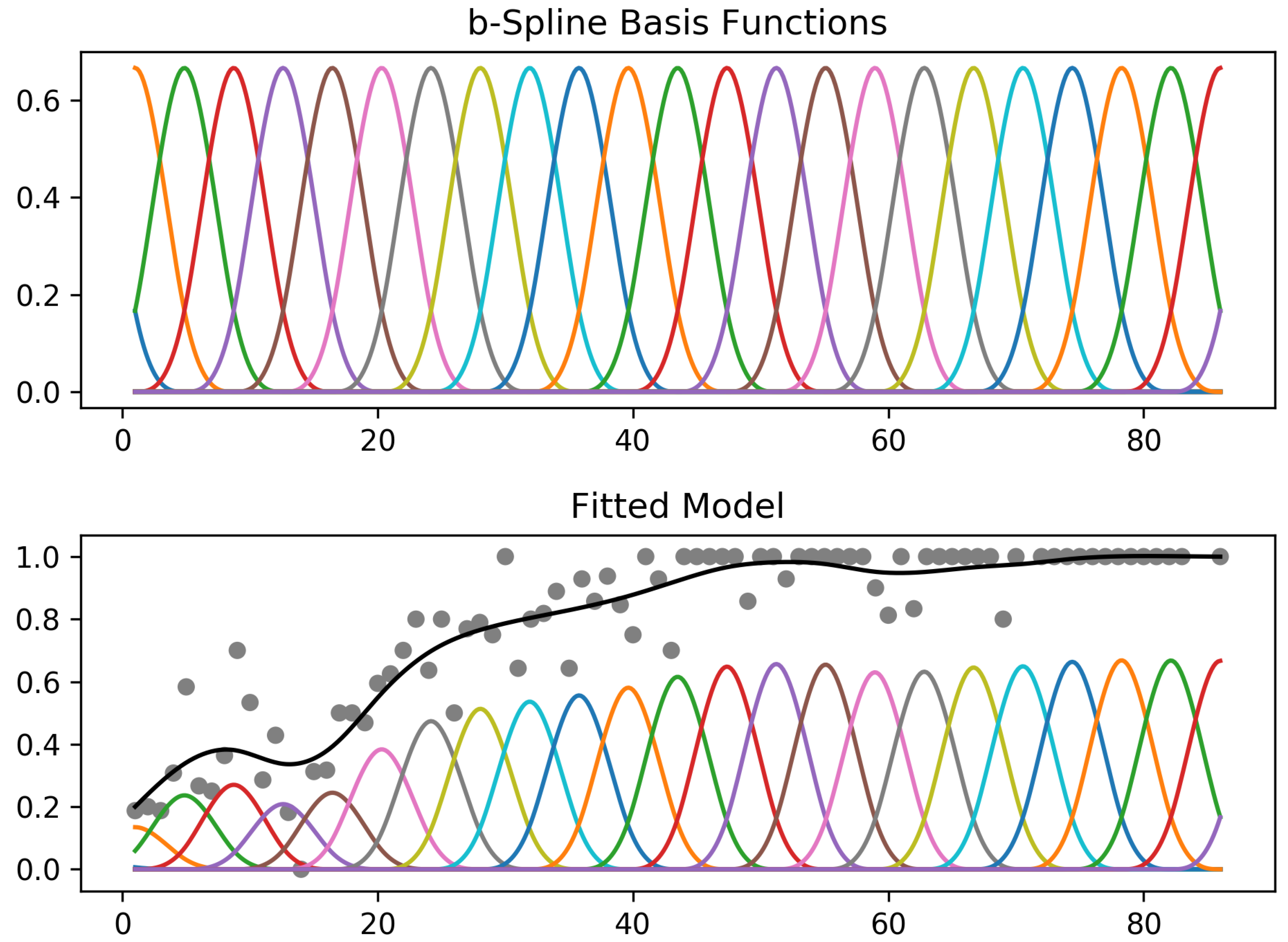
where f j ( · ) are smooth nonparametric standardized functions, so that E { f j ( X j ) } = 0 [27] and E { · } refers to the expectation operator. Overall, Generalized Additive Models are a more flexible and powerful tool for regression tasks, compared to Generalized Linear Models, especially when dealing with complex, non-linear relationships in the data. Figure 4 is an illustration of a Generalized Additive Model (GAM).
The choice of the number of splines in a GAM is typically determined by a trade-off between model complexity and goodness of fit. A smaller number of splines can lead to a more parsimonious model, but may result in underfitting, while a larger number of splines can increase the model’s complexity and may result in overfitting. In this study, the number of splines in the linear GAM model was chosen, based on prior knowledge and assumptions about the complexity of the underlying relationships between the predictor variables and the response variable, as well as on the available sample size and computational resources. In this study, to determine the optimal number of splines for the Generalized Additive Models, we conducted multiple experiments with varying numbers of splines. This was carried out to evaluate the impact of the number of splines on the accuracy of the models.

4.3. Extremely Randomized Trees

The Extra Trees Regressor (ETR) is a type of ensemble-based machine learning algorithm that can be used for both classification and regression tasks [30]. The ETR is based on the decision tree algorithm, but it combines multiple decision trees to improve prediction accuracy. The “Extra” in the Extra Trees Regressor refers to the fact that this algorithm uses an extra layer of randomness, compared to other decision tree-based algorithms. Specifically, the ETR randomly selects a subset of features for each split in the decision tree, and it also randomly selects the threshold for each feature. This randomness helps to create a more diverse set of decision trees and reduce overfitting, which can improve prediction accuracy. The ETR is also an example of a bagging ensemble method, which means that it trains multiple models on different subsets of the training data and combines their predictions to make a final prediction [30]. In the case of the ETR, the algorithm trains multiple decision trees on different subsets of the training data and combines their predictions by taking the average of the predicted values. Another advantage of the ETR is its relatively low variance, compared to other ensemble-based methods, such as Random Forest. This means that the ETR is less sensitive to changes in the training data and can often achieve better performance and higher accuracy than other ensemble-based methods. The ETR has several tunable hyperparameters that can be optimized to improve performance, including the number of trees, the maximum depth of the decision trees, and the number of features to consider for each split. The ETR can also be trained faster than other ensemble-based methods due to its simpler decision tree construction and feature selection process [30]. Overall, The Extra Trees Regressor is a powerful machine learning algorithm that can achieve high accuracy in a variety of regression and classification tasks, particularly when the training data is limited or noisy.

5. Deep Learning Regression

5.1. Multilayer Perceptron

For the purposes of this paper, we used a type of Artificial Neural Network, known as a multilayer perceptron. This type of network is characterized by its ability to learn complex non-linear relationships between inputs and outputs, making it well-suited for a variety of regression and classification tasks. Table 2 provides a detailed representation of the architecture for a relatively simple Artificial Neural Network (ANN). The architecture outlines the specific design and configuration of the network, including the number of layers, number of nodes, activation functions, dropout rates, and other important components. Although, it is a fully connected network, it is considered a deep learning network, since it features four (more than two) hidden layers. This architecture is the proposed design for the ANN that will be used in the experimental section, and it has been carefully selected after extended experimentation. The objective is to create an ANN that is capable of accurately modeling the relationship between the input variables and the target variable. The loss function used in this model was the mean squared error, which was optimised using the Adam Optimizer [31] with a learning rate of η = 0.001 , batch size = 5, and 40 epochs. The weights were initialized using He uniform initialization [32]. The name for the proposed ANN architecture is OxygeNN.

5.2. Spatial 3D Convolutional Neural Network

3D-CNNs have been widely used by the vision community for video classification [33], as well for super-resolution scaling in videos [34]. Thus, they have been a popular choice for video classification and regression. In this application, we propose to use a 3D-CNN architecture for predicting the SpO2 level based on the forehead motion-magnified video.
The proposed architecture for the 3D-CNN is presented in Table 3. The depth of this architecture is intentionally kept shallow with the aim of avoiding overfitting and retaining accuracy. By keeping the depth of the 3D-CNN shallow, the model is less likely to overfit, resulting in a more accurate representation of the data patterns. Additionally, a shallower architecture also results in faster training, and prediction, rendering the approach more computationally efficient [35]. It is worth mentioning that in this case, we did not use the proposed 12 features, as previously, but the magnified video I 1 ( x , y , t ) of the forehead as input. There was also a variation of the 3D-CNN developed by incorporating feature fusion. Feature fusion is a technique that combines features from multiple sources, in this case, the magnified videos I 1 ( x , y , t ) , I 2 ( x , y , t ) , I 3 ( x , y , t ) of all regions of interest (ROIs) as inputs for the 3D-CNN. The fusion of features from multiple sources can improve the performance of the model by providing additional information and reducing the impact of noise and irrelevant features [36]. In the application of a Convolutional Neural Network (CNN), the network is able to determine, through the learning process, which features are more significant in order to infer the value of the SpO2. This process of feature selection is carried out through the utilization of filters and weights, which are optimized during the training process, allowing the network to identify relevant patterns and relationships between the input features and the target variable. Allowing the network to perform feature extraction in this manner helps to reduce the dependence on prior knowledge or man-made feature selection, thus exploring new solutions and maybe improving performance in the estimation of SpO2. The loss function used in this model was the mean squared error, which was optimised using the Adam Optimizer [31] with a learning rate of η = 0.001 , batch size = 5 and 100 epochs. The weights were initialized using He uniform initialization [32].

5.3. Video Vision Transformer—ViViT

The Video Vision Transformer (ViViT) is a type of Deep Neural Network architecture that is specifically designed for video-related tasks, such as classification [37]. It is inspired by the Vision Transformer (ViT) architecture that was originally developed for image and vision-related tasks [38], but it has been adapted to work with video data as input. It extends the original Transformer architecture by incorporating spatio-temporal attention, which allows the network to attend to both spatial and temporal aspects of the input. The input is typically first transformed into a set of embedding tokens. These tokens are vectors that represent the input in a high-dimensional feature space, and they are used as the input to the self-attention mechanism. The self-attention mechanism allows the network to attend to different regions of each frame and to different frames in the sequence, enabling it to capture both spatial and temporal relationships between the regions. In order to achieve this, Arnab et al. [37] performed “Uniform Frame Sampling”, using the same method as ViT, and “Tubelet Embedding”, an additional method to extract non-overlapping, spatio-temporal “tubes” from the video volume. The use of smaller tubelets in the tokenization process results in an increase in the number of tokens, which in turn leads to a higher computational cost [37]. This approach of tokenization fuses the spatio-temporal information during the tokenization step. In this work, we utilized a previous implementation of ViViT, developed by Gosthipaty and Thakur [39], for video classification as a starting point for our study. The modification were firstly aimed at changing the loss function in order to transform the original classification architecture to an architecture that can perform regression. Again, in this case, we used the magnified video I 1 ( x , y , t ) of the forehead, instead of the proposed 12 features. More specifically, the current model employs the mean squared error as loss function, optimised using the Adam Optimizer [31] with a learning rate of η = 10 4 , 40 epochs, and a weight decay of λ = 10 5 .

6. Results

6.1. Implementation

Face detection, facial areas extraction and motion magnification were performed in MATLAB R2018b, mainly because the original motion magnification code by Wu et al. [18] was written in MATLAB. The proposed machine learning regression approaches were implemented in Python v3.8.10 using the scikit-learn package. The deep architectures were developed in Python v3.8.10 and Tensorflow v2.10.0. For the experiments, we used an Ubuntu 22.04 PC with 64 GB RAM, an Intel i9 2.5 GHz 16-Core CPU and an NVIDIA GeForce RTX 3090 GPU with 24 GB of RAM.

6.2. Accuracy

The accuracy of pulse oximeters is an important aspect that has been rigorously defined by international organizations, such as the International Organization for Standardization (ISO) and the Food and Drug Administration (FDA) [40,41]. These guidelines and standards specify the acceptable error limits, and they are used by manufacturers, medical facilities, and healthcare providers to ensure that pulse oximeters perform within acceptable limits. The BS EN ISO 80601-2-61:2019 standard states that the root mean square accuracy, which represents the deviation of the measurement from the true value, must not exceed 2% of the SpO2 range [40]. Alternatively, the mean square error, which measures the average difference between the estimated and actual values, must not exceed 4% for a set of testing pair values. The accuracy is defined as the root mean square difference between the estimated values S p O 2 i and reference values S R i and is given by
A r m s = M S E = i = 1 n ( S p O 2 i S R i ) 2 n
where n is the number of samples, S p O 2 i is the calculated value of the i-th sample, and S R i is the reference value for the i-th sample. The threshold of accuracy specified by BS EN ISO 80601-2-61:2019 with regard to the root mean square accuracy not exceeding 2% of SpO2 range, is also recognized and agreed upon by the U.S. Food and Drug Administration (FDA) [41].
While international organizations neither require nor specify additional accuracy criteria for these types of studies, we included additional metrics such as mean absolute error, mean absolute percentage error, and R 2 to provide a more complete picture of our model’s accuracy and to allow for comparison with other similar studies.

6.3. Model Comparison and Selection

In this work, we leveraged the versatility and predictive power of the multilayer perceptron to gain insights into our data and to make informed predictions about our target variable, which was the SpO2 level recorded by the oximeter. To achieve this, the input to the machine learning model were the twelve previously discussed features that were extracted from the iPPG signal in the three regions of interest. These features were used to predict the SpO2 value and were considered as the predictor variables in the regression analysis. In our experiments, we considered all possible combinations of the 12 iPPG-based features, the total number of feature combinations that utilized two or more features per combination being 4083. This is because not all features may have the same influence on the final outcome for our predictive model. It is important to identify the most effective combination that has the highest impact on the prediction accuracy, by testing multiple combinations at a time. This can also help us understand which features are essential for our prediction and which are not, which can inform future studies and improvements to the model. Thus, for each machine learning approach, we tested all 4083 combinations of features and the best performance is depicted in Table 1. Algorithm 1 outlines the whole procedure.
Algorithm 1 Selection algorithm
1:
Find all possible feature combinations
2:
for each feature combination do
3:
    for 20 Iterations do
4:
        Fit data using an algorithm from Table 1
5:
        Calculate MAE, RMSE, MAPE, R 2 Score
6:
    end for
7:
    Save average values for MAE, MAPE
8:
    Save minimum value for RMSE, R 2 Score
9:
end for
10:
Fetch top 10 feature combinations in terms of RMSE accuracy
11:
Compute ranking histogram for all variables in the feature set
It is expected that some combinations may not meet the international standards for accuracy in SpO2 measurement, as these standards are stringent and require high precision and reliability in the measurement process. It is worth highlighting that of the twelve total features available, the model with the lowest root mean squared error (RMSE) score only utilized five of them. Additionally, the majority of the models have achieved their lowest RMSE score with less than 12 features. This indicates that a smaller number of features can still result in accurate predictions.
Regarding the performance of Generalized Additive Models, as previously stated, multiple models have been tested for their performance on our dataset. The results showed that the number of splines used plays a critical role in determining the model’s accuracy. Specifically, the accuracy was found to drop significantly if the number of splines was lower than a certain threshold, while using a very high number of splines led to overfitting of the model. As the dataset size increases, it is likely that the complexity of the relationships between the predictors and the response variable will also increase. Therefore, the optimal number of splines used may need to be reconsidered to ensure that the model remains accurate and not overfitted.
Out of all the algorithms that were tested, the Extra Trees Regressor was found to have the best performance in terms of accuracy. This can be attributed to several reasons. First of all, the Extra Trees Regressor is an ensemble-based method that combines multiple decision trees, which reduces overfitting and improves accuracy [30]. Additionally, the Extra Trees Regressor randomly selects a subset of features for each split in the decision tree, leading to more diverse and robust decision trees and improving accuracy [30]. Compared to other ensemble-based methods, such as Random Forests, the Extra Trees Regressor has lower variance, leading to better performance and higher accuracy.
The performance of deep learning algorithms was lower than our anticipated level of accuracy due to the limited availability and quality of training data. Without sufficient and diverse training data, the models may not be able to capture the underlying patterns in the data. We suspect that the observed bias in the training data may be the contributing factor. The impact of biases will be presented in depth in the following subsection. In order to address the aforementioned challenge, we adopted a strategy of incorporating additional data from the remaining regions of interest and incorporating them into a multi-source fusion CNN model as input. This approach was undertaken with the aim of leveraging the complementary nature of the data obtained from multiple sources to improve the performance of the CNN model in recognizing the desired patterns in the input data. However, we observed that the multi-source fusion CNN model did not provide any significant improvement in accuracy compared to the single-source CNN model. This could be attributed to the fact that the additional information provided by the multiple sources may not be as informative as we initially thought for the given task.

6.4. Impact and Relevance of Extracted Variables

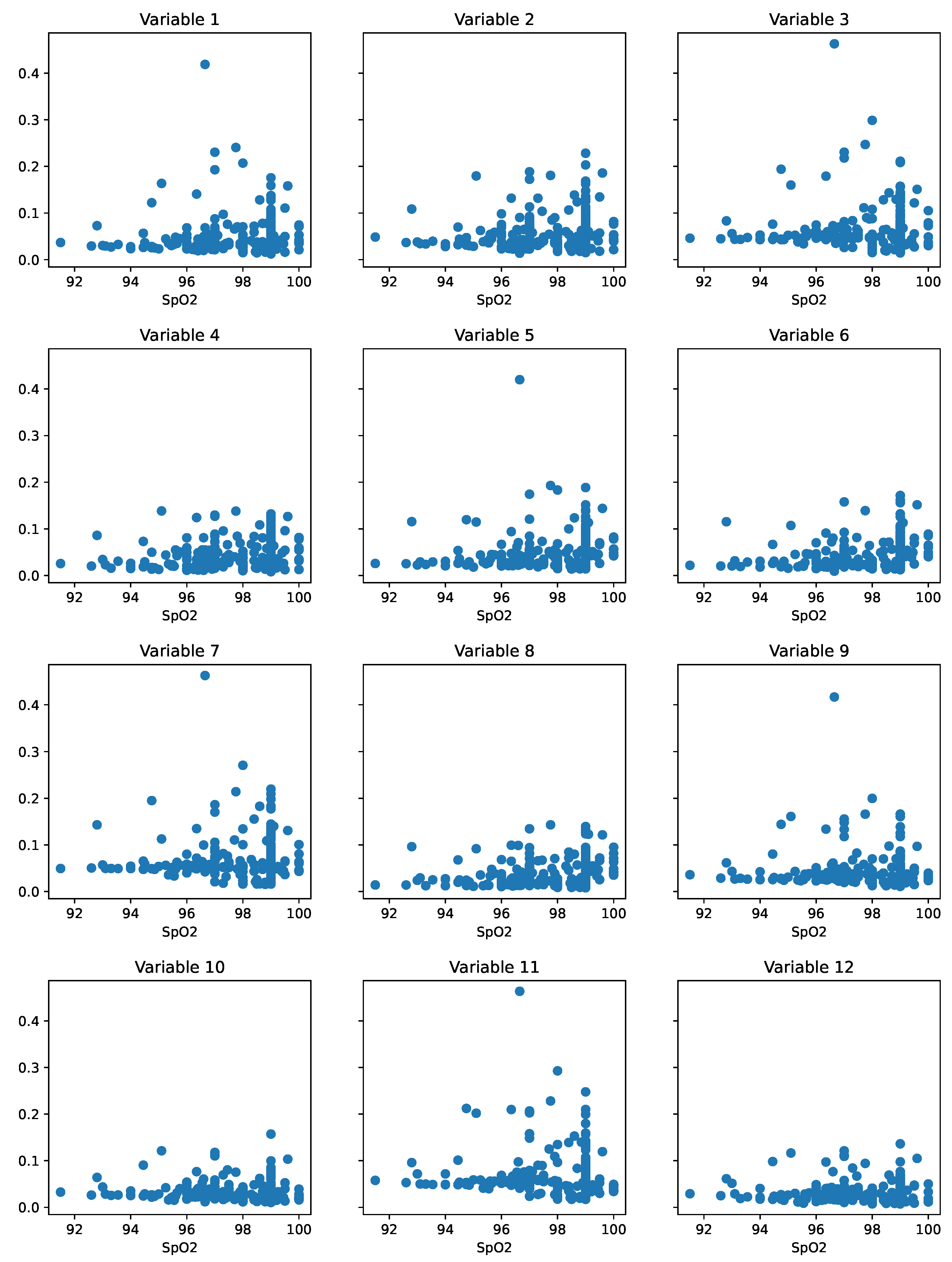
In previous studies, researchers have used the average of averages and the average of standard deviations from two colour channels of an RGB camera to extract relevant information [8,10,25]. However, since we only have access to an infrared camera, which captures only one colour channel, we needed to adapt our approach. Therefore, we decided to explore whether the average of averages, the average of standard deviations, the standard deviation of averages, and the standard deviation of standard deviation can provide us with useful information that can improve the accuracy of our method. Our rationale behind using these statistical measures is based on the assumption that these values can help us quantify the distribution of pixel intensities within the image. In Figure 5, scatter plots for each of the 12 extracted variables are presented. It is evident from the scatter plots that different combinations of variable values can result in the same SpO2 value. This observation indicates the presence of non-uniqueness in the relationship between the variables and the SpO2 value. The non-uniqueness can be attributed to the complex physiological and environmental factors that affect SpO2 estimation, such as skin color, lighting conditions, and motion artifacts. It is important to note that the non-uniqueness of variable combinations can affect the accuracy and robustness of the SpO2 estimation algorithm. The combination of these variables has shown to improve the regression of SpO2 in our experiments; however, it is hard to visualize these dependencies.
V 4 ( i 1 ) + 1 mean t { mean x , y { I i ( x , y , t ) }
V 4 ( i 1 ) + 2 mean t { std x , y { I i ( x , y , t ) }
V 4 ( i 1 ) + 3 std t { mean x , y { I i ( x , y , t ) }
V 4 ( i 1 ) + 4 std t { std x , y { I i ( x , y , t ) }
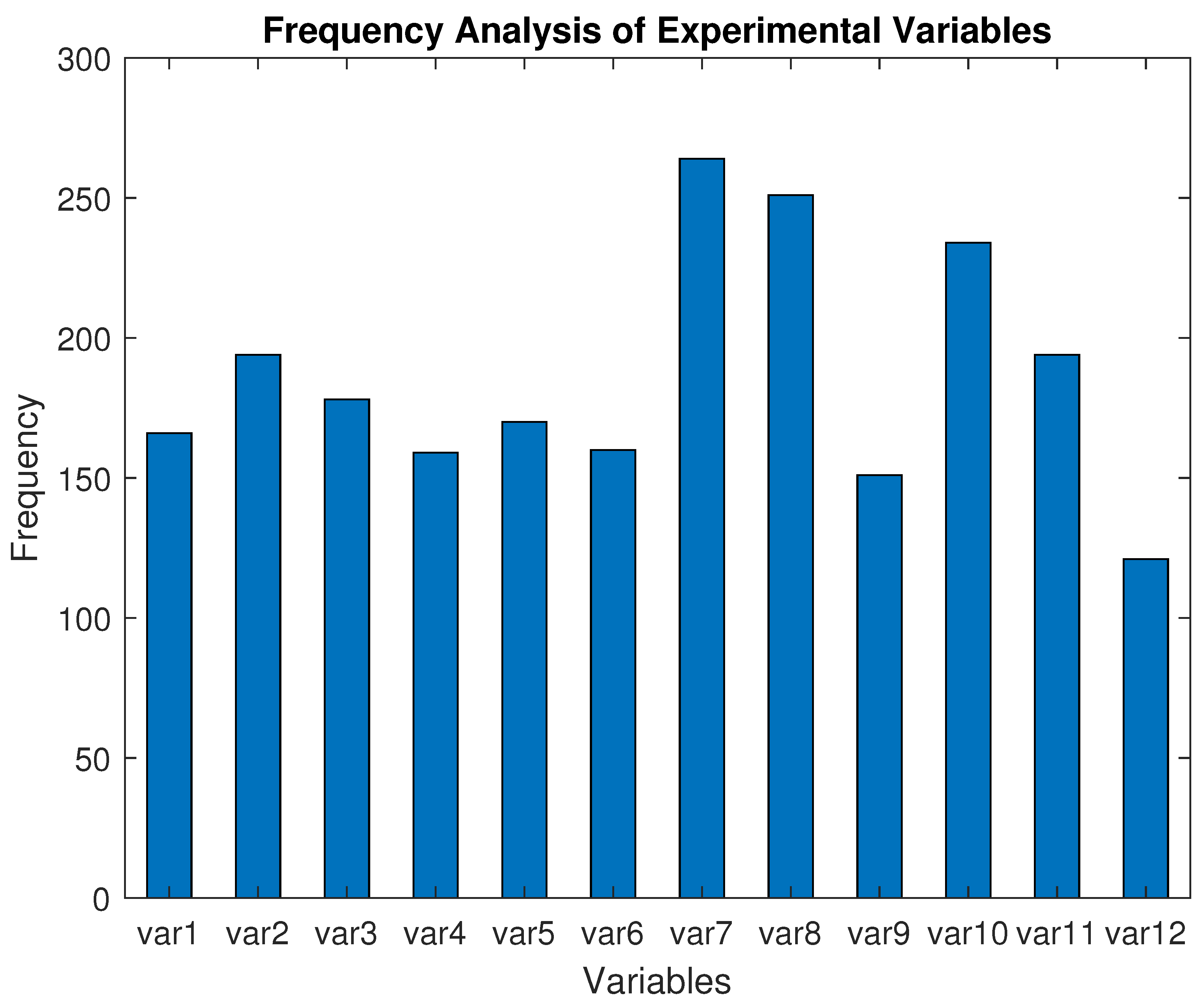
We adopt an approach in which we assign the extracted variables V j to the statistical characteristics of each frame sequence I i ( x , y , t ) as shown above, where i = 1 , 2 , 3 represents each of the three facial areas. This allows us to capture the variability in the variables within different facial regions and to identify which regions contribute the most to the overall SpO2 estimation. By constructing the collective histogram in Figure 6 containing the appearance frequency of each variable in the top-10 feature set from every machine learning algorithm, we are able to identify the most significant variables and their corresponding facial regions.

6.5. Parameters and Potential Biases

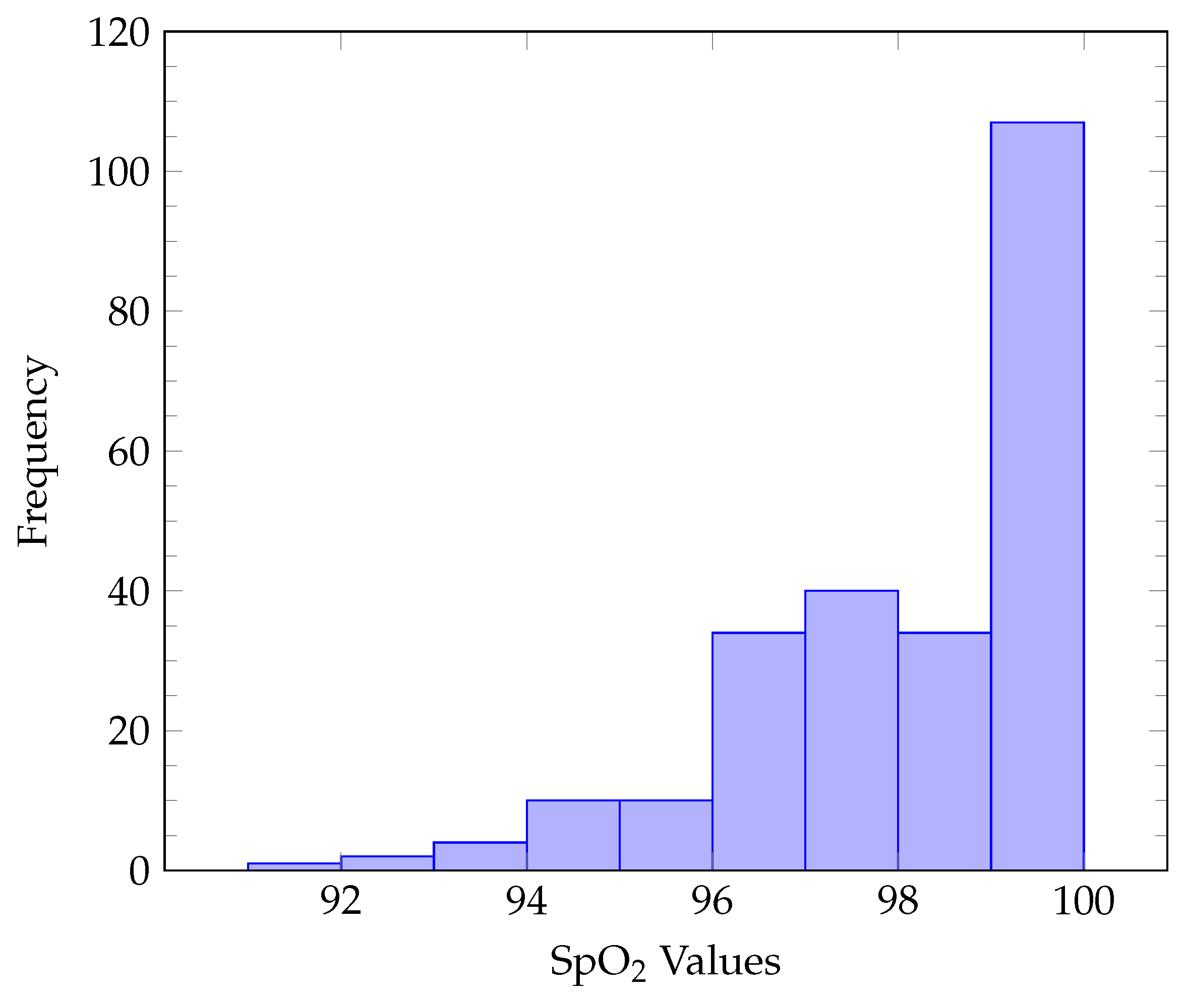
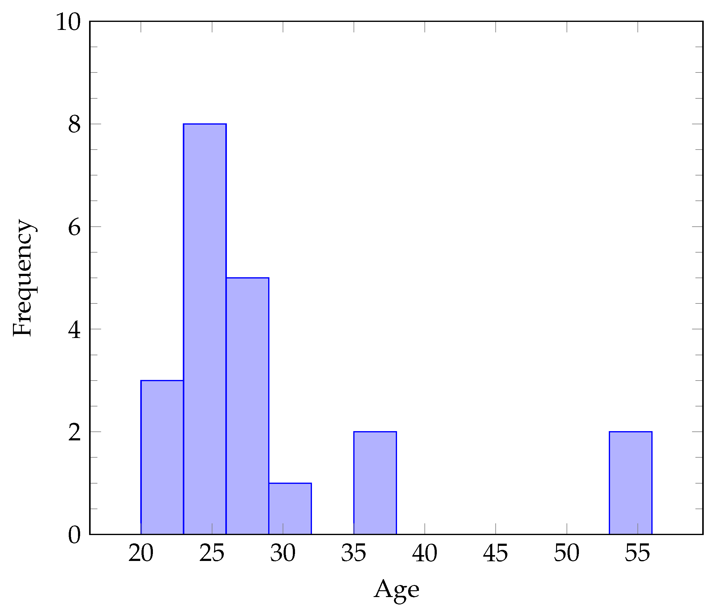
In Figure 7, we can see an histogram of the SpO2 measurement values in the collected dataset. In addition, Figure 8 contains the age distribution of all participants the dataset. It is evident from the histograms provided that the SpO2 measurement values are concentrated towards the higher end of the scale, with relatively fewer occurrences at the lower end of the spectrum. This shift to the right is a clear indication that the majority of the observations have higher SpO2 values, which may suggest a general trend towards better oxygen saturation levels among the studied population. It is not unexpected to observe a higher concentration of oxygen saturation readings towards the higher end of the scale for younger adults, as compared to older individuals. It is well documented in the medical literature that the baseline oxygen saturation levels of healthy individuals can vary based on their age, and that elderly individuals tend to have lower oxygen saturation readings compared to younger adults [42]. However, the underlying physiology of an individual is also an important factor that should be taken into consideration when evaluating a measurement reading. Various health conditions and lifestyle habits can affect the accuracy of pulse oximetry readings, which measure the oxygen saturation levels in the blood. For example, obesity, lung and cardiovascular diseases, emphysema, chronic obstructive pulmonary disease, congenital heart disease, and sleep apnea can lead to lower oxygen saturation levels [42]. Smoking can also impact the accuracy of pulse oximetry, especially if hypercapnia is present. Individuals with anemia may have normal oxygen saturation levels, but this may not indicate adequate oxygenation due to a lower amount of hemoglobin to carry oxygen [42]. For the previously stated reasons, it is essential to include individuals from a diverse demographic in any study or analysis of SpO2 measurements. This includes a representation of various age groups, both genders, individuals with a range of health statuses, smokers, and non-smokers. This helps to account for the different factors that can affect SpO2 readings. By including a representative sample of the population, the results of the study are more likely to be generalizable and relevant to a broader population. Furthermore, this helps to minimize any potential biases that may result from a limited sample, thereby increasing the reliability and validity of the results.

7. Conclusions

In this paper, we proposed a system to perform SpO2 estimation using an infrared commercial camera and facial videos. The proposed system uses infrared video for this task for the first time in order to enable contactless patient monitoring during night-time. The proposed approach uses motion magnification to enhance the facial video and extract three regions of interest, as well as twelve statistical features. A variety of machine and deep learning regression tools were used in a comparison study to infer the SpO2 value, most of which satisfy the FDA accuracy specifications. The Extra Trees Regressor appears to deliver the minimum RMSE, using only five out of the twelve extracted features. In the field of infrared photoplethysmography research, there has been limited prior work utilizing conventional affordable camera technology for the purpose of pulse oximetry. As a result, there are few direct comparisons that can be made to our approach. However, there are some past papers that have explored related topics using different methodologies and datasets. It is important to note that these prior works cover a range of techniques and may not directly reflect the strengths and limitations of our proposed method. Given the novelty of our approach and the limited prior work in this area, it is difficult to determine a clear state of the art. While it is uncertain whether infrared-based videos will outperform RGB-based videos in terms of accuracy, this should not be interpreted as a conflict between the two methods. Instead, it can be viewed as a means of obtaining a holistic view of SpO2 monitoring, as each approach may provide unique information that can complement and improve the overall accuracy of the system. Nevertheless, we aim to contribute to the field by providing a comprehensive and rigorous evaluation of our approach and its potential applications and by exploring the potential benefits of combining the outputs of both methods to further enhance the performance of SpO2 monitoring systems.

Author Contributions

Conceptualization, N.M., G.-A.C. and T.S.; methodology, T.S., G.-A.C. and N.M.; software, T.S.; validation, T.S. and G.-A.C.; formal analysis, N.M.; investigation, T.S.; writing—original draft preparation, T.S.; writing—review and editing, T.S., G.-A.C. and N.M.; supervision, N.M.; project administration, N.M.; funding acquisition, N.M. All authors have read and agreed to the published version of the manuscript.

Funding

This study was made possible through the project “Improvement of the Quality of Life and Activity for the Elderly” (MIS 5047294) which was implemented under the “Support for Regional Excellence” program, financed by the “Competitiveness, Entrepreneurship and Innovation” program (NSRF 2014-2020) and funded jointly by Greece and the European Union (European Regional Development Fund).

Institutional Review Board Statement

Ethical review and approval were waived for this study, due to the fact that the measurement of SpO2 is a simple non-invasive medical measurement performed by people at home without any special training.

Informed Consent Statement

Written informed consent has been obtained from all participants in the study, including the patient(s) whose information is included in this paper. The consent form includes a full explanation of the nature and purpose of the study, as well as any potential risks and benefits of participation. The participants were informed that their participation is voluntary, and that they have the right to withdraw from the study at any time without any negative consequences. The participants were also informed that their information will be kept confidential and anonymous, and that the data collected will only be used for the purposes of the research study.

Data Availability Statement

The developed code and data used in this study can be found at the mentioned link: https://github.com/TomStog/Infrared-SpO2 (accessed on 16 May 2023).

Acknowledgments

The researchers would like to extend their appreciation to all participants who volunteered for the study.

Conflicts of Interest

The authors declare that they have no financial, personal, or professional conflict of interest that may have influenced the design, conduct, analysis, or interpretation of this study. Additionally, the authors have not been involved in any other studies or research projects that could be perceived as conflicting with the current study. The authors assure that the results of this study have been reported honestly and accurately, and that the data presented has not been manipulated or falsified in any way.

References

  1. “Heart Health and Aging”. National Institute on Aging. U.S. Department of Health and Human Services. 1 June 2018. Available online: https://www.nia.nih.gov/health/heart-health-and-aging (accessed on 16 May 2023).
  2. Gooneratne, N.S.; Patel, N.P.; Corcoran, A. Chronic Obstructive Pulmonary Disease Diagnosis and Management in Older Adults. J. Am. Geriatr. Soc. 2010, 58, 1153–1162. [Google Scholar] [CrossRef]
  3. Semelka, M.; Wilson, J.; Floyd, R. Review of Diagnosis and Treatment of Obstructive Sleep Apnea in Adults. Am. Fam. Phy. 2016, 94, 355–360. [Google Scholar]
  4. “COPD-Symptoms|NHLBI, NIH”. National Heart Lung and Blood Institute. U.S. Department of Health and Human Services; 24 March 2022. Available online: https://www.nhlbi.nih.gov/health/copd/symptoms (accessed on 16 May 2023).
  5. Ling, I.T.; James, A.L.; Hillman, D.R. Interrelationships between Body Mass, Oxygen Desaturation, and Apnea-Hypopnea Indices in a Sleep Clinic Population. Sleep 2012, 35, 89–96. [Google Scholar] [CrossRef] [PubMed]
  6. Cui, J.; Mao, X.; Olman, V.; Hastings, P.J.; Xu, Y. Hypoxia and Miscoupling between Reduced Energy Efficiency and Signaling to Cell Proliferation Drive Cancer to Grow Increasingly Faster. J. Mol. Cell Biol. 2012, 4, 174–176. [Google Scholar] [CrossRef] [PubMed]
  7. O’Driscoll, B.R.; Howard, L.S.; Earis, J.; Mak, V. British Thoracic Society Guideline for Oxygen Use in Adults in Healthcare and Emergency Settings. BMJ Open Respir. Res. 2017, 4, e000170. [Google Scholar] [CrossRef] [PubMed]
  8. Kong, L.; Zhao, Y.; Dong, L.; Jian, Y.; Jin, X.; Li, B.; Feng, Y.; Liu, M.; Liu, X.; Wu, H. Non-Contact Detection of Oxygen Saturation Based on Visible Light Imaging Device Using Ambient Light. Opt. Express 2013, 21, 17464–17471. [Google Scholar] [CrossRef]
  9. Moço, A.; Verkruysse, W. Pulse Oximetry Based on Photoplethysmography Imaging with Red and Green Light. J. Clin. Monit. Comput. 2021, 35, 123–133. [Google Scholar] [CrossRef]
  10. De Fátima Galvão Rosa, A.; Betini, R.C. Noncontact SPO2 Measurement Using Eulerian Video Magnification. IEEE Trans. Instrum. Meas. 2019, 69, 2120–2130. [Google Scholar] [CrossRef]
  11. Verkruysse, W.; Bartula, M.; Bresch, E.; Rocque, M.; Meftah, M.; Kirenko, I. Calibration of Contactless Pulse Oximetry. Anesth. Analg. 2017, 124, 136–145. [Google Scholar] [CrossRef]
  12. Nemcova, A.; Jordanova, I.; Varecka, M.; Smisek, R.; Marsanova, L.; Smital, L.; Vitek, M. Monitoring of Heart Rate, Blood Oxygen Saturation, and Blood Pressure Using a Smartphone. Biomed. Signal Process. Control 2020, 59, 101928. [Google Scholar] [CrossRef]
  13. Rasche, S.; Huhle, R.; Junghans, E.; de Abreu, M.G.; Ling, Y.; Trumpp, A.; Zaunseder, S. Association of Remote Imaging Photoplethysmography and Cutaneous Perfusion in Volunteers. Sci. Rep. 2020, 10, 16464. [Google Scholar] [CrossRef]
  14. Rogers, J. An Introduction to Cardiovascular Physiology; Butterworth-Heinemann: Oxford, UK, 2009. [Google Scholar]
  15. Briers, D.; Duncan, D.D.; Hirst, E.; Kirkpatrick, S.J.; Larsson, M.; Steenbergen, W.; Stromberg, T.; Thompson, O.B. Laser Speckle Contrast Imaging: Theoretical and Practical Limitations. J. Biomed. Opt. 2013, 18, 066018. [Google Scholar] [CrossRef]
  16. Tamura, T. Current Progress of Photoplethysmography and SPO2 for Health Monitoring. Biomed. Eng. Lett. 2019, 9, 21–36. [Google Scholar] [CrossRef]
  17. Akamatsu, Y.; Onishi, Y.; Imaoka, H. Blood Oxygen Saturation Estimation from Facial Video via DC and AC components of Spatio-temporal Map. arXiv 2022, arXiv:2212.07116. [Google Scholar]
  18. Wu, H.Y.; Rubinstein, M.; Shih, E.; Guttag, J.; Durand, F.; Freeman, W. Eulerian Video Magnification for Revealing Subtle Changes in the World. ACM Trans. Graph. 2012, 31, 65. [Google Scholar] [CrossRef]
  19. Akamatsu, Y.; Onishi, Y.; Imaoka, H. Heart Rate and Oxygen Saturation Estimation from Facial Video with Multimodal Physiological Data Generation. In Proceedings of the ICASSP 2022—2022 IEEE International Conference on Acoustics, Speech and Signal Processing (ICASSP), Singapore, 23–27 May 2022. [Google Scholar]
  20. Viola, P.; Jones, M. Rapid Object Detection Using a Boosted Cascade of Simple Features. In Proceedings of the IEEE Computer Society Conference on Computer Vision and Pattern Recognition (CVPR), Kauai, HI, USA, 8–14 December 2001. [Google Scholar]
  21. Milutinovic, J.; Zelic, K.; Nedeljkovic, N. Evaluation of Facial Beauty Using Anthropometric Proportions. Sci. World J. 2014, 2014, 428250. [Google Scholar] [CrossRef]
  22. Kaya, K.S.; Türk, B.; Cankaya, M.; Seyhun, N.; Coşkun, B.U. Assessment of Facial Analysis Measurements by Golden Proportion. Braz. J. Otorhinolaryngol. 2019, 85, 494–501. [Google Scholar] [CrossRef]
  23. Fernandes, J.W. The Legacy of Art in Plastic Surgery. Plast. Reconstr. Surg. Glob. Open 2021, 9, e3519. [Google Scholar] [CrossRef]
  24. Garratt, C.; Ward, D.; Antoniou, A.; Camm, A.J. Misuse of Verapamil in Pre-Excited Atrial Fibrillation. Lancet 1989, 333, 367–369. [Google Scholar] [CrossRef]
  25. Brieva, J.; Moya-Albor, E.; Ponce, H. A Non-Contact SpO2 Estimation Using a Video Magnification Technique. In Proceedings of the 17th International Symposium on Medical Information Processing and Analysis, Campinas, Brazil, 17–19 November 2021. [Google Scholar]
  26. Lauridsen, H.; Hedwig, D.; Perrin, K.L.; Williams, C.J.; Wrege, P.H.; Bertelsen, M.F.; Pedersen, M.; Butcher, J.T. Extracting Physiological Information in Experimental Biology via Eulerian Video Magnification. BMC Biol. 2019, 17, 103. [Google Scholar] [CrossRef]
  27. Hastie, T.; Tibshirani, R. Generalized Additive Models. Stat. Sci. 1986, 1, 3. [Google Scholar] [CrossRef]
  28. MacCullagh, P.; Nelder, J.A. Generalized Linear Models; Chapman and Hall: London, UK, 1989. [Google Scholar]
  29. Servén, D.; Brummitt, C. “A Tour of PyGAM”. A Tour of pyGAM-pyGAM Documentation. 2018. Available online: https://pygam.readthedocs.io/en/latest/notebooks/tour_of_pygam.html (accessed on 16 May 2023).
  30. Geurts, P.; Ernst, D.; Wehenkel, L. Extremely Randomized Trees. Mach. Learn. 2006, 63, 3–42. [Google Scholar] [CrossRef]
  31. Kingma, D.P.; Ba, J. Adam: A Method for Stochastic Optimization. arXiv 2014, arXiv:141 2.6980. [Google Scholar]
  32. He, K.; Zhang, X.; Ren, S.; Sun, J. Delving Deep into Rectifiers: Surpassing Human-Level Performance on ImageNet Classification. In Proceedings of the IEEE International Conference on Computer Vision (ICCV), Santiago, Chile, 7–13 December 2015; pp. 1026–1034. [Google Scholar]
  33. Singh, S.P.; Wang, L.; Gupta, S.; Goli, H.; Padmanabhan, P.; Gulyás, B. 3D Deep Learning on Medical Images: A Review. Sensors 2020, 20, 5097. [Google Scholar] [CrossRef] [PubMed]
  34. Kim, S.Y.; Lim, J.; Na, T.; Kim, M. 3DSRnet: Video Super-resolution using 3D Convolutional Neural Networks. arXiv 2018, arXiv:1812.09079. [Google Scholar]
  35. Kim, D.E.; Gofman, M. Comparison of Shallow and Deep Neural Networks for Network Intrusion Detection. In Proceedings of the IEEE 8th Annual Computing and Communication Workshop and Conference (CCWC), Las Vegas, NV, USA, 8–10 January 2018. [Google Scholar]
  36. Song, Y.; Cai, Y.; Tan, L. Video-Audio Emotion Recognition Based on Feature Fusion Deep Learning Method. In Proceedings of the 2021 IEEE International Midwest Symposium on Circuits and Systems (MWSCAS), East Lansing, MI, USA, 9–11 August 2021. [Google Scholar]
  37. Arnab, A.; Dehghani, M.; Heigold, G.; Sun, C.; Lucic, M.; Schmid, C. Vivit: A Video Vision Transformer. In Proceedings of the IEEE/CVF International Conference on Computer Vision (ICCV), Montreal, BC, Canada, 11–17 October 2021. [Google Scholar]
  38. Dosovitskiy, A.; Beyer, L.; Kolesnikov, A.; Weissenborn, D.; Zhai, X.; Unterthiner, T.; Dehghani, M.; Minderer, M.; Heigold, G.; Gelly, S.; et al. An Image Is Worth 16 × 16 Words: Transformers for Image Recognition at Scale. arXiv 2020, arXiv:2010.11929. [Google Scholar]
  39. Gosthipaty, A.; Thakur, A. Keras Documentation: Video Vision Transformer. Video Vision Transformer. Keras. 12 January 2022. Available online: https://keras.io/examples/vision/vivit/ (accessed on 16 May 2023).
  40. ISO (International Organization for Standardization). ISO 80601-2-61: Medical Electrical Equipment—Part 2-61: Particular Requirements for the Basic Safety and Essential Performance of Diagnostic Ultrasound Equipment; ISO: Geneva, Switzerland, 2019. [Google Scholar]
  41. Pulse Oximeter Accuracy and Limitations. U.S. Food and Drug Administration. FDA; 7 November 2022. Available online: https://www.fda.gov/medical-devices/safety-communications/pulse-oximeter-accuracy-and-limitations-fda-safety-communication (accessed on 16 May 2023).
  42. Lapum, J.L.; Verkuyl, M.; Garcia, W.; St-Amant, O.; Tan, A. Vital Sign Measurement across the Lifespan—1st Canadian Edition; eCampusOntario: Toronto, ON, Canada, 2019. [Google Scholar]
Figure 1. A flowchart of the proposed SpO2 estimation methodology. In terms of regression, the flowchart mainly demonstrates that in our experiments, both traditional machine learning and deep learning regression algorithms were tested but not used simultaneously.
Information 14 00301 g001
Figure 2. The proportion analysis of the human face involves focusing on specific regions of interest, such as the forehead and the left/right cheek, which are highlighted.
Information 14 00301 g002
Figure 3. The experimental setup that was used during our experiment. The subject is seated at a fixed distance from the camera and instructed to stay still and look at the camera. The right arm of the subject is placed on the table and a commercial oximeter measures the real SpO2 values from the index finger of the right hand.
Information 14 00301 g003
Figure 4. (Above) A family of b-spline basis functions. (below) Penalized B-splines allow us to automatically model non-linear relationships [29].
Information 14 00301 g004
Figure 5. A collection of scatter plots for each of the 12 variables.
Information 14 00301 g005
Figure 6. Collective variables’ appearance frequency histogram.
Information 14 00301 g006
Figure 7. SpO2 Measurement distribution of the participants in the created dataset.
Information 14 00301 g007
Figure 8. Volunteer age distribution of the participants in the created dataset.
Information 14 00301 g008
Table 1. A collective performance overview of the algorithms used. RMSE and absolute error scores are expressed in percentage terms (best performance in bold).
Regression AlgorithmAverage RMSEMinimum RMSEMAEMAPE R 2 ScoreNo. Features
Linear Regression1.5651.4811.2060.0120.1555
Ridge1.5991.5821.3040.0130.02411
SGD Regressor1.9191.8631.6510.017−0.4243
ElasticNet1.6151.6121.3180.014−0.0095
Lars1.5741.4831.2130.0130.1264
Lasso (alpha = 10 4 )1.6121.6041.3160.0140.0007
LassoLars (alpha = 10 4 )1.5651.5231.2600.0140.0007
Huber Regressor1.5811.4981.1790.0120.1496
Quantile Regressor1.7531.7301.2720.013−0.1583
RANSAC Regressor1.8801.8401.2790.013−0.1985
Theilsen Regressor1.6741.5121.2680.0130.1064
Poisson Regressor1.6151.6121.3180.0140.0006
Tweedie Regressor1.6151.6121.3180.0140.0008
Gamma Regressor1.6151.6121.3180.0140.00011
AdaBoost Regressor (5, 50, 0.1) 11.3521.2350.9560.0100.3865
AdaBoost Regressor (5, 100, 0.1) 11.3431.2260.9570.0100.4115
AdaBoost Regressor (10, 50, 0.1) 11.4101.2450.9270.0100.4287
AdaBoost Regressor (10, 100, 0.1) 11.4011.2460.9230.0100.3986
Bagging Regressor (5, 50) 21.3551.2300.9800.0100.3745
Bagging Regressor (10, 50) 21.3911.1890.9270.0100.4278
Bagging Regressor (5, 100) 21.3461.2120.9750.0100.3939
Bagging Regressor (10, 100) 21.3791.2020.9200.0100.4066
Extra Trees Regressor (50) 31.3371.1840.9640.0100.4656
Extra Trees Regressor (100) 31.3311.1710.9600.0100.4655
HistGradientBoosting Regressor1.3861.2341.0190.0110.4105
Gradient Boosting Regressor (100, 0.01, 3) 41.4121.3391.0970.0110.3156
Gradient Boosting Regressor (100, 0.01, 5) 41.4011.2771.0630.0110.37510
Gradient Boosting Regressor (100, 0.1, 3) 41.4241.2431.0380.0110.3788
Gradient Boosting Regressor (100, 0.1, 5) 41.4441.2561.0330.0110.3728
Gradient Boosting Regressor (500, 0.01, 3) 41.3911.2581.0230.0110.3935
Gradient Boosting Regressor (500, 0.01, 5) 41.4221.2481.0190.0100.3837
Gradient Boosting Regressor (500, 0.1, 3) 41.4691.2721.0730.0110.3628
Gradient Boosting Regressor (500, 0.1, 5) 41.4481.2651.0370.0110.39510
Random Forest Regressor (100, 3) 51.3801.2921.0440.0110.3458
Random Forest Regressor (100, 5) 51.3551.2540.9970.0100.4124
OxygeNN1.7111.5321.3560.0140.0066
Generalized Additive Model (4 splines)1.5731.5261.1700.012−0.00812
Generalized Additive Model (6 splines)1.4641.4131.0710.0110.12012
Generalized Additive Model (8 splines)1.5131.4071.0920.0110.06112
Generalized Additive Model (10 splines)1.5341.3831.0930.0110.11812
Generalized Additive Model (12 splines)1.4911.4351.0850.0110.04312
Generalized Additive Model (14 splines)1.4911.4271.0790.0110.11812
3D-CNN (single-source model)1.5921.5701.2960.0130.000-
3D-CNN (multi-source model)1.5941.5641.2980.013−0.002-
ViViT1.6851.6151.3300.013−0.040-
1 (max depth, estimators, learning rate) 2 (max depth, estimators) 3 (estimators) 4 (estimators, learning rate, max depth) 5 (estimators, max depth).
Table 2. The Proposed ANN architecture called “OxygeNN”.
Layer/StrideContentsOutput Size
Input Features 12 × 1 -
FC1 D e n s e ( 128 ) A c t i v a t i o n = R e L U D r o p o u t ( p = 0.2 ) i n i t i a l i z e r = h e _ u n i f o r m 128
FC2 D e n s e ( 256 ) A c t i v a t i o n = R e L U D r o p o u t ( p = 0.2 ) i n i t i a l i z e r = h e _ u n i f o r m 256
FC3 D e n s e ( 128 ) A c t i v a t i o n = R e L U D r o p o u t ( p = 0.2 ) i n i t i a l i z e r = h e _ u n i f o r m 128
FC4 D e n s e ( 64 ) A c t i v a t i o n = R e L U i n i t i a l i z e r = h e _ u n i f o r m 64
Output D e n s e ( 1 ) A c t i v a t i o n = L i n e a r 1
Table 3. The proposed single-source 3D-CNN architecture for video sequences.
Layer/StrideContentsOutput Size (H × W × D × C)
Input Clip-64 × 128 × 300 × 1
Conv3D C o n v 3 D ( 16 , k e r n e l = ( 5 , 5 , 5 ) ) M a x P o o l i n g 3 D ( p o o l = ( 3 , 3 , 3 ) ) D r o p o u t ( p = 0.5 ) A c t i v a t i o n = R e L U i n i t i a l i z e r = h e _ u n i f o r m 20 × 41 × 98 × 16
Conv3D C o n v 3 D ( 32 , k e r n e l = ( 5 , 5 , 5 ) ) M a x P o o l i n g 3 D ( p o o l = ( 3 , 3 , 3 ) ) D r o p o u t ( p = 0.5 ) A c t i v a t i o n = R e L U i n i t i a l i z e r = h e _ u n i f o r m 5 × 12 × 31 × 32
Flatten-59,520
FC1 D e n s e ( 128 ) A c t i v a t i o n = R e L U i n i t i a l i z e r = h e _ u n i f o r m 128
FC2 D e n s e ( 128 ) A c t i v a t i o n = R e L U i n i t i a l i z e r = h e _ u n i f o r m 128
Output D e n s e ( 1 ) A c t i v a t i o n = L i n e a r 1
Disclaimer/Publisher’s Note: The statements, opinions and data contained in all publications are solely those of the individual author(s) and contributor(s) and not of MDPI and/or the editor(s). MDPI and/or the editor(s) disclaim responsibility for any injury to people or property resulting from any ideas, methods, instructions or products referred to in the content.