Article

Quadrilateral Mesh Generation Method Based on Convolutional Neural Network

School of Computer Science and Technology, Hangzhou Dianzi University, Hangzhou 310018, China
*
Author to whom correspondence should be addressed.
Information 2023, 14(5), 273; https://doi.org/10.3390/info14050273
Submission received: 30 March 2023 / Revised: 28 April 2023 / Accepted: 1 May 2023 / Published: 4 May 2023

Abstract

:
The frame field distributed inside the model region characterizes the singular structure features inside the model. These singular structures can be used to decompose the model region into multiple quadrilateral structures, thereby generating a block-structured quadrilateral mesh. For the generation of block-structured quadrilateral mesh for two-dimensional geometric models, a convolutional neural network model is proposed to identify the singular structure inside the model contained in the frame field. By training the network model with a large number of model region decomposition data obtained in advance, the model can identify the vectors of the frame field in the region located in the segmentation field. Then, the segmentation streamline is constructed from the annotation. Based on this, the geometric region is decomposed into several small regions, regions which are then discretized with quadrilateral mesh elements. Finally, through two geometric models, it is verified that the convolutional neural network model proposed in this study can effectively identify the singular structure inside the model to realize the model region decomposition and block-structured mesh generation.

1. Introduction

Mesh generation is a preprocessing process in numerical simulation techniques, such as the finite element method, the finite volume method, and the finite difference method. This process decomposes a continuous geometric model into a combination of finite basic elements, which are called mesh elements [1,2]. According to the topological connection of mesh elements, meshes can be divided into structured meshes and unstructured meshes. Compared with unstructured meshes, structured meshes have the characteristics of high solution accuracy and fewer required elements [1]. However, due to the strong topological constraints of structured meshes, generating high-quality structured meshes for complex geometric models is nontrivial; it often requires a lot of manual work and high expertise from users [3,4,5,6,7,8,9]. An alternative way is to decompose the domain covered by the geometric model into several four-sided sub-domains and then generate structured meshes in each sub-domain. As a result, a block-structured mesh can be obtained. Additionally, the difficulty of structured mesh generation can be reduced to a certain extent [10].
However, for complex geometric models, the automation of domain decomposition is not an easy task; it needs to analyze the geometric characteristics of the models. In recent years, researchers have proposed methods to obtain the internal characteristics of the geometric model from the perspective of the physical field and found that the domain decomposition of the geometric model can be achieved by analyzing the singular structure of the physical field [7,8,9,10]. For example, Kowalski et al. [8] generated a smooth frame field inside the two-dimensional geometric model according to the principle of heat diffusion and finally obtained the decomposition of the model based on extracting the singular structures of the frame field. Xiao et al. [10] proposed to use the boundary element method to solve a vector Laplacian equation to obtain a smooth vector field inside the model and then obtain a smooth frame field reflecting the geometric characteristics of the boundary and finally achieve the decomposition of the model. In this type of method, the constructed smooth frame field takes into account the characteristics of both the boundary and the internal structure of the model. Therefore, the domain decomposition results can ensure block-structured meshes with high quality. In addition, the mesh elements near boundaries have good orthogonality as a result of the consideration of boundary characteristics in the generation of the frame field.
The domain decomposition method based on the singular structure analysis of the frame field greatly improves the automation of the process of generating high-quality block-structured meshes for complex geometries. The two key steps in such kind of methods are constructing a smooth frame field covering the geometric domain and extracting streamlines that decompose the domain according to the singular structures of the frame field. There are many ways to obtain a smooth frame field in the first step [7,8,9,10]. However, the second step relies on numerical methods to generate streamlines on discrete mesh elements. Normally, after the generation of initial streamlines, complex operations, such as streamline simplification and merging, are often required [10], and the algorithm still has robustness issues due to the adoption of the numerical method. In addition, for a local modification of the geometric model that often occurs in the engineering design, in order to obtain the block-structured mesh of the modified model, it is often necessary to regenerate a new frame field and re-extract the streamlines based on the new frame field. Undoubtedly, this increases the complexity of the mesh generation task. It is worth noting that when the topology of the geometric model does not change, the singular structure of the frame field inside the geometric model will not change, so the topology of the final model domain decomposition remains consistent. Aiming at this problem, this study presents an intelligent method for the identification of singular structures of a frame field based on a convolutional neural network, which realizes the identification of internal features of the geometric model and automatic domain decomposition, and finally realizes the block-structured mesh generation of the internal region of the geometric model.
Artificial intelligence methods have achieved great success in engineering applications, among which deep-learning methods are particularly popular [11,12]. For example, deep learning has been successfully used to compute offloading in the applications of the Internet of Things [13,14] and understand documents by analyzing page objects [15]. As a type of method in deep learning, convolutional neural networks are widely used in image and model processing [16,17,18,19]. A lot of work has also emerged in the feature recognition of geometric models. Qi et al. [20] pioneered a convolutional neural network model named PointNet in 2017, which directly acts on the point cloud model and uses the permutation invariance of points to learn the distribution characteristics of the point cloud of models. Additionally, in the PointNet++ [21] proposed in the same year, the sampling layer and grouping layer are adopted to enhance the ability to detect local features. Feng et al. [22] proposed the MeshNet, which uses mesh information as the input of the convolutional neural network. Wang et al. [23] proposed a convolutional neural network called dynamic graph convolutional neural network (DGCNN), which constructs a local neighborhood graph with k-nearest neighbors and performs convolution operations on the edges connecting neighboring pairs of points. It is reported that the DGCNN strengthens the extraction of local features of the point cloud model and improves the recognition ability. The artificial neural network has also been applied to the mesh generation area. As early as 2005, Yao et al. [24] proposed to use a neural network to learn the mesh generation characteristics of the two-dimensional advancing front method based on conditional judgment. The network can predict the position of the next front point and base on which a quadrilateral mesh element is generated. Recently, Wang et al. [25,26] proposed an advancing front triangular generation method and a mesh size control method based on neural networks; the effectiveness of the algorithm has been demonstrated with several geometric models.
The success of artificial intelligence methods in the processing of geometric models, such as point clouds, has shed light on the problem of domain decomposition. The frame field distributed inside the domain of a geometric model can be regarded as point cloud data. It includes both boundary features and internal features of the model, which can be used as the input data of a convolutional neural network. Inspired by this, a convolutional neural network is proposed to identify the internal singular structure of a model by analyzing the frame field inside the domain of this model. The neural network is trained through a large number of domain decomposition data, which can make the neural network identify the singular structure of the frame field. The trained neural network is then used to identify the vectors of frame components near the streamlines, and based on that, the streamlines are constructed to decompose the domain for block-structured mesh generation.

2. Model Data for Domain Decomposition

2.1. Domain Decomposition Based on the Frame Field

In Ref. [10], Xiao et al. proposed a block-structured quadrilateral mesh generation method based on the frame field. For completeness, the basics of the method are reviewed in this section.
The main idea is to generate a smooth frame field covering the model domain and then analyze the singularity in the frame field structure and generate the streamlines that partition the domain into four-sided sub-domains. Figure 1 shows the main steps of domain decomposition of a semicircle model based on the method proposed in Ref. [10]. The method takes a background mesh as an input (see Figure 1a), and a frame field is then computed on the background mesh nodes, as shown in Figure 1b. The frame field is computed by propagating the frames defined on the boundaries of the domain with a PDE-based method. In order to make the final quad elements align with the boundaries of the domain, the initial frames on the boundaries are set to be aligned with the boundaries (see Figure 1b). After the frame field is obtained in the geometric domain, the positions of the singularities of the field are determined, which are shown as the points in red in Figure 1c. Then, the streamlines emanating from these singularities are constructed, and these streamlines partition the domain into several four-sided sub-domains (see Figure 1d), which can be discretized with structured quadrilateral meshes.
The singular points and the streamlines partitioning the domain are called the singular structure of the frame field, and this provides a theoretical basis for the domain decomposition of the geometric model. Inspired by the above idea of domain decomposition, a convolutional neural network is proposed and trained to identify the singular structures of the frame field, and then, the singular structures are used for the domain decomposition of the model.

2.2. Training Data

As mentioned earlier in the Introduction section, local modifications of the geometric model often occur in the engineering design. For such applications, the topology structure of the geometries may not change, and thus, the singular structure of the frame field inside the geometric model will not change. The network in this study is trained to identify the singular structures for such geometries. Therefore, the training data for the network are only from the geometries with the same topology structure.
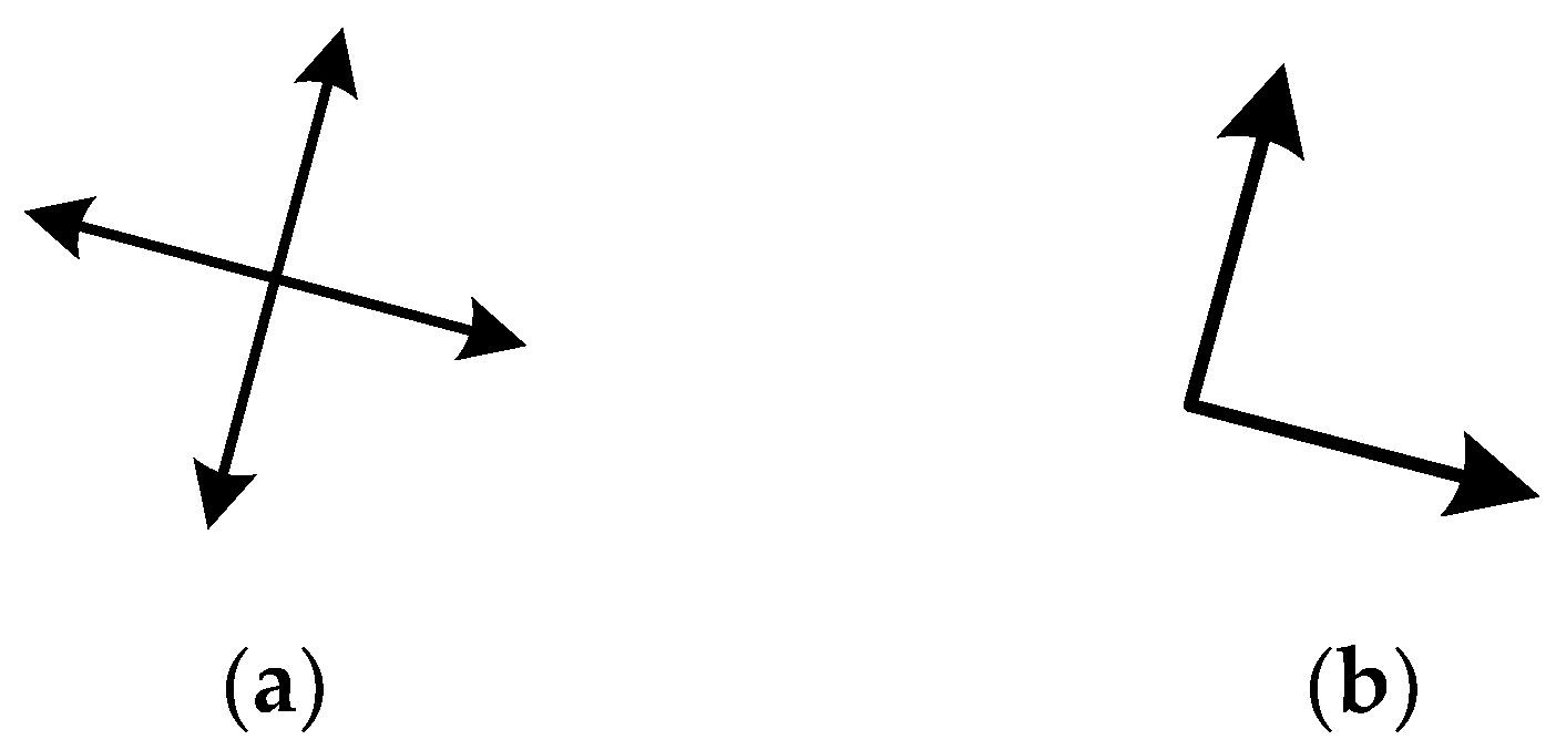
Overall, the background mesh nodes of each model are taken as the input point cloud data. Except for the coordinates information, a frame is attached to each node, and therefore, a discretized frame field is obtained over the point cloud. We expect the neural network to classify the frames on the background mesh nodes according to whether they lie on the streamlines that partition the model. Each two-dimensional frame is composed of four vector components (see Figure 2a). Considering the central symmetry of the frame vectors and the usage of the frame vectors in the generation of streamlines, each frame is represented by two independent vectors perpendicular to each other (see Figure 2b). Therefore, for each mesh node, we obtain two samples:
( x , y , v 1 , x , v 1 , y , l 1 ) ( x , y , v 2 , x , v 2 , y , l 2 )
where (x,y) are the coordinates of mesh nodes,  ( v i , x , v i , y )   ( i = 1 , 2 ) are the vector components of a frame on the mesh node, l i   ( i = 1 , 2 ) are the labels of the vector components (the value is 0 or 1).
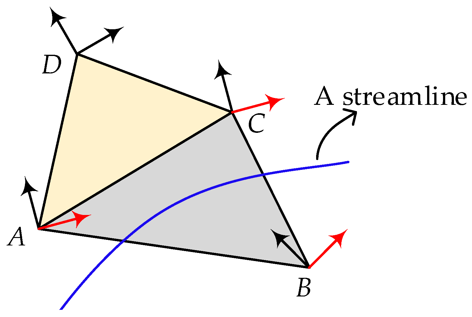
For the test data,  l i is predicted by the neural network, and based on that, streamlines are generated accordingly to partition the model domain. However, for the training data, the value of l i needs to be set in advance. Its value depends on the position of the mesh node and the angle between the vector component ( v i , x , v i , y ) and the streamline. The setting of l i is shown in Figure 3 according to the following rules: for the frame vectors on the nodes of a mesh element that a streamline goes through, the vectors that are consistent with the direction of the streamline are marked as 1 (see the arrows in red in Figure 3), and the vectors that are inconsistent with the direction of the streamline edge are marked as 0; for the frame vectors on the nodes of a mesh element that the streamlines do not go through, all are marked as 0 (see the vectors on node D in Figure 3). Figure 4 shows the frame components identified for the partition results shown in Figure 1. For the semicircle model shown in Figure 1, Figure 4a shows the background mesh and streamlines, and Figure 4b shows the vector components of frames marked near the streamlines according to the above rules, which are the vector components marked with label 1.
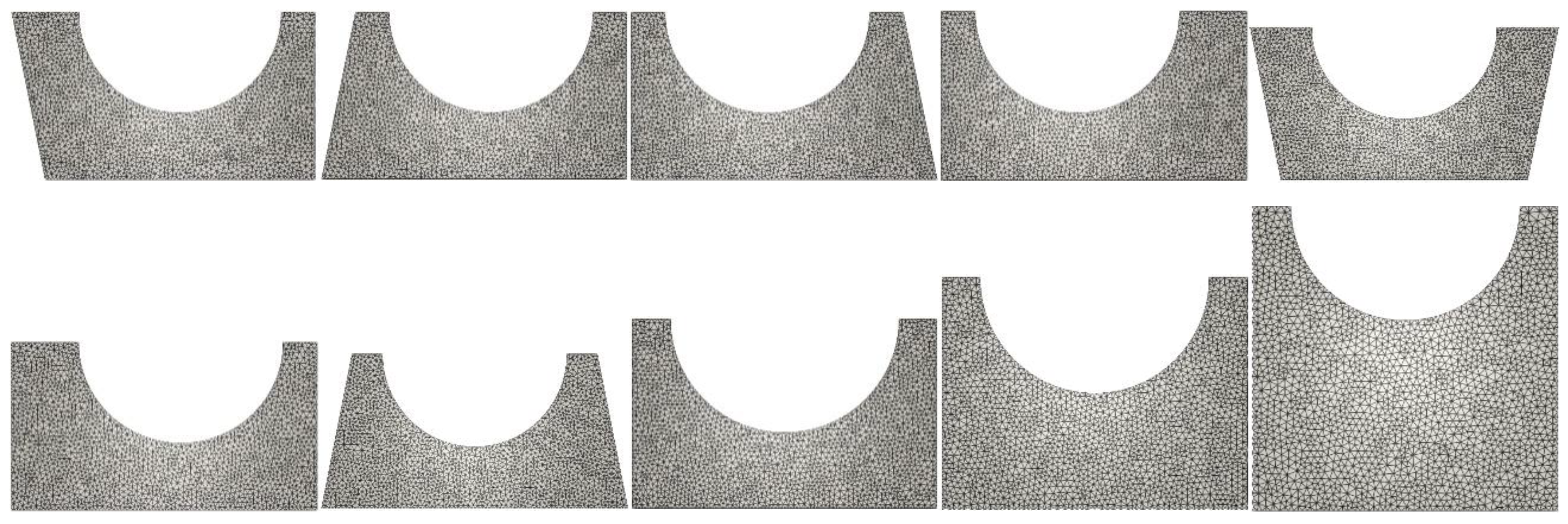
At this point, the training data for the neural network can be created. First, each two-dimensional geometric model is discretized with a triangular mesh with about 2048 nodes. Secondly, the method in Ref. [10] is used to generate a discretized frame field distributed on the mesh nodes and also the streamlines that partition the domain computed based on the frame field. Then, for each frame on a mesh node, select two mutually perpendicular vectors and set l i according to the rules mentioned above. In order to obtain a large number of training data, for each geometric model, more different test sample data sets are obtained through means such as rotation, deformation, and random movement of mesh points. Figure 5 shows part of the training data for the concave model.

3. Neural Network Model and Its Training

3.1. Neural Network Model

In order to classify the frame components near the streamlines, it is necessary to consider not only the local features but also the global features of the model. In this study, the EdgeConv operation proposed in Ref. [23] is used to extract the local features of the frame field, while the conventional convolution operation is used to extract the global features of the frame field.
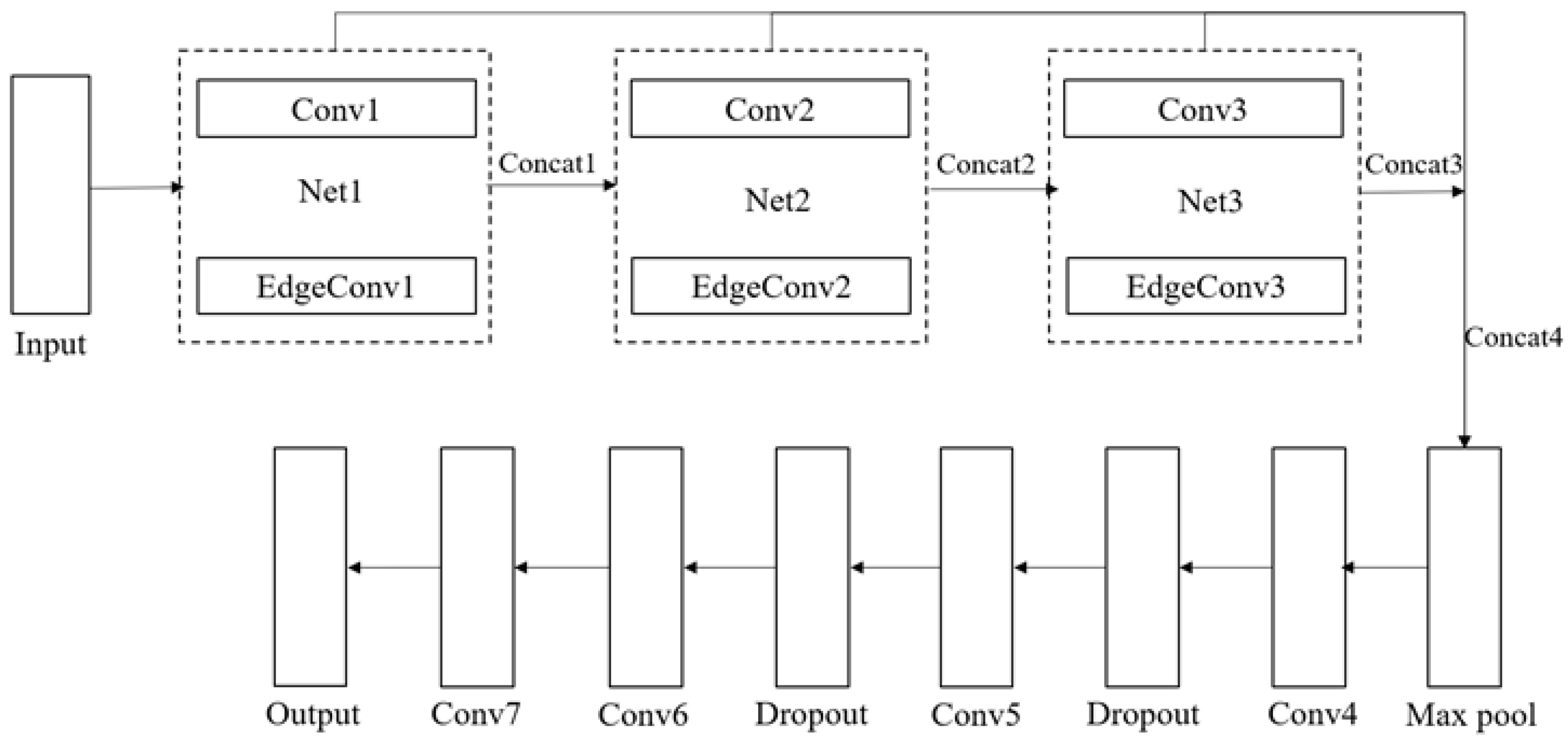
In this study, the TensorFlow platform is selected as the neural network development library. Figure 6 shows the convolutional neural network structure used to identify the singular structure of the frame field. The dimension of the input layer of the network is (N × 4), N is set to be the number of mesh nodes of each model (i.e., 2048), and 4 represents the data dimension on each mesh node (including the coordinates of the mesh node and frame component information). Subsequently, three feature extraction layers (Net1, Net2, and Net3) are added to enhance the ability of the network to capture features of the frame field. Each feature extraction layer includes edge convolution operations and regular convolution operations. The results of these two kinds of convolution operations are concatenated and used as the input of the next layer. The convolution kernel sizes in these three feature extraction layers are all (1 × 1), and the number of convolution channels is 16, 32, and 64, respectively. After Net3, the results of Net1, Net2, and Net3 are further concatenated and taken as the input of a maximum pooling layer (max pooling). Afterward, four more convolution layers with convolution kernel size (1 × 1) are introduced, and the number of convolution channels is 256, 256, 128, and 2, respectively. To avoid overfitting, a dropout layer is added after the first two convolutional layers, and the threshold is set to 0.5. In all convolutional layers, the padding is all set to be “VALID”. Finally, the output of the network is a two-category classification of semantic labels, identifying whether the frame component is located near the streamline and in the same direction as the streamline. Table 1 shows the more detailed parameter settings of the entire convolutional neural network structure.

3.2. Loss Function and Training

The domain decomposition problem in this study can be classified as a segmentation problem. The segmentation problem usually uses intersection over union (IoU) [23] as the evaluation standard, and the dice coefficient [27] is a key parameter when determining the IoU value. Considering the improvement of the IoU value and reducing the difficulty of neural network training convergence, the cross-entropy loss function and the dice loss function [27] are used as the loss function of the neural network training in this study, as follows:
l o s s = 0.5 l o s s 0 + 0.5 l o s s 1 ,
where l o s s 0 and l o s s 1 , are the cross-entropy loss function and the dice loss function, respectively, and the expressions are
l o s s 0 = | l a b e l s log ( z ) + ( 1 l a b e l s ) log ( 1 z ) | ,
l o s s 1 = 1 2 ( s u m ( z l a b e l s ) + 1 0 5 s u m ( z z ) + s u m ( l a b e l s l a b e l s ) + 1 0 5
where labels are the label vectors of the sample data set, and z is the result of the output layer configured with the Sigmoid activation function.
During training, the optimization algorithm we use is the stochastic gradient descent (SGD) method, the initial learning rate is 0.001, the momentum is 0.9, and the batch size is set to 4. The randomly selected 80% of the data from the sample data set is taken as the training data set, and the remaining 20% is taken as the test data set. After the training converges, IoU and overall accuracy (OA) are used to evaluate the experimental results.

4. Streamline Extraction and Quad Mesh Generation

Figure 7 presents the workflow of the proposed method. As can be seen, after the above convolutional neural network is trained, it can be used to predict the singular structure of a geometric model with the same topology. The prediction results identify the frame components that fall near the streamlines, which reflect the roughly singular structure of the geometric model. Based on this, the streamlines that partition the domain can be extracted, and finally, block-structured quad mesh can be generated.
Based on the prediction results of the neural network, the way to obtain streamlines is much simpler than the method in Ref. [10]. It is only necessary to find out the discrete line segments connected end to end in the prediction results. According to the existing frame field, the information related to singular points can be calculated according to the method in Ref. [10], such as the positions, the valences of the singular points, and the extension directions of the streamlines at a singular point. Suppose there are n singular points, denoted as s i (i = 1,…, n), and the corresponding extension directions of streamlines are v i , k (i = 1,…, n; k = 1,…, 3 or 1,…, 5), we extract all streamlines starting from the extension directions of the singularity. Taking the extension direction v i , k of the singular point s i as an example, the process of extracting the streamline l i , k is as follows:
(1)
Take the singular point s i and its extension direction v i , k as the initial current node (denoted as s c ) and the initial current extension direction (denoted as v c ), and add s c into the streamline l i , k , s c becoming a node of the streamline l i , k ;
(2)
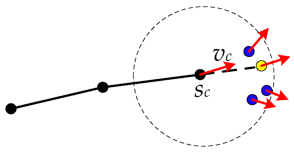
Among the nodes with frame components marked with label 1, find m neighboring nodes of the current node s c , denoted as n e i g i ( i = 1 , , m ) , and their frame components, denoted as v n e i g i ( i = 1 , , m ) . Let a n e i g c ( 1 c m ) be the closest node to s c , whose corresponding v n e i g c has the smallest angle with vector v c (then, n e i g c is regarded as the next node of the streamline), and add it into l i , k . Figure 8 presents the schematic for choosing the next node of the streamline; the nodes in blue in the circle centered at the current node s c are candidate neighboring nodes, and the node in yellow is the node that satisfies the above conditions, and therefore, it is chosen as the next node of the streamline;
(3)
Update the value of s c to be n e i g c , and the value of v c to be v n e i g c ;
(4)
If s c is a singular node or a boundary node, the entire streamline l i , k is extracted; otherwise, go to step 2.
In order to speed up the searching process of neighboring nodes, the approximate nearest neighbor (ANN) search algorithm is used in this study. Additionally, all the nodes predicted to be near the streamlines are organized with a binary search tree, such that the time complexity of searching for neighboring nodes of a node should be within O(logn) [28]. It should be noted that the streamlines obtained with the above method are formed by connecting discrete nodes, which may result in non-smooth streamlines. Therefore, after obtaining the initial streamlines, the Laplace smoothing method is used to smooth the streamlines. In addition, to obtain continuous streamlines, the continuous parameter expression of streamlines can be obtained with the curve fitting algorithm after the smoothing operation. For the predicted results shown in Figure 4b, the green line in Figure 9a shows the streamlines of the semicircle model obtained after the above process; they are used to partition the domain.
After all the streamlines are obtained, the model domain is partitioned into multiple sub-domains, and each sub-domain can be transformed into a four-sided domain. Therefore, the mapping method can be used to generate high-quality quadrilateral meshes for each sub-domain. In order to make the mesh conform to the shared edges of neighboring sub-domains, it is usually necessary to solve a linear programing problem to compute the number of discrete segments on each edge before mesh generation [10]. Figure 9b shows the final block-structured quadrilateral mesh of the semicircle model.

5. Results

In order to verify the effectiveness of the proposed algorithm, two different topologies are selected as examples for testing, and they are the concave topology and the four-hole topology. The convolutional neural network proposed in Section 3.1 is trained first with the training data. Note that a small part of the mesh data are obtained with in-house mesh generation code, and the remaining data are obtained with the data augmentation techniques mentioned in Section 2.2. Then, the frame field on a new mesh model is used for prediction with the trained neural network, based on which the geometric model is partitioned.
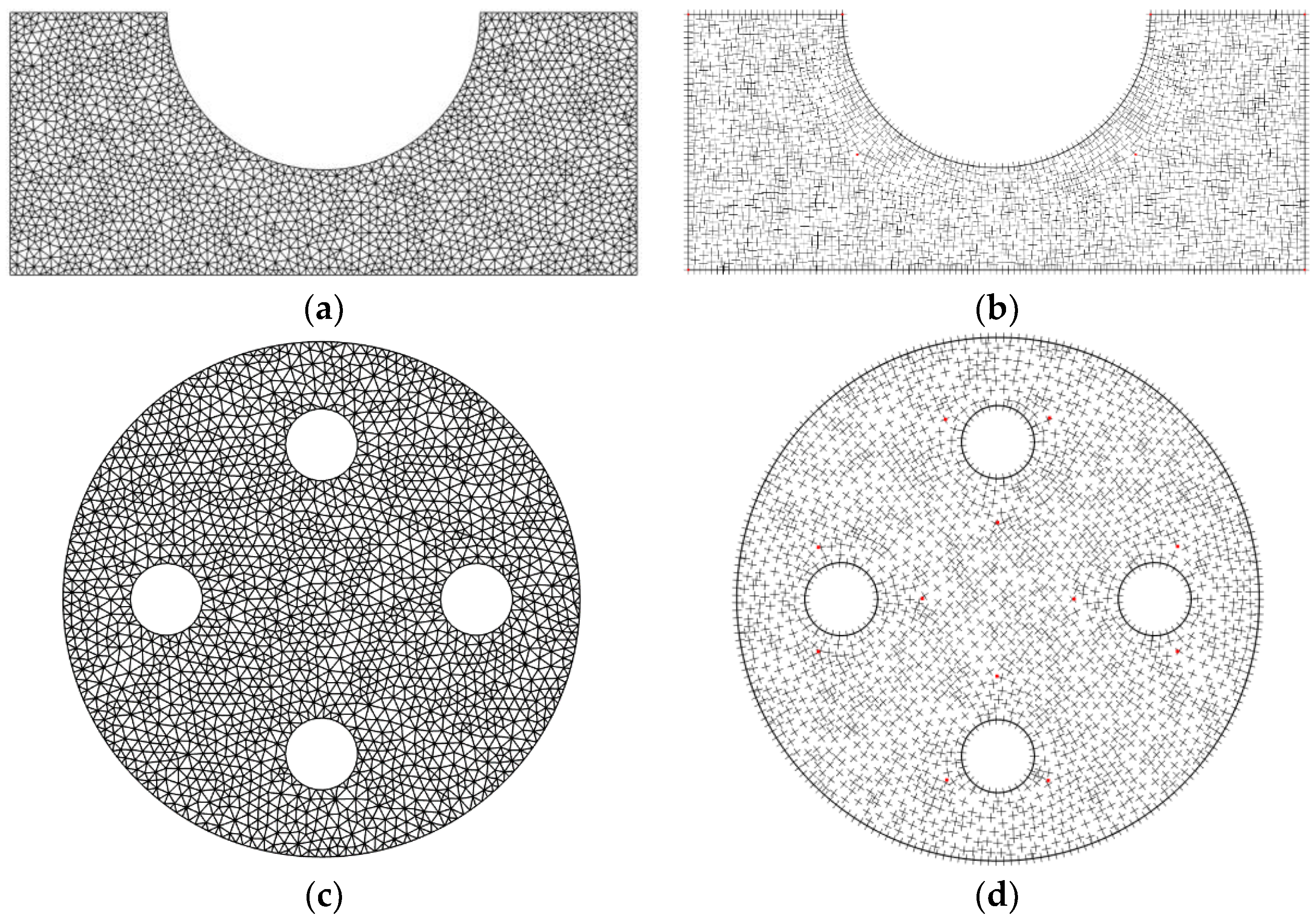
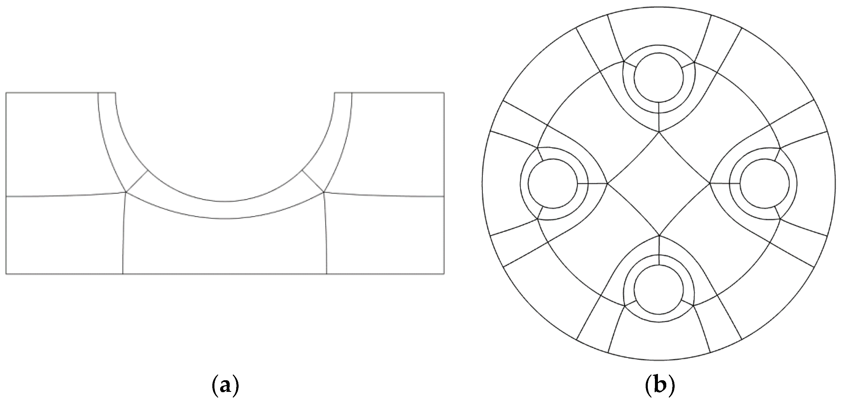
Figure 10a,c present the background triangular mesh of a model with the concave topology and four-hole topology, respectively. To be consistent with the input of the neural network, the number of mesh nodes is limited to around 2048 for each mesh. The corresponding frame fields of these two models are shown in Figure 10b,d. The singular structures of these two models obtained with the method introduced in Ref [10] can be seen in Figure 11a,b, respectively. Note that for the training of the neural network, a data set with the size of 2000 for each topology is created (seen in Table 2), among which 80% of the samples are used as the training set, and the remaining 20% are used as the testing set. Table 2 shows the accuracy and IoU of the training results on the testing sets. As can be seen, the overall accuracy rate exceeds 0.96, and the IoU exceeds 0.82.
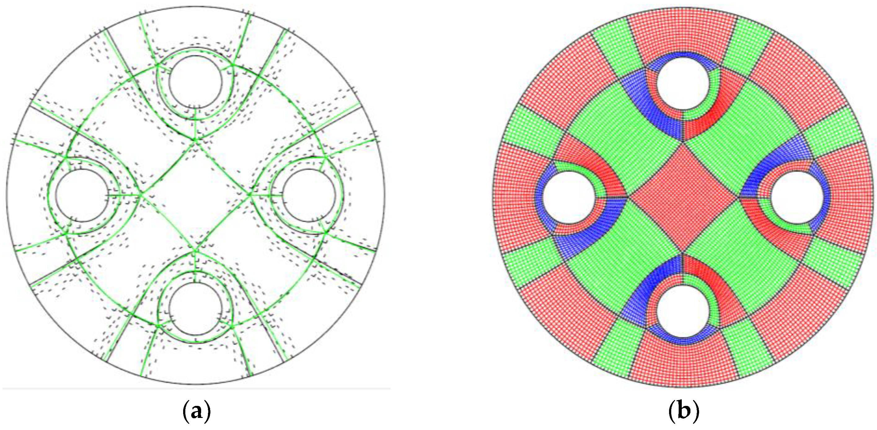
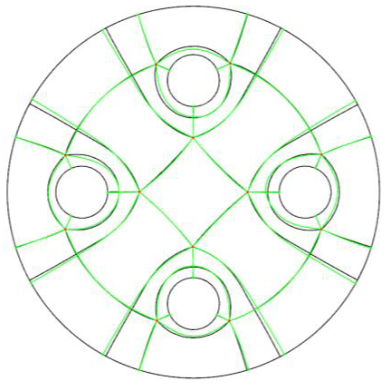
Figure 12a and Figure 13a present the prediction results of the concave model and the four-hole model shown in Figure 10, respectively. The short lines in the figure are the vectors of the frame component predicted by the neural network, which is around and aligned with the extension direction of the singular edges. These vectors are all located on the background mesh nodes, and these mesh nodes form several strips of the point cloud. It can be seen that the strips of point cloud almost go along with the extension direction of the singular edge of the model, and the directions of the vectors labeled with tag 1 are also almost consistent with the extension direction of the singular edge. The previous results mean that the convolutional neural network proposed in Section 3.1 can learn the distributions of the singular structures according to the input of frame field information. The green curves in Figure 12a and Figure 13a show the streamlines extracted from the predictions for the two geometric models. It can be seen that the domain decomposition results are quite close to the results obtained with the method in Ref. [10] shown in Figure 11a,b. This can be further verified in Figure 14 where the domain decomposition results generated by the proposed method and the method in Ref. [10] are presented together; it can be seen that only minor differences exist. The final block-structured quadrilateral mesh of the concave model and the four-hole model is shown in Figure 12b and Figure 13b, respectively.
In order to show the time efficiency of the proposed method, the four-circle model is used as an example to evaluate the time consumed during the step of domain decomposition with the proposed method and the method in Ref. [10]. The test is conducted on a personal computer (CPU: 3.5 GHz; Memory: 16 GB). With the predicted results of the CNN model, it takes 0.782 s for the proposed method to reconstruct the streamlines and obtain the domain decomposition result. However, the method in Ref. [10] consumes more than two times the time, i.e., 1.644 s, to generate the streamlines for domain decomposition. This is because the method in Ref. [10] relies on a numerical method to generate the streamlines, which is time consuming and could cause robustness issues. It needs to be noted that the proposed method needs extra time to train the CNN model, but for engineering designs that often require local modifications of the geometric model, the extra time can be apportioned to different design cycles.

6. Conclusions

The frame field distributed inside the model region describes the singular structural features inside the model. Aiming at the block-structured mesh generation problem, this paper proposes a convolutional neural network model to identify the internal singular structures contained in the frame field and then decompose the model area into multiple quadrilateral structures according to these singular structures and generate a block-structured quadrilateral mesh. The neural network model is trained with a large amount of model domain decomposition data. For geometric models with the same topology, the trained model can identify the frame component vectors located near the region segmentation streamlines and then construct the segmentation streamlines from the labeling results through an algorithmic process. Experiments show that the neural network model in this paper can effectively identify the internal singular structure of the model in order to realize the decomposition of the model area and the generation of block structure mesh.
Note that the proposed method can be extended to three-dimensional problems by considering one more frame component. The preparation of the training data and the network model would be similar to those in the two-dimensional problems. We will work on this extension in the near future. Finally, it needs to be mentioned that, currently, the network needs to be trained for each different topology structure.

Author Contributions

Conceptualization, Y.Z., X.C., Z.X. and G.X.; methodology, Y.Z., X.C. and Q.Z.; validation, Y.Z., X.C. and Q.Z.; writing—original draft preparation, Y.Z., X.C. and Z.X.; writing—review and editing, Z.X. and G.X. All authors have read and agreed to the published version of the manuscript.

Funding

This research received no external funding.

Institutional Review Board Statement

Not applicable.

Informed Consent Statement

Not applicable.

Data Availability Statement

Not applicable.

Conflicts of Interest

The authors declare no conflict of interest.

References

  1. Baker, T.J. Mesh generation: Art or science? Prog. Aerosp. Sci. 2005, 41, 29–63. [Google Scholar] [CrossRef]
  2. Bommes, D.; Lévy, B.; Pietroni, N.; Puppo, E.; Silva, C.; Tarini, M.; Zorin, D. Quad-mesh generation and processing: A survey. Comput. Graph. Forum 2013, 32, 51–76. [Google Scholar] [CrossRef]
  3. Bunin, G. A continuum theory for unstructured mesh generation in two dimensions. J. Comput. Aided Geom. Des. 2008, 25, 14–40. [Google Scholar] [CrossRef]
  4. Sun, L.; Armstrong, C.G.; Robinson, T.T.; Papadimitrakis, D. Quadrilateral multiblock decomposition via auxiliary subdivision. J. Comput. Des. Eng. 2021, 8, 871–893. [Google Scholar] [CrossRef]
  5. Zheng, Z.; Gao, S.; Shen, C. A progressive algorithm for block decomposition of solid models. Eng. Comput. 2022, 38, 4349–4366. [Google Scholar] [CrossRef]
  6. Fang, X.; Bao, H.; Tong, Y.; Desbrun, M.; Huang, J. Quadrangulation through morse-parameterization hybridization. ACM Trans. Graph. (TOG) 2018, 37, 1–15. [Google Scholar] [CrossRef]
  7. Fogg, H.J.; Armstrong, C.G.; Robinson, T.T. Automatic generation of multiblock decompositions of surfaces. J. Numer. Methods Eng. 2015, 101, 965–991. [Google Scholar] [CrossRef]
  8. Kowalski, N.; Ledoux, F.; Frey, P. Automatic domain partitioning for quadrilateral meshing with line constraints. J. Eng. Comput. 2015, 31, 1–17. [Google Scholar] [CrossRef]
  9. Jezdimirovic, J.; Chemin, A.; Remacle, J.F. Mul-ti-block decomposition and meshing of 2D domain using Ginzburg–Landau PDE. In Proceedings of the 28th International Meshing Roundtable, Buffalo, NY, USA, 14–17 October 2019. [Google Scholar]
  10. Xiao, Z.; He, S.; Xu, G.; Chen, J.; Wu, Q. A boundary element-based automatic domain partitioning approach for semi-structured quad mesh generation. Eng. Anal. Bound. Elem. 2020, 113, 133–144. [Google Scholar] [CrossRef]
  11. Li, N.; Shen, Q.; Song, R.; Chi, Y.; Xu, H. MEduKG: A Deep-Learning-Based Approach for Multi-Modal Educational Knowledge Graph Construction. Information 2022, 13, 91. [Google Scholar] [CrossRef]
  12. Hayat, A.; Morgado-Dias, F.; Bhuyan, B.P.; Tomar, R. Human Activity Recognition for Elderly People Using Machine and, Deep Learning Approaches. Information 2022, 13, 275. [Google Scholar] [CrossRef]
  13. Heidari, A.; Jamali MA, J.; Navimipour, N.J.; Akbarpour, S. A QoS-Aware Technique for Computation Offloading in IoT-Edge Platforms Using a Convolutional Neural Network and Markov Decision Process. IT Prof. 2023, 25, 24–39. [Google Scholar] [CrossRef]
  14. Heidari, A.; Navimipour, N.J.; Jamali MA, J.; Akbarpour, S. A green, secure, and deep intelligent method for dynamic IoT-edge-cloud offloading scenarios. Sustain. Comput. Inform. Syst. 2023, 38, 100859. [Google Scholar] [CrossRef]
  15. Bhatt, J.; Hashmi, K.A.; Afzal, M.Z.; Stricker, D. A survey of graphical page object detection with deep neural networks. Appl. Sci. 2021, 11, 5344. [Google Scholar] [CrossRef]
  16. Wu, Z.; Song, S.; Khosla, A.; Yu, F.; Zhang, L.; Tang, X.; Xiao, J. 3d shapenets: A deep representation for volumetric shapes. In Proceedings of the IEEE Conference on Computer Vision and Pattern Recognition, Boston, MA, USA, 7–12 June 2015; pp. 1912–1920. [Google Scholar]
  17. Maturana, D.; Scherer, S. Voxnet: A 3d convolutional neural network for real-time object recognition. In Proceedings of the 2015 IEEE/RSJ International Conference on Intelligent Robots and Systems (IROS), Hamburg, Germany, 28 September–2 October 2015; pp. 922–928. [Google Scholar]
  18. Riegler, G.; Ulusoy, A.O.; Geiger, A. Octnet: Learning deep 3d representations at high resolutions. In Proceedings of the IEEE Conference on Computer Vision and Pattern Recognition, Honolulu, HI, USA, 21–26 July 2017; p. 3577. [Google Scholar]
  19. Wang, P.S.; Liu, Y.; Guo, Y.X.; Sun, C.Y.; Tong, X. O-cnn: Octree-based convolutional neural networks for 3d shape analysis. ACM Trans. Graph. 2017, 36, 72. [Google Scholar] [CrossRef]
  20. Qi, C.R.; Su, H.; Mo, K.; Guibas, L.J. Pointnet: Deep learning on point sets for 3d classification and segmentation. In Proceedings of the IEEE Conference on Computer Vision and Pattern Recognition, Honolulu, HI, USA, 21–26 July 2017; pp. 652–660. [Google Scholar]
  21. Qi, C.R.; Yi, L.; Su, H.; Guibas, L.J. Pointnet++: Deep hierarchical feature learning on point sets in a metric space. Adv. Neural Inf. Process. Syst. 2017, 30, 1–10. [Google Scholar]
  22. Feng, Y.; Feng, Y.; You, H.; Zhao, X.; Gao, Y. Meshnet: Mesh neural network for 3d shape representation. Proc. AAAI Conf. Artif. Intell. 2019, 33, 8279–8286. [Google Scholar] [CrossRef]
  23. Wang, Y.; Sun, Y.; Liu, Z.; Sarma, S.E.; Bronstein, M.M.; Solomon, J.M. Dynamic graph cnn for learning on point clouds. ACM Trans. Graph. 2019, 38, 1–12. [Google Scholar] [CrossRef]
  24. Yao, S.; Yan, B.; Chen, B.; Zeng, Y. An ANN-based element extraction method for automatic mesh generation. Expert Syst. Appl. 2005, 29, 193–206. [Google Scholar] [CrossRef]
  25. Wang, N.; Lu, P.; Chang, X.; Zhang, L. Preliminary investigation on unstructured mesh generation technique based on advancing front method and machine learning methods. Chin. J. Theor. Appl. Mech. 2021, 53, 740–751. [Google Scholar]
  26. Wang, N.; Lu, P.; Chang, X.; Zhang, L.; Deng, X. Unstructured mesh size control method based on artificial neural network. Chin. J. Theor. Appl. Mech. 2021, 53, 2682–2691. [Google Scholar]
  27. Milletari, F.; Navab, N.; Ahmadi, S.A. V-net: Fully convolutional neural networks for volumetric medical image segmentation. In Proceedings of the 2016 Fourth International Conference on 3D Vision (3DV), Stanford, CA, USA, 25–28 October 2016; pp. 565–571. [Google Scholar]
  28. E. Bernhardsson Annoy at GitHub. Available online: https://github.com/spotify/annoy (accessed on 30 September 2020).
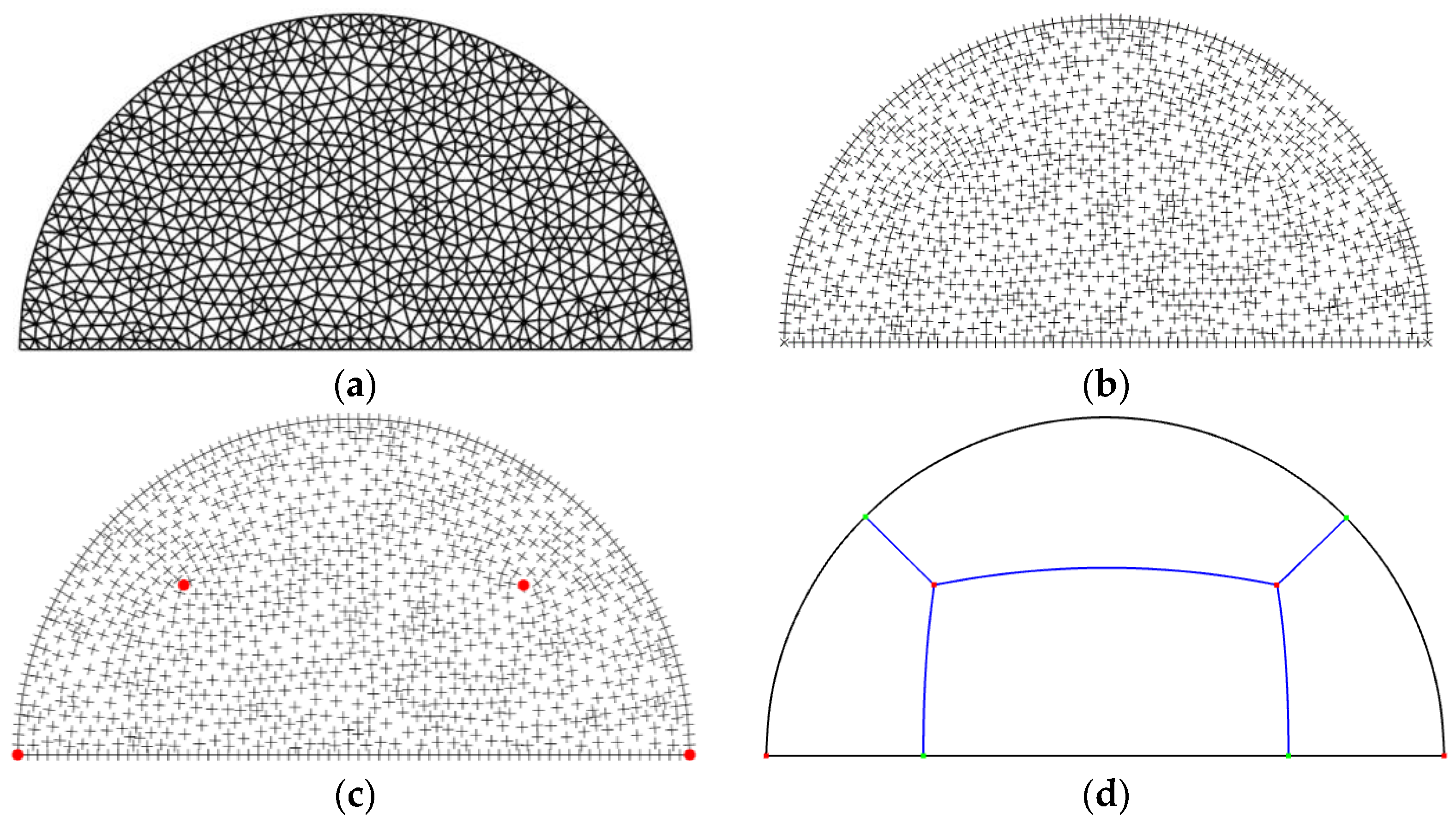
Figure 1. Domain decomposition based on frame field: (a) The background mesh; (b) The frame field; (c) The singular points in the frame field; and (d) The domain decomposition results partitioned by streamlines (lines in blue).
Information 14 00273 g001
Figure 2. A two-dimensional frame represented by: (a) Four vectors; and (b) Two perpendicular vectors, respectively.
Information 14 00273 g002
Figure 3. The vector component is annotated with label 1 (the arrow in red) if it is on the nodes of an element that is passed through by a streamline and it is consistent with the direction of the streamline.
Information 14 00273 g003
Figure 4. Labeled vectors of frames: (a) The background mesh and streamlines; (b) Vectors of frames that are marked with label 1.
Information 14 00273 g004
Figure 5. Part of the training data for the concave model.
Information 14 00273 g005aInformation 14 00273 g005b
Figure 6. Convolutional neural network architecture for labeling singular structure in frame fields.
Information 14 00273 g006
Figure 7. The workflow of the proposed method.
Information 14 00273 g007
Figure 8. Schematic of searching for the next node of the streamline: the nodes in black are the nodes already added to the streamline, the nodes in blue are the candidate neighboring nodes of s c , and the node in yellow is the next node of the streamline, the arrows are the frame components marked with label 1.
Information 14 00273 g008
Figure 9. Streamline extraction and quadrilateral mesh generation: (a) The extracted streamlines and the domain decomposition result; (b) The final block-structured quadrilateral mesh.
Information 14 00273 g009
Figure 10. The concave and four-hole models: (a,b) The background triangular mesh of a geometric model with the concave topology and the corresponding frame field; (c,d) The background triangular mesh of a geometric model with the concave topology and the corresponding frame field.
Information 14 00273 g010
Figure 11. Singular structures generated based on the method in Ref [10]: (a) A geometric model with the concave topology; (b) A geometric model with the four-hole topology.
Information 14 00273 g011
Figure 12. The concave model: (a) The vectors predicted with label 1 and the extracted streamlines; (b) The block-structured quadrilateral mesh.
Information 14 00273 g012
Figure 13. The four-hole model: (a) The vectors predicted with label 1 and the extracted streamlines; (b) The block-structured quadrilateral mesh.
Information 14 00273 g013
Figure 14. The domain decomposition results with the proposed method (streamlines in green color) and the method in Ref. [10] (streamlines in black color).
Information 14 00273 g014
Table 1. Detailed parameters of the convolutional neural network model.
LayersInputChannelsKernelStridePaddingOutput
Conv1[4,2048,4,1]16[1,1,1,16][1,1,1,1]VALID[4,2048,4,16]
Edge Conv1[4,2048,10,4]16[1,1,1,16][1,1,1,1]VALID[4,2048,10,16]
Concat1[4,2048,16,16]----------
Conv2[4,2048,16,1]32[1,1,1,32][1,1,1,1]VALID[4,2048,16,32]
Edge Conv2[4,2048,10,16]32[1,1,1,32][1,1,1,1]VALID[4,2048,10,32]
Concat2[4,2048,36,32]----------
Conv3[4,2048,32,1]64[1,1,1,64][1,1,1,1]VALID[4,2048,32,64]
Edge Conv3[4,2048,10,32]64[1,1,1,64][1,1,1,1]VALID[4,2048,10,32]
Concat3[4,2048,42,64]----------
Concat4[4,2048,1,112]----------
Max pool[4,2048,1,112]--[1,2048,1,1]----[4,1,1,512]
Expand[4,1,1,512]--------[4,2048,1,512]
Conv4[4,2048,1,512]256[1,1,512,256][1,1,1,1]VALID[4,2048,1,256]
Droupout[4,2048,1,256]----------
Conv5[4,2048,1,256]256[1,1,256,256][1,1,1,1]VALID[4,2048,1,256]
Droupout[4,2048,1,512]----------
Conv6[4,2048,1,256]128[1,1,512,128][1,1,1,1]VALID[4,2048,1,128]
Conv7[4,2048,1,128]2[1,1,128,2][1,1,1,1]VALID[4,2048,1,2]
Squeeze[4,2048,1,2]----------
Table 2. Training results of two two-dimensional examples.
Topology NameData SizeIoUAccuracy
The concave topology20000.8520.981
The four-hole topology20000.8210.965
Disclaimer/Publisher’s Note: The statements, opinions and data contained in all publications are solely those of the individual author(s) and contributor(s) and not of MDPI and/or the editor(s). MDPI and/or the editor(s) disclaim responsibility for any injury to people or property resulting from any ideas, methods, instructions or products referred to in the content.