A Hybrid Univariate Traffic Congestion Prediction Model for IoT-Enabled Smart City

Abstract

IoT devices collect time-series traffic data, which is stochastic and complex in nature. Traffic flow prediction is a thorny task using this kind of data. A smart traffic congestion prediction system is a need of sustainable and economical smart cities. An intelligent traffic congestion prediction model using Seasonal Auto-Regressive Integrated Moving Average (SARIMA) and Bidirectional Long Short-Term Memory (Bi-LSTM) is presented in this study. The novelty of this model is that the proposed model is hybridized using a Back Propagation Neural Network (BPNN). Instead of traditionally presuming the relationship of forecasted results of the SARIMA and Bi-LSTM model as a linear relationship, this model uses BPNN to discover the unknown function to establish a relation between the forecasted values. This model uses SARIMA to handle linear components and Bi-LSTM to handle non-linear components of the Big IoT time-series dataset. The “CityPulse EU FP7 project” is a freely available dataset used in this study. This hybrid univariate model is compared with the single ARIMA, single LSTM, and existing traffic prediction models using MAE, MSE, RMSE, and MAPE as evaluation indicators. This model provides the lowest values of MAE, MSE, RMSE, and MAPE as 0.499, 0.337, 0.58, and 0.03, respectively. The proposed model can help to predict the vehicle count on the road, which in turn, can enhance the quality of life for citizens living in smart cities.

1. Introduction

IoT has brought a lot of development to smart cities, which in turn increased road traffic. The transportation system is one of the basic necessities for a nation. It is a major factor that decides national economy. A nation considers traffic congestion as a threat to its economic growth. Traffic congestion also causes unnecessary delays for people while reaching their destinations. To manage traffic, a smart traffic congestion control system is needed [1]. That is why traffic congestion prediction has gained the attention of researchers to study and find a solution for this problem.

Various traffic stakeholders such as government agencies, traffic managers, city architects and planners, road users, policy makers, etc., get the benefit of traffic congestion management. Traffic congestion management helps to reduce time travel, increases road capacity, and makes roads safe to travel. Traffic congestion forecasting removes problems such as air pollution, noise pollution, fuel consumption, etc., which further helps to maintain a sustainable environment [2]. All these reasons are enough for a researcher to work in the field of traffic congestion forecasting, so that one can contribute to society.

In smart cities, roads have smart IoT sensors placed on both sides that collect data and send it to the storage space. A complete communication and data transfer system is shown in Figure 1. As shown in Figure 1, different sensors are placed near the road and send data to the message units. These message units are further connected to the IoT platforms using wireless networks. This IoT platform is connected to the central server. The central server handles the connection between the database server and storage units. All components can communicate using Wi-Fi. These sensors can be used to measure the speed of the vehicle, control traffic lights, and predict traffic congestion. Google Maps or Apple Maps also use real-time data gathered from IoT sensory devices to accurately predict and manage traffic congestion [3].

Smart wireless IoT sensors are used to calculate traffic flow, predict traffic congestion and control traffic routes. Two types of IoT sensor are used to handle real-time traffic problems, i.e., intrusive and non-intrusive. Intrusive sensors are placed on the pavements of roads that provide more accurate results, but they have high installation and maintenance cost. Piezoelectric, magnetic sensors, inductive loop detectors (ILD), and pneumatic road tubes are some of examples of intrusive sensors used for traffic data collection. Non-intrusive sensors are placed in different places on the road. These sensors are expensive and can be affected by environmental conditions. RFID (radio-frequency identification), ultrasonic, infrared, radar sensors, acoustic array sensors, video cameras, and road surface condition sensors are some of the examples of non-intrusive sensors [4].

Data collected using different IoT sensors are used for analysis and prediction using different Machine Learning (ML) or Deep Learning (DL) models. ML/DL models can provide insight from data captured by IoT devices using diagnostic, descriptive, predictive, and perspective analysis techniques [5]. ML/DL models help to predict or estimate traffic flow with accuracy. This helps to address the problem of traffic congestion in smart cities, which further assists people in decision-making while travelling.

Predictive analytics is a vital part of smart society because it helps in decision-making concerning the results. Machine learning and deep learning techniques can do wonders to gain insights from any kind of data such as structured, unstructured, or semi-structured [6]. Smart cities have many application areas such as parking space prediction, traffic congestion/flow prediction, etc. where predictive analytics can be useful to make the life of common people easier. In this study, a traffic congestion predictive model is proposed using ARIMA and LSTM. To enhance the quality of results, a back-propagation algorithm is used for forecasting results. The contributions of this article are:

(a)

This paper discusses the detailed literature on traffic congestion prediction techniques and different time-series dataset handling techniques.

(b)

A novel univariate predictive model is proposed using SARIMA, Bi-LSTM, and back-propagation techniques, which is elaborated in a stepwise manner.

(c)

This study discusses the behavior of a big IoT time-series dataset.

(d)

The study outlines the comparative analysis of the proposed model with the existing ones.

The rest of the paper is organized as follows. Section 2 elaborates on the related literature review that helps to understand the related work that has been undertaken in this field. Section 3 explains all the basic predictive machine learning algorithms used to propose a new technique. Section 4 explains the details of the proposed model in a stepwise manner. It also specifies details of the dataset and the evaluation parameters used in implementation. Section 5 presents the results analysis of the proposed model. It also provides a comparative analysis of the proposed and existing models. The conclusion of the research study is given in Section 6.

2. Literature Review

An Intelligent Transportation System (ITS) can be used to predict traffic congestion [7]. ITS uses IoT sensory devices to capture large-scale premium-quality traffic data that can be further treated with advanced methods of machine learning and deep learning [8]. Usually, the traffic dataset comes under the category of a time-series dataset, which requires extra effort and care while analyzing it.

A.A. Kashyap et al. [2] gave a detailed review of traffic flow prediction models. The authors emphasize the use of Multi-Layer Neural Network (MLNN) techniques, i.e., deep neural networks, to get better output. A comparative analysis of RNN, CNN, ANN, sparce auto-encoder, and hybrid models is given with respect to different datasets. The Caltrans PeMS dataset is used to check the performance of optimizers such as RMSprop, Adam, sgd for LSTM, and the GRU model. This study concluded that the hybrid model can outperform other models with spatio-temporal correlations for traffic flow prediction.

N. Zafar et al. [9] presented an algorithm that can be used to combine heterogeneous data collected using sensors or other data sources. The authors have presented an exploratory data analysis using GRU, CNN, LSTM, and their hybrid combinations. The LSTM+GRU hybrid combination gave the best performance with 4.5% RMSE and 6.67% MAPE.M.

T. Sun et al. [10] proposed an online traffic flow prediction model using GAN (Generative Adversarial Network) by combining Bi-LSTM and CNN (Convolutional Neural Network). A real-time dataset is taken using IoT sensor devices at the intersection of Hongzehu Road and Qingnian Road in Suqian City, Jiangsu Province, China. This is a time-series dataset on which, first, Bi-LSTM is used as a generator and, then, CNN is applied as a discriminant. Mean Squared Error (MSE), Mean Absolute Error (MAE), and binary entropy are the performance parameters used to measure the losses formulated by predictive models. The proposed model is found to be better than the Bi-LSTM and ARIMA model prediction results.

S. Majumdar et al. [11] discussed different machine learning approaches to predict traffic congestion for smart cities to make them sustainable. A Long Short-Term Memory (LSTM) network is introduced in this study to predict traffic flow based on the speed of the traffic. LSTM uses sigmoid as an activation function. The authors have considered both univariate and multivariate models to calculate traffic congestion. This study widely distributed the traffic flow prediction models into three categories: traffic-model-based methods, statistical techniques, and machine learning models. Real-time data of a road in Buxton (UK) is used for the analysis of the proposed model.

X. Feng et al. [12] proposed a short-term traffic flow prediction model using an Adaptive Multi-kernel Support Vector Machine (AMSVM). This model considered spatiotemporal correlation in the time-series dataset to explore the linear and nonlinear components of a real-time dataset. The proposed model’s hyperparameters are tuned using the Particle Swarm Optimization (PSO) technique.

T. Bogaerts et al. [13] proposed a long-term traffic forecasting model using deep learning techniques. Both LSTM and graph CNN deep learning models are combined to predict traffic. LSTM is used to handle temporal features and graph CNN is used for the spatial feature of the dataset. The proposed model is trained on a 36.5 GB real-time dataset collected from sparse trajectory (GPS) in CSV format.

S. Neelakandan et al. [14] proposed an IoT-based traffic prediction algorithm named OWENN (Optimized Weight Elman Neural Network) algorithm for a smart city. The authors used an Intel 80,286 microprocessor to propose a model for traffic signal control. The proposed traffic prediction system is divided into five different phases, i.e., data collection from IoT sensors, feature engineering, classification, optimization, and traffic control system. The OWENN model proved its worth with 98.23% accuracy and a 96.69% F-score.

Aid A. Khan et al. [15] proposed a model named modeling smart road traffic congestion control using artificial back-propagation neural networks (MSR2C-ABPNN) for traffic congestion prediction using machine learning techniques. The authors used two layered feed-forward ANN (artificial neural network) deep learning method for prediction optimized by a back-propagation neural network. The developed model is trained and validated on the secondary dataset of “M1 junction 37 England”. The proposed model provides an accuracy of 97.56% and RMSE of 4.351×10⁻³.

V. Rajalakshmi et al. [16] proposed two hybrid models. The first is ARIMA + MLP (Multi-Layer Perceptron) and the second is ARIMA + RNN (Recurrent Neural Network). The authors used the UK highway dataset to train the model. MAE, MSE, RMSE, and R2 are the different parameters used to validate the model. Between the two proposed models, ARIMA + RNN outperforms all the existing models with 0.53 as MAE and 0.61 as MSE.

S. Lu. et al. [17] proposed a hybrid model using ARIMA and LSTM for traffic flow prediction. This proposed model is implemented on a dataset given by the British government. Mainly, three trunk highways, i.e., AL215, AL2206, and AL2292, are considered for analysis data. Only six months of data are taken from the dataset, i.e., from September 2014 to March 2015. The linear component of this time-series dataset is handled by the ARIMA model and the nonlinear component is handled by LSTM using a back-propagation neural network. This method performed better than the standalone ARIMA and LSTM models.

F. Tseng et al. [18] proposed a traffic congestion prediction algorithm for real-time big data. The authors proposed an SVM-based real-time highway traffic congestion prediction (SRHTCP) model that collects real-time data from a highway of Tiwan. Spouts and bolts are used in Apache Storm to handle the real-time dataset for prediction. This proposed model improved accuracy by 25.6%.

H. Yi et al. [19] presented the use of the Tensorflow package of Python for traffic flow prediction. The authors used the Traffic Performance Index (TPI) for logistic regression analysis. Various on-board devices are used to collect real-time data for analysis purposes. The limitation of this study is that it uses only 1% of daily traffic data because of limited memory.

M. Bernas [20] proposed two new strategies to handle and improve the working of Wireless Sensor Networks (WSN) for traffic monitoring purposes. One of these strategies is to use a single mobile sink, and another is to use multiple sinks. Sensors are exploited in regions of high traffic density and low traffic density. The proposed strategies have also reduced power consumption. In [21], the author presented a way to predict weather using VANET technology. The author used VANET and the GSM communication network to carry weather data, and the calculation of this collected data is left for a smart vehicle. A lane with a high volume of traffic provided better results.

M. Bernas et al. [22] proposed a hybridized wireless network. In this network, radio signals play an important role, which helps to detect and classify the traffic on the road. These radio signals are generated by Bluetooth beacons placed on both sides of the road. Random forest, K nearest neighbor, decision tree, logistic regression, support vector machine, and PNN are the machine learning algorithms used to classify and detect traffic. The results obtained through the experiment explained that random forest outperforms all the other machine learning algorithms with an accuracy above 97% while monitoring the road traffic. This literature survey implies that traffic congestion prediction is a very active area for researchers to work on as multiple problems can be solved by working on this single problem. If the problem of traffic congestion is removed, then it can help in making a sustainable air and noise-pollution-free environment. Moreover, it can help in growing the economy of the nation by reducing the unnecessary time consumption of citizens in traffic, saving fuel consumption, etc.

Zahid et al. [23] gave a short-term traffic speed prediction for different time horizons. The authors proposed a Fast Forest Quantile Regression (FFQR) algorithm using hyperparametric optimization to enhance the performance of the speed prediction system. FFQR is an ensemble learning technique that uses multiple regression tree structures.

Most of the existing research work has shown that there is a trend of handling the linear and nonlinear features of a time-series dataset using hybrid models of statistical models and machine learning models. Linear functions are handled by the statistical model ARIMA, and nonlinearity is handled by any deep learning model that contains a nonlinear activation function. These hybrid models are combined simply by adding their forecasted results. However, how one can be so sure that the forecasted values can be hybridized simply by linearly adding the forecasted values of linear and nonlinear models? This creates a doubtful situation and uncertainty that motivates the work in this direction. This research helps to reduce the error rate and also optimize the working of existing predictive models.

Table 1. Different models used for traffic congestion prediction.

S. No.	Reference	Dataset Used	Model	Performance Matrices
1	T. Sun et al. [10]	Real time-Time series	IGAN-TF (Bi-LSTM + CNN)	MAE, MSE
2	S. Majumdar et al. [11]	Real time-Time series	LSTM	Accuracy
3	T. Bogaerts et al. [13]	Real-time GPS Time series	Graph CNN + LSTM	MAE, MAPE, RMSE
4	S. Neelakandan et al. [14]	Time series	OWENN	Accuracy, F- score
5	Aid A. Khan et al. [15]	M1 junction 37 England	MSR2C-ABPNN	Accuracy, RMSE
6	V. Rajalakshmi et al. [16]	UK highway	ARIMA + MLP/ ARIMA + RNN	MAE, MSE, RMSE and R2
7	Lu. Saiqun et al. [17]	Three trunk highway dataset of England	ARIMA + LSTM using BPNN	MAE, MSE, RMSE, MAPE
8	N. Zafar et al. [9]	FCD data source (data collected by a company)	LSTM + GRU	RMSE, MAPE
9	M. Zahid et al. [24]	Real-time dataset of Ring Road, Bejing, China	Decision jungle, Local Deep SVM, MLP	F1 score, Accuracy

summarizes the literature review explained in this section.

3. Background

Time-series data forecasting is one of the most challenging prediction tasks that can be achieved using machine learning models such as ARIMA, deep learning models such as RNN, CNN, LSTM, etc., and Fb Prophet [25]. The proposed hybrid model consists of the following components, which are explained in this section.

3.1. SARIMA

Generally, traffic congestion/flow prediction techniques are categorized into three categories, i.e., parametric technique models, machine learning technique, and deep learning techniques. Parametric techniques cover the ARIMA model, regression models, and Kalman filter. Machine learning techniques include ANN, KNN, and SVM. Deep learning techniques that can be used for traffic congestion prediction are CNN, LSTM, Encoder, GRU, and different hybrid models [26].

Regression models are considered to be a great tool to handle a time-series dataset. The ARIMA (autoregressive integrated moving average) model is used to predict the dataset, which is nonseasonal but has some patterns. The SARMA model is used when the dataset has some seasonal properties. The SARIMAX model is used when datasets have seasonal properties, as well as exogenous variables. ARIMA uses ‘p’ as a parameter for autoregression (AR). In the autoregression model, the ARIMA model uses past regressive values in the time-series equation to predict the future. ARIMA uses ‘q’ as a parameter for moving average (MA). ‘q’ represents the moving average order of the model. ARIMA uses ‘d’ as a parameter for integration (I). ‘d’ represents the differencing required to make the time-series dataset stationary.

Along with the variables (p, d, and q) used in ARIMA, SARIMA also requires periodic seasonal cycle of the data, which is represented by ‘s’. Equation (1) represents the SARIMA output (Y_t).

$$Y_t=c+\sum _{n=1}^p{\alpha }_n{y}_{t-n}+\sum _{n=1}^q{\theta }_n{\in }_{t-n}+\sum _{n=1}^P{\varnothing }_n{y}_{t-sn}+\sum _{n=1}^Q{\eta }_n{\in }_{t-sn}+{\in }_t$$

(1)

where c is a constant factor, α and y are used to calculate autoregression for time t in the nonseasonal part, θ and ∈ are used to calculate moving average for time t in the nonseasonal part, ∅ and y are used to calculate autoregression for time t in the seasonal part (s), η and ∈ are used to calculate moving average for time t in the seasonal part (s)$,\mathrm{a}\mathrm{n}\mathrm{d}{\in }_t$ is an error term at time t.

3.2. Bi-LSTM

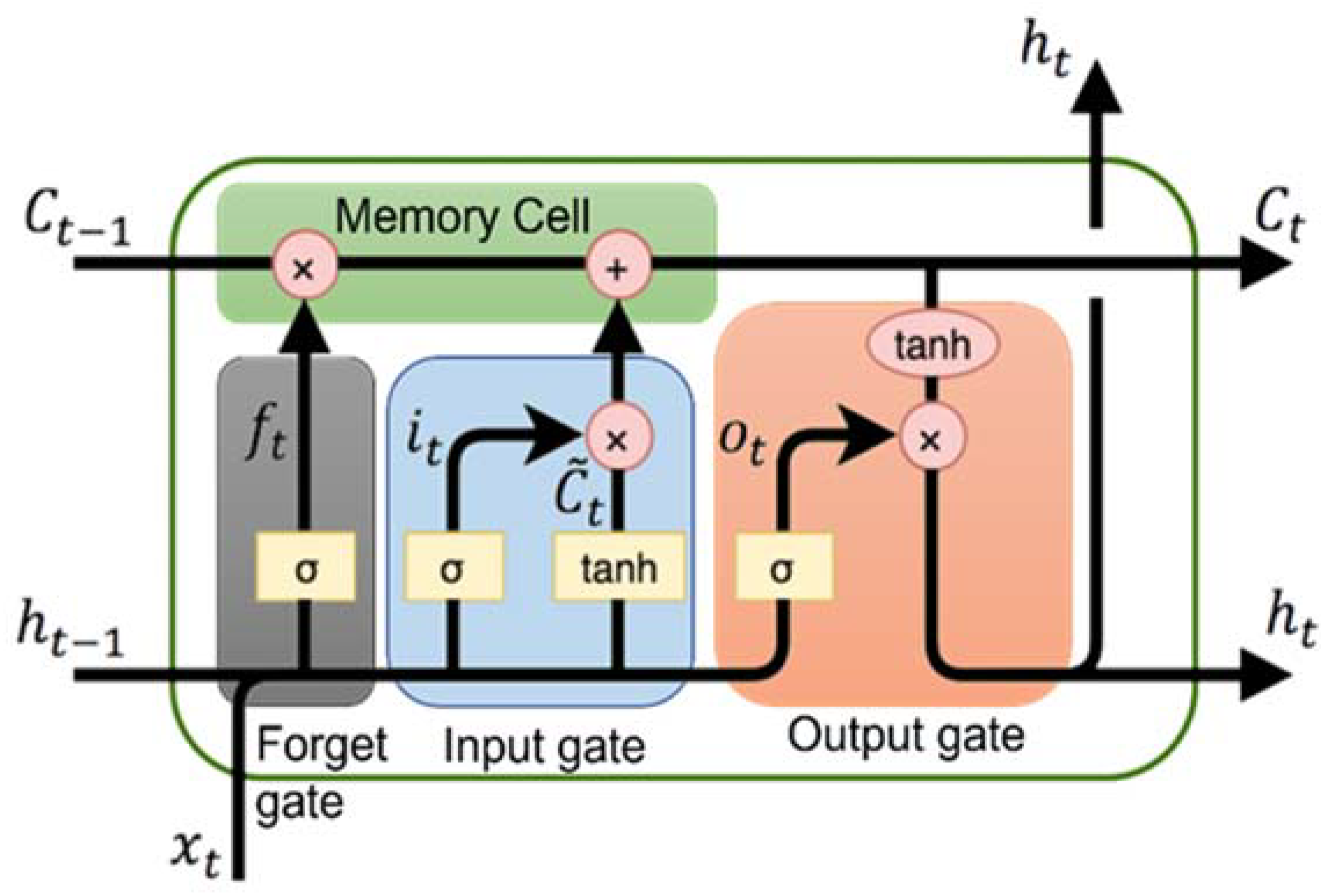
The Long Short-Term Model (LSTM) is an improved version of the RNN, which has some memory retention power. Figure 2 represents the basic architecture of LSTM. The LSTM model is divided into three basic gates called input gate, output gate, and forget gate. A memory cell plays an important role in retaining previous values [27]. The first layer is the forget layer, which decides on the data to be retained in the memory cell. Next is the input gate layer, which gives input to the LSTM network. It decides which data should be passed into the network and which data should be restricted outside the network. Last is the output layer. This layer decides which memory cell state is given as output [28].

Suppose, X {x₀, x₁, x₂, …….. x_t} is considered as input given to the LSTM model, and h{h₀, h₁, h₂, ……. h_t} is considered as output of the LSTM cell. Different gates of LSTM can be elaborated mathematically as follows:

Input gate:

$$i_t=\mathsf{\sigma }(W_{x_i}{x}_t+{\mathrm{W}}_{hi}{h}_{t-1}+{\mathrm{W}}_{ci}{c}_{t-1}+b_i)$$

(2)

Forget gate:

$$f_t=\mathsf{\sigma }(W_{x_f}{x}_t+W_{hf}{h}_{t-1}+{\mathrm{W}}_{cf}{c}_{t-1}+b_f)$$

(3)

Cell state:

$$c_t=f_t{\odot c}_{t-1}+i_t\odot \tanh (W_{x_c}{x}_t+{\mathrm{W}}_{hc}{h}_{t-1}+b_c)$$

(4)

Output gate:

$$o_t=\mathsf{\sigma }(W_{x_o}{x}_t+{\mathrm{W}}_{ho}{h}_{t-1}+{\mathrm{W}}_{co}{c}_{t-1}+b_o)$$

(5)

LSTM cell output:

$$h_t=o_t\odot \mathrm{t}\mathrm{a}\mathrm{n}\mathrm{h}\left(c_t\right)$$

(6)

where t = timestamp, x_t = input, i_t = input gate at time t (Equation (2)), f_t = forget gate at time t (Equation (3)), c_t = memory cell state at time t (Equation (4)), w = weight-matrix, o_t = output gate at time t (Equation (5)), and h_t = LSTM output at time t (Equation (6)).

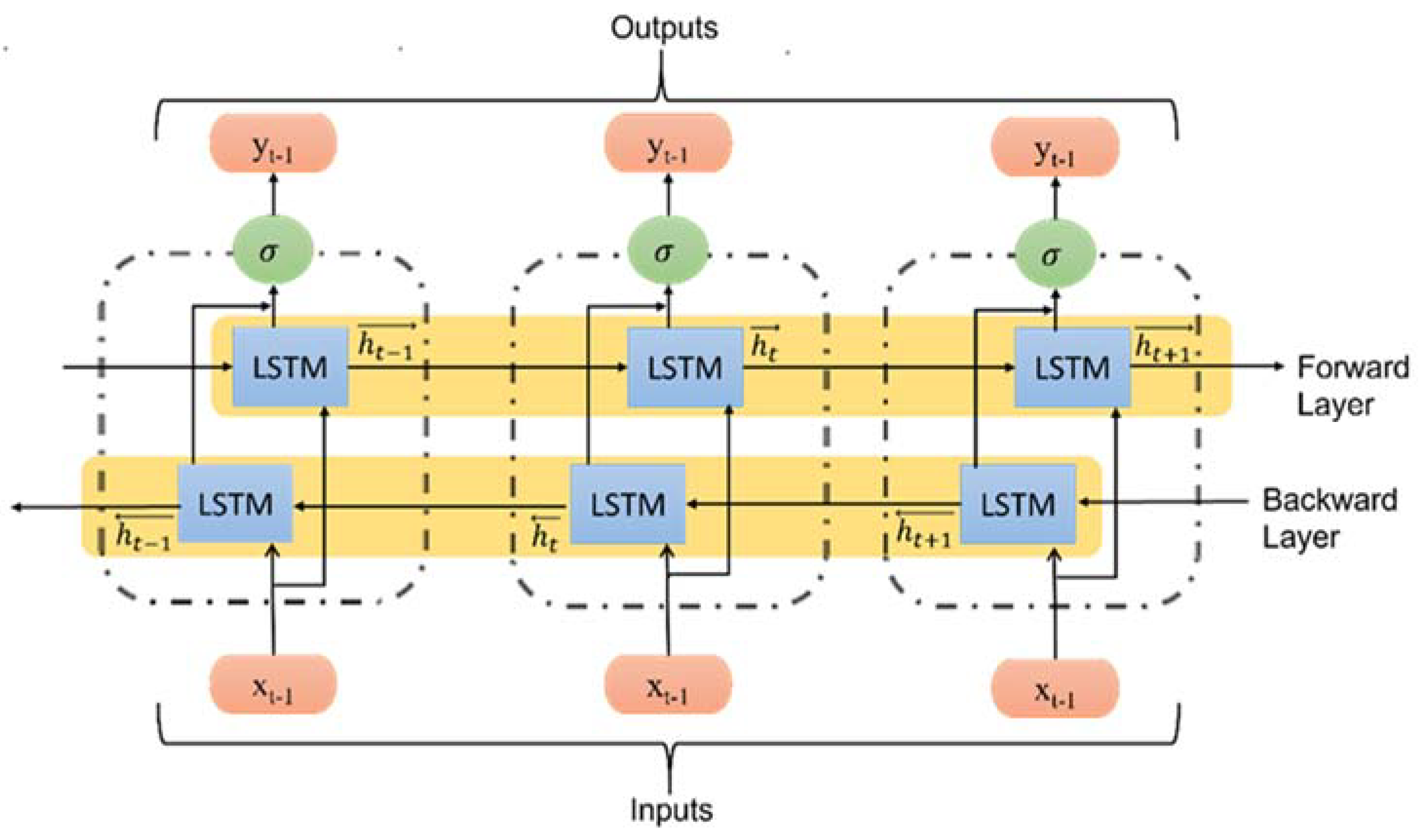
Bi-LSTM stands for bidirectional long short-term model. Bi-LSTM is an extended version of LSTM. The main disadvantage of LSTM is that it makes predictions using only past/previous values of the data. Future observations play no role in making decisions using LSTM. Bi-LSTM improves the predicted outcomes using both previous as well as future observations. In the Bi-LSTM model, data can flow in both the forward and backward directions. This helps the predictive model to use past data, as well as future data, to train the model and take appropriate actions. Both past observations and future results are stored in the memory cells, which helps in decision making [29]. Figure 3 shows the bidirectional LSTM architecture.

Suppose X{x₀, x₁, x₂,………..x_t} is considered as input given to the Bi-LSTM model and y{y₀, y₁, y₂,……… y_t} is considered as its output. Since data flows in both directions in the hidden layers of Bi-LSTM, $\overrightarrow{h}${$\overrightarrow{h_0},\overrightarrow{h_1},\overrightarrow{h_2},\dots \dots ,\overrightarrow{h_t}$} is considered as data flow in the forward direction and $\overleftarrow{h}${$\overleftarrow{h_0},\overleftarrow{h_1},\overleftarrow{h_2},\dots \dots ,\overleftarrow{h_t}$} is considered as data flowing in the backward direction. The predicted value at time t is represented as ‘y_t’ (given in Equation (9)), calculated by concatenating the data values of forward and backward flow. Mathematical representation of the Bi-LSTM model’s forward and backward dataflow is given in Equations (7) and (8) [30].

$$\overrightarrow{h_t}=\mathsf{\sigma }(W_{{\overrightarrow{h}}_x}{x}_t+W_{\overrightarrow{h}\overrightarrow{h}}{\overrightarrow{h}}_t+b_{\overrightarrow{h}})$$

(7)

$$\overleftarrow{h_t}=\mathsf{\sigma }(W_{{\overrightarrow{h}}_x}+W_{{\overleftarrow{h}}_x}+b_{\overrightarrow{h}})$$

(8)

$$y_t=W_{y\overrightarrow{h}}\overrightarrow{h}+W_{y\overleftarrow{h}}\overleftarrow{h}+b_y$$

(9)

where σ is a logistic sigmoid function, t is a time stamp, and b represents the bias function.

3.3. Back Propagation Neural Network

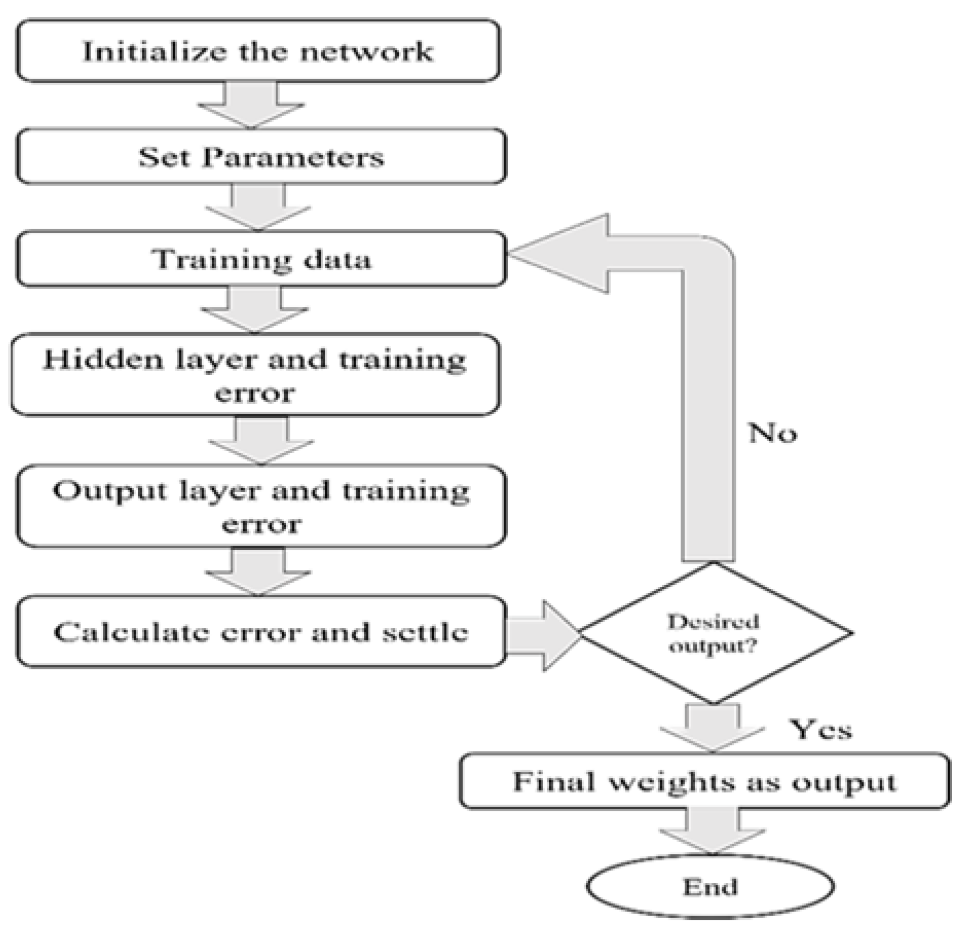
Back-Propagation Neural Networks (BPNNs) are most commonly used neural networks. The architecture of BPNNs consists of an input layer, one or more hidden layers, and an output layer. The main concept of the back-propagation technique is to send errors in a backward direction from the output layer to the hidden layers. This helps to tune the weights of the neurons, which reduces the error rate in the overall predicted result. BP is similar to a multi-layer feed-forward neural network using a backward error propagation algorithm [31]. The BP algorithm is made up of two basic steps: forward propagation and backward propagation. Figure 4 shows the workflow diagram of back propagation.

• In the first step, input values of the dataset are fed forward from the input layer, then to the hidden layers, and finally to the output layer.
• In the second step, output errors are calculated and then propagated in the backward direction of network. This step helps to tune different features of the neural network.
• These steps repeat until the desired output is achieved with a minimum error value.

4. Proposed Model and Implementation

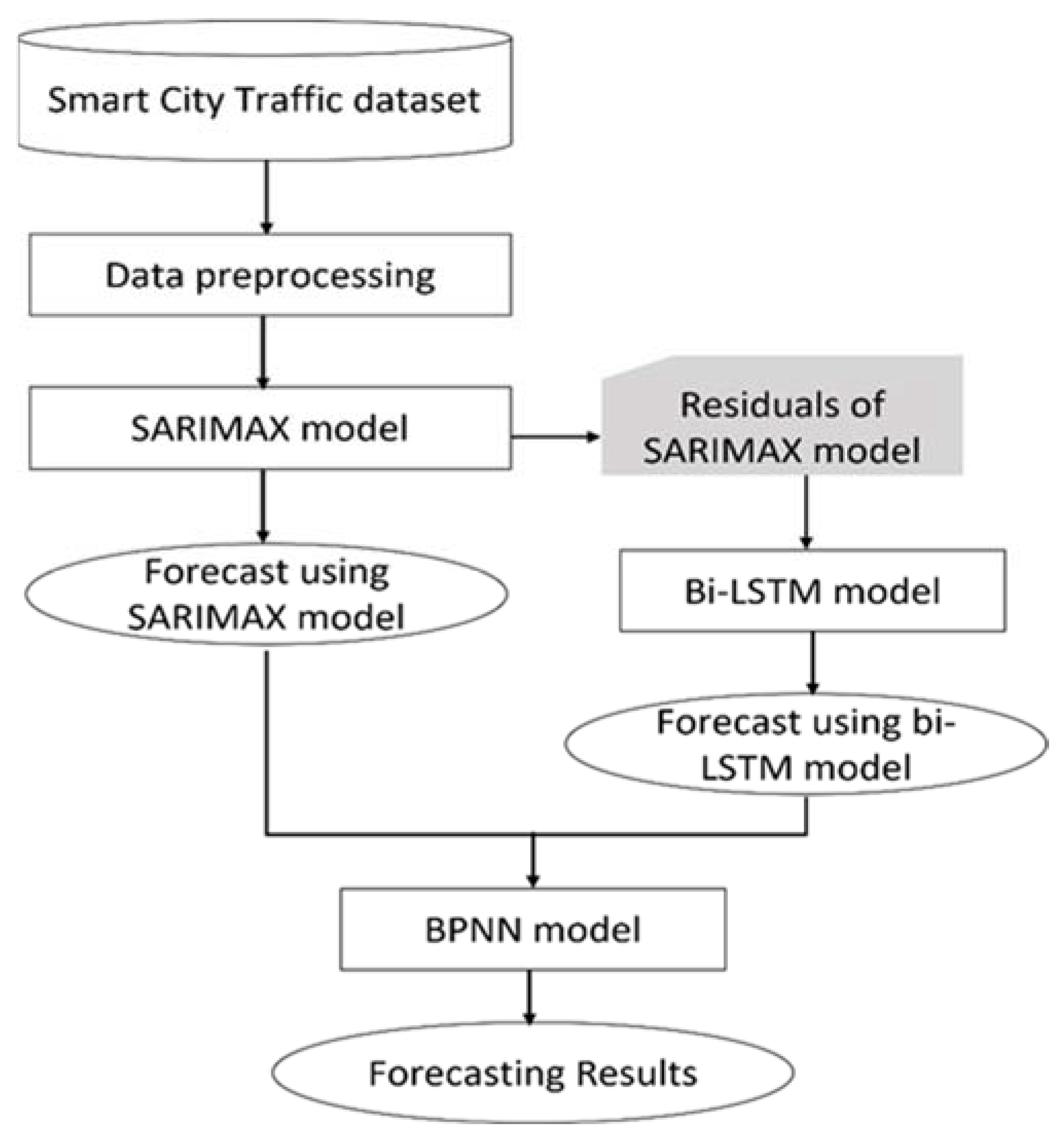
This study proposes a hybrid SARIMA + Bi-LSTM model optimized using BPNN to predict traffic congestion using a univariate time-series IoT dataset. The proposed hybrid model uses two prediction models: one is statistical and the other is a machine learning model. SARIMA, which is a statistical model, is used to train linear components of the dataset, and Bi-LSTM, which is a machine learning model, is used to train nonlinear values of the time-series IoT dataset. After training the linear and nonlinear values of the dataset, these predictive models are used for forecasting. Predicted results are then fed into the BPNN, which helps to readjust the neurons’ weights and reduces errors. The pseudocode of the proposed model is given in Algorithm 1.

Algorithm 1. Pseudocode of proposed model.

Input: Yt {y0,y1,y2,…….yi} = Timeseries dataset, i = number of time-series dataset instances Output: Predicted output Oh

Begin For each Yi of dataset Y Step 1: Data Preprocessing     ● Finding and removing null values     ● Set index as TIMESTAMP with frequency = D     ● Decompose dataset to check seasonality     ● Splitting Yt into Ytrain and Ytest

Step 2: SARIMA (Ytrain, Ytest) // handling linear components of Yt     ● Estimated differencing term d // use “pmdarima” package to calculate order of SARIMA model with minimum aic     ● auto_arima (Ytrain, seasonal=True, m=4, D=1, start_P=1, start_Q=1, max_P=5, max_Q=5,     ● information_criterion=‘aic’, trace=True, error_action=‘ignore’, stepwise=True) //use “pmdarima” package to forecast     ● ${\widehat{L}}_t$ = pmresults.forecast(Ytest)

Step 3: Calculating residuals     ● NLt = Yt–${\widehat{L}}_t$

Step 4: Preprocessing residuals     ● Find autocorrelation in residual values     ● Splitting residual values in NLtest, NLtrain, and NLvalidation data     ● Scaling residual values using minmaxscaler()

Step 5: Bi-LSTM (NLtrain) // handling nonlinear components of NLt     ● Set sequence size and number of features to be used for prediction // create a sequential stacked bi-lstm model using “Keras” package     ● Add two Bi-LSTM layer, a dropout layer and two dense layers     ● Add optimizer=Adam(learning_rate=0.01)     ● Compile model with loss=‘mean_squared_error’, metrics=[‘mse’,’mae’]     ● Fitting the model with 100 epochs // forecasting     ● ${\widehat{NL}}_t$ = predict(NLtest)

Step 6: BPNN (${\widehat{L}}_t$, ${\widehat{NL}}_t$, Yt) // forecasted values of SARIMA and Bi-LSTM are given as input to produce combined prediction values     ● Scale the predicted values of SARIMA and Bi-LSTM using minmaxscaler() // Initialize the network     ● Neural network is initialized with ${\widehat{L}}_t$, ${\widehat{NL}}_t$ as inputs, Yt as output, and three hidden layers // train the network     ● Calculate neuron activation for input     ● Activation function = 1.0/(1.0 + exp(-activation)) is used to find the correlation between ${\widehat{L}}_t$, ${\widehat{NL}}_t,$ Yt     ● Apply forward propagation with learning rate = 0.9, epochs = 5000     ● Calculate errors     ● Apply backward propagation to propagate and store errors in backward direction of the model     ● Update network weights with error     // Make a prediction with a network     ● ${\widehat{Y}}_t$ = predict(trained network, Yt)

Step 7: Evaluating model     ● Evaluate proposed model using MSE and MAE END

4.1. Algorithmic Steps for the Proposed Model

The flow chart of the working model is given in Figure 5. Algorithmic steps of the proposed hybrid model are explained as follows:

Step 1: Time-series dataset is comprised of a linear component (L_t) and nonlinear component (NL_t). In the first step, the IoT time-series dataset is decomposed using the “statsmodels” package of Python. This decomposition helps to check the seasonality, trend, and residual values of the feature used for predicting traffic congestion. Equation (10) gives the mathematical representation of the raw dataset (y_t).

$$y_t=L_t+{NL}_t$$

(10)

Step 2: Dataset is found to be seasonal, so linear components of the time-series IoT dataset are given to the SARIMA model. Equation (11) shows the predicted values of the SARIMA model (${\stackrel{-}{L}}_t$). The “pmdarima” package is used to choose the best parameters for SARIMA to forecast traffic congestion.

$${\widehat{L}}_t=SARIMA\left(y_t\right)$$

(11)

Step 3: Residual values (NL_t) of the SARIMA model are calculated as given in Equation (12) and given as input to the Bi-LSTM model.

$${NL}_t=y_t-{\widehat{L}}_t$$

(12)

Step 4: The Bi-LSTM model is used to handle the nonlinear component of the time-series IoT dataset given in Equation (13). Bi-LSTM generates the forecast values for nonlinear components.

$${\widehat{NL}}_t=Bi\text{\_}LSTM\left({NL}_t\right)$$

(13)

Step 5: Forecasting Values of SARIMA and Bi-LSTM are combined using BPNN. BPNN helps to find the unknown function “f”, which helps to combine the linear and nonlinear forecasting values, as given in Equation (14). BPNN also optimized the results by propagating error values backward in the neural network and optimizing the weights of the neurons in the forward direction.

$${\widehat{y}}_t=f({\widehat{L}}_t,{\widehat{NL}}_t)$$

(14)

Through the BPNN, the model can forecast ${\widehat{y}}_t$ values using forecasted results of SARIMA (${\widehat{L}}_t$) and Bi-LSTM (${\widehat{NL}}_t$). This model uses a back-propagation neural network to discover the real relationship function between SARIMA and Bi-LSTM forecasted values. The novelty of this model is that it does not speculate that forecasted values of SARIMA and Bi-LSTM can only be hybridized using the addition function only.

4.2. Dataset Used

For this research, the “CityPulse EU FP7 project” dataset is used [32]. This dataset is considered as big data collected using IoT sensor devices of the smart cities. It contains data of road traffic, weather, and pollution collected from smart cities, Aarhus of Denmark and Brasov of Romania. For this study, the road traffic dataset is chosen. The road traffic dataset for Aarhus city is collected over time in four different durations, i.e., from February 2014 to June 2014, from August 2014 to September 2014, from October 2014 to November 2014, and from July 2015 to October 2015 [33].

This dataset has a high-level smart city scenario, and this is a complete package of functional and nonfunctional components of a smart city framework that can be helpful or useless for data processing. A complete KPI (Key Performance Index) guide is given for the evaluation of the smart city framework dataset. Based on the functional component, the datasets provide three categories to measure them:

• Observational KPI: these KPIs are related to the observation points such as the virtual or physical environment near the sensors used, the environment nearby, and temporal constraints.
• Network connected KPI: these KPI are related to the kind of network used for the connection of the sensors, security measures to be taken for safe connection over the network, etc.
• Data-processing KPI: these KPIs are related to the computational capabilities of the smart city framework. It basically deals with the data processing that can take place inside the functional component of the framework.

To handle data processing KPIs, a road traffic dataset of the duration from February 2014 to June 2014 is used in this study. This smart city framework collected data for various locations within the city with respect to every single sensor device. The dataset contains the different features, as explained in

Table 2. Dataset description.

S. No.	Feature	Significance
1	Status	This feature gives the status report of the IoT sensor device used.
2	avgMeasuredTime	It gives average measured time.
3	avgSpeed	It gives the average speed of a vehicle for the given time.
4	medianMeasuredtime	It provides a median time for the sensor to measure speed and count.
5	TIMESTAMP	This feature gives the exact timestamp for which the vehicle counts and the average speed of the vehicle.
6	vehicleCount	It gives the number of vehicles on the street for a particular time interval.
7	_id	It gives the ID of a sensor device.
8	Report_id	Report ID gives the ID for a particular area location for which all the above features are observed.

.

4.3. Evaluation Matrices

Evaluation parameters are used to validate the model with respect to the dataset used. Evaluation parameters can be chosen according to the problem statement. Some researchers focus on the accuracy of the results and some focus on reducing the error rate in the model. For this study, error rate is considered as a parameter to evaluate the hybrid model. The proposed model is considered as best if it gives minimum error. Although there are different parameters such as Mean Squared Error (MSE), Mean Absolute Error (MAE), Root Mean Square Error (RMSE), etc., MSE, MAE, RMSE and MAPE are used as comparative and evaluating parameters for this study [34].

• Mean Squared Error (MSE): MSE is considered as the best parameter to check the error rate of the regression prediction model. The lower the value of MSE, the better the model is. MSE can be calculated as given in Equation (15):

  $$MSE=\frac{1}{n}{\sum }_{i=1}^n{\left({\mathrm{Y}}_i-{\mathrm{Y}}_i\right)}^2$$

  (15)

  where n denotes the number of data items, Y_i denotes the actual values, and Y_i represents the predicted value.
• Mean Absolute Error (MAE): MAE is the difference between the predicted values and the actual correct values but in the paired observation. These paired observations are considered to be the ones that are creating the same phenomenon. MAE can be calculated as given by Equation (16):

  $$MAE=\frac{{\sum }_{i=1}^n\left|y_i-x_i\right|}{n}$$

  (16)

  where n denotes the number of data items, y_i denotes the predicted values, and x_i represents actual correct values.
• Root Mean Squared Error (RMSE): RMSE represents absolute fit of the model with respect to the data. The lower the value of this parameter, the better the model is considered. It can be calculated as given in Equation (17).

  $$MSE=\sqrt{\frac{1}{n}{\sum }_{i=1}^n{\left({\mathrm{Y}}_i-{\mathrm{Y}}_i\right)}^2}$$

  (17)

  where n denotes the number of data items, Y_i denotes the actual values, and Ŷ_i represents the predicted value.
• Mean Absolute Percentage Error (MAPE): It is also called Mean Absolute Percentage Deviation (MAPD). It represents keeping track of relative errors with respect to the actual values in percentage. MAPE can be calculated as given in Equation (18):

  $$MAPE=\frac{1}{n}{\sum }_{i=1}^{n-1}\frac{\left|{\mathrm{Y}}_i-{\mathrm{Y}}_i\right|}{max\left(\mathcal{E},\left|{\mathrm{Y}}_i\right|\right)}$$

  (18)

  where n denotes the number of data items, Y_i denotes the actual values, Y_i represents the predicted value, and $ℰ$ is a small positive arbitrary value.

5. Results and Discussion

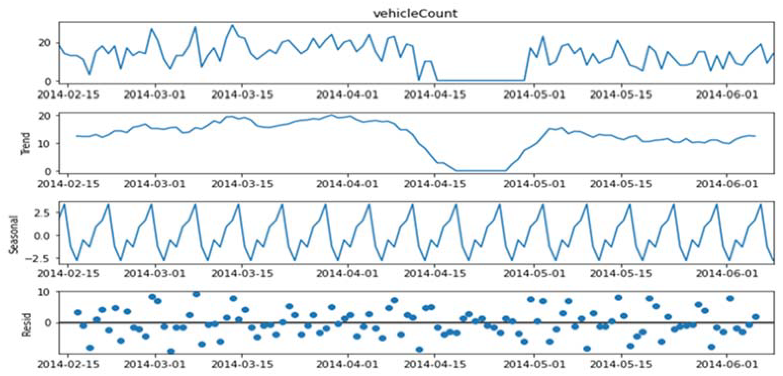
A big IoT dataset is used for this traffic congestion prediction research. At first, the dataset is decomposed to check its seasonality, trend, and residuals. This would help to decide the different pre-processing measures to be taken before data analysis. This decomposition helps us to decide which kind of ARIMA model is to be used, i.e., SARIMA, SARIMAX, SARMA, ARMA, etc. Figure 6 presents the decomposed result of the IoT dataset used for this study. Decomposition of the dataset shows that there is seasonality in the dataset but no trend. There are residual values present in the dataset also, which are to be handled with care.

After decomposition, the dataset is preprocessed and split into testing and training data. Before giving the dataset to the SARIMA model, periodicity of the data is adjusted to be quarterly. This testing and training dataset is given to the SARIMA model, which is used to handle the linear component of this seasonal dataset. The “auto_arima” function of the “pmdarima” package is used to calculate the best fit parameters that can be used for the prediction with the minimum AIC (Akaike Information Criterion) value. The “auto_arima” helps to parameterize SARIMA by choosing optimal values of (p, d, q) (P,Q,D,s). After running the auto_arima function on the training dataset, (p, d, q) (P,Q,D,s) came out to be (2, 0, 0) (0, 1, [1], 4) with a minimum AIC value of 520.055. Since it is quarterly data, the periodicity factor ‘s’ is 4.

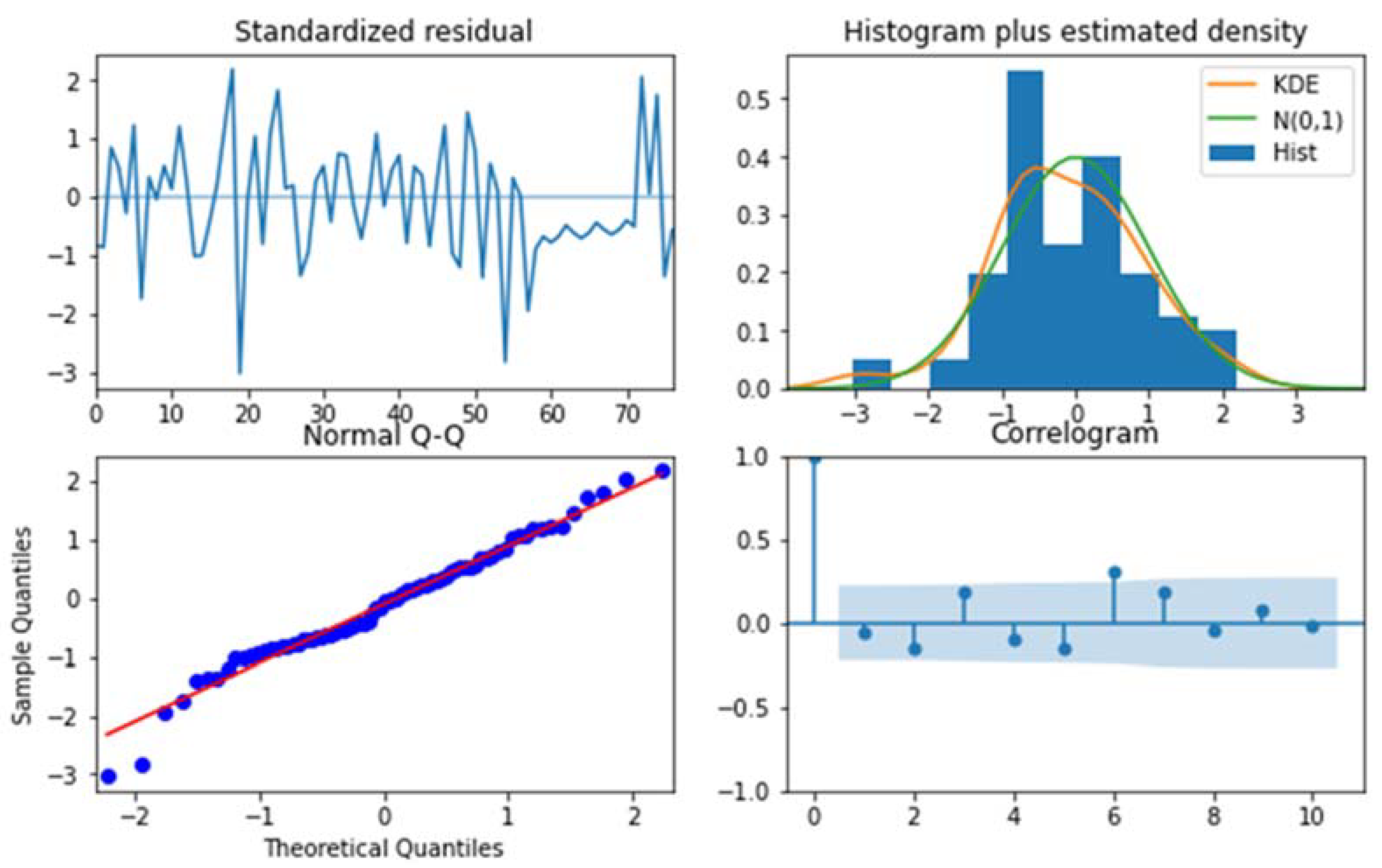
Figure 7 represents diagnostic results of the SARIMA model. Figure 7 presents standard residual plot, normal Q-Q plot, correlogram, and a histogram with estimated density. From a standardized residual plot, it can be seen that the residual errors are moving around zero mostly, which implies that chances of error for the linear component of the data is negligible. The histogram shows that it is a normal distribution curve that is centered at mean 0. Theoretical quantities and sample quantities are skewed in the normal Q-Q plot. Lastly, the correlogram represents the ACF values. The ACF plot represents that the similarities between residual values and their lagged version for the given time period are not correlated.

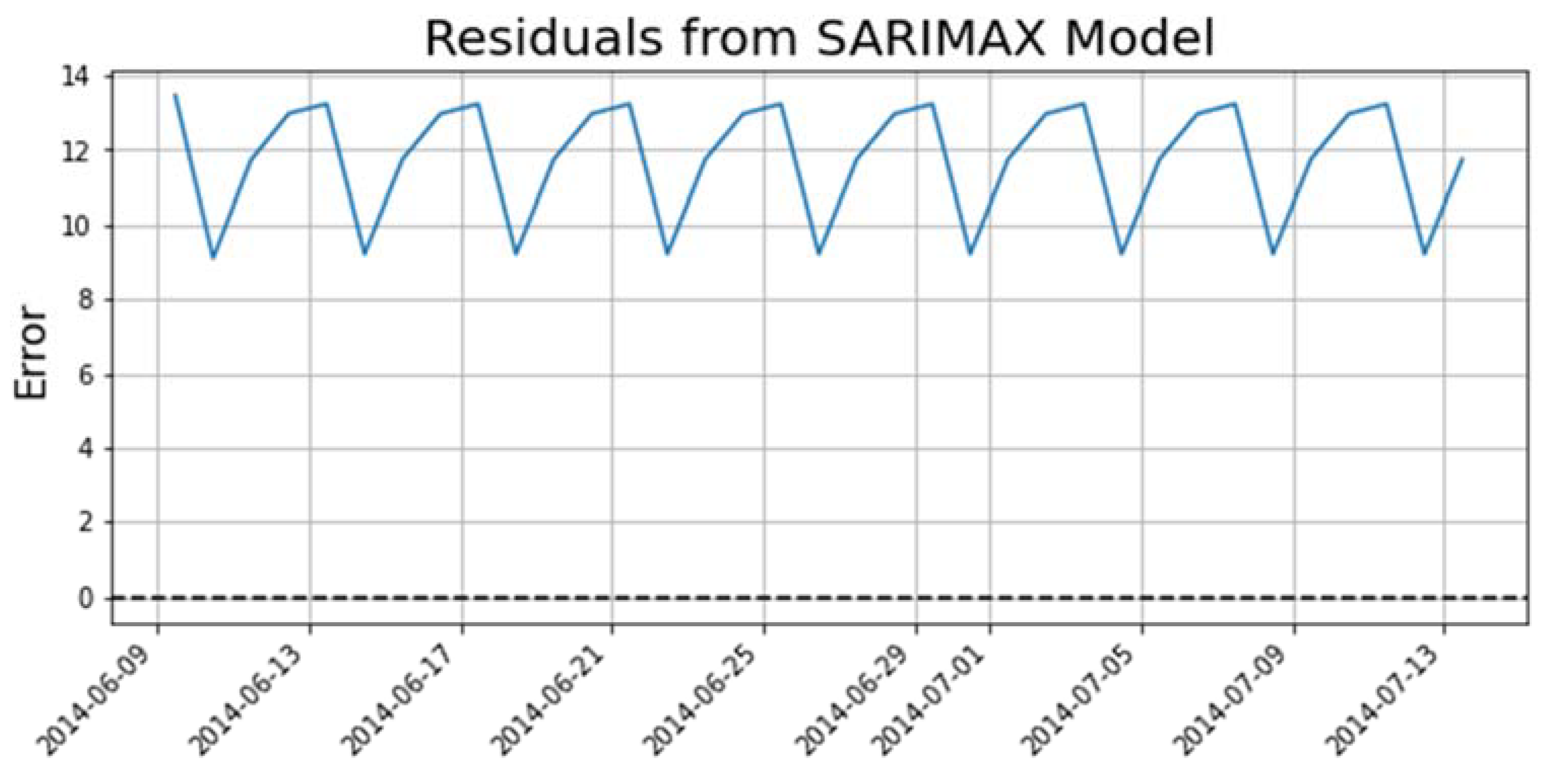
Figure 8 presents a comparative plot that shows the training dataset values, predicted values, and actual values. As seen in Figure 8, there are gaps between actual and forecasted values. To remove these gaps and reach more accurate data points, the Bi-LSTM model is used. The Bi-LSTM model will handle the nonlinear data points. So, residual values are given as input to the Bi-LSTM model. Figure 9 shows the residual values of the SARIMA model. Before applying the Bi-LSTM model, residual values of the SARIMA model are split into training, validation, and testing dataset. The ‘MinMaxScaler()’ function is then used to scale these residual values in the range of (−1,1). Scaled values help the model to get better results. These scaled values are then given to the Bi-LSTM model.

To implement the Bi-LSTM model, the “Keras” package is used. “Keras” is a Python-based platform for implementing deep learning modules on “tensor flow”. Using “Keras”, a stacked Bi-LSTM deep learning model is used to handle the nonlinear residual values of the dataset.

Table 3. Hyperparameters of Bi-LSTM model.

Hyper Parameter	Bi-LSTM
Optimizer	Adam
Learning rate	0.001
Activation function	Sigmoid (layer 1), tanh (layer 2)
Dropout rate	0.2
Epochs	100

shows the hyperparameter used in this stacked Bi-LSTM model. Bidirectional LSTM helps to minimize the error by handling past and future predictive values. The Adam optimizer [34] is used to optimize the Bi-LSTM model. The learning rate used is 0.01 for Adam. An optimizer is used to reduce the error rate. In the Bi-LSTM network, two layers of Bi-LSTM are used, having sigmoid and tanh activation functions for layer 1 and layer 2, respectively. Then, one dropout layer is also there, which has a 0.2 dropout rate. The Bi-LSTM deep learning model uses 100 epochs to reach minimum loss values.

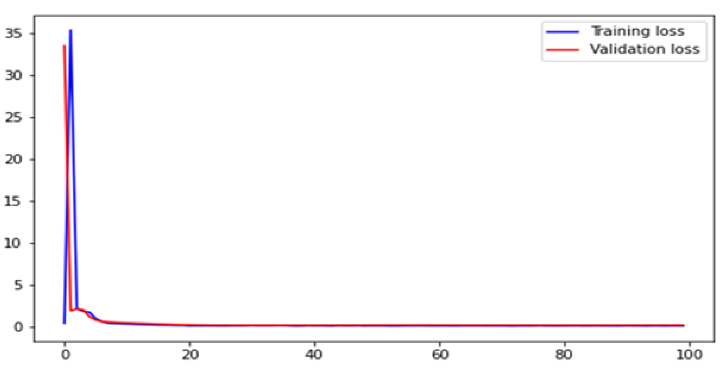
Figure 10 presents the loss between the training and validation data while modeling the dataset according to the Bi-LSTM model. It can be seen in Figure 10 that after applying the Bi-LSTM model on the training dataset, loss has been reduced. The loss became minimum as the epoch increased.

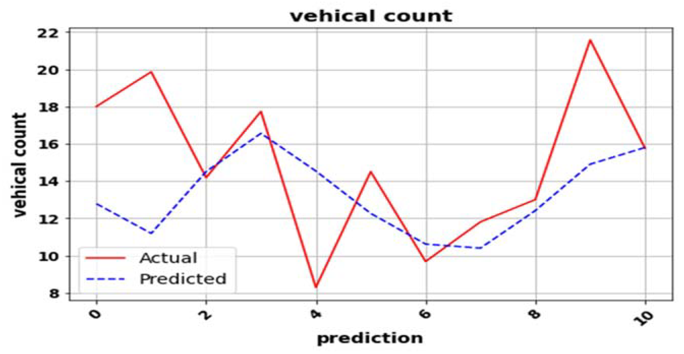
Figure 11 represents the predicted values and the actual values for the nonlinear data points using Bi-LSTM. Although losses have been reduced, the model could not achieve the actual values. Here also, one can see a vast gap between the actual and the predicted values.

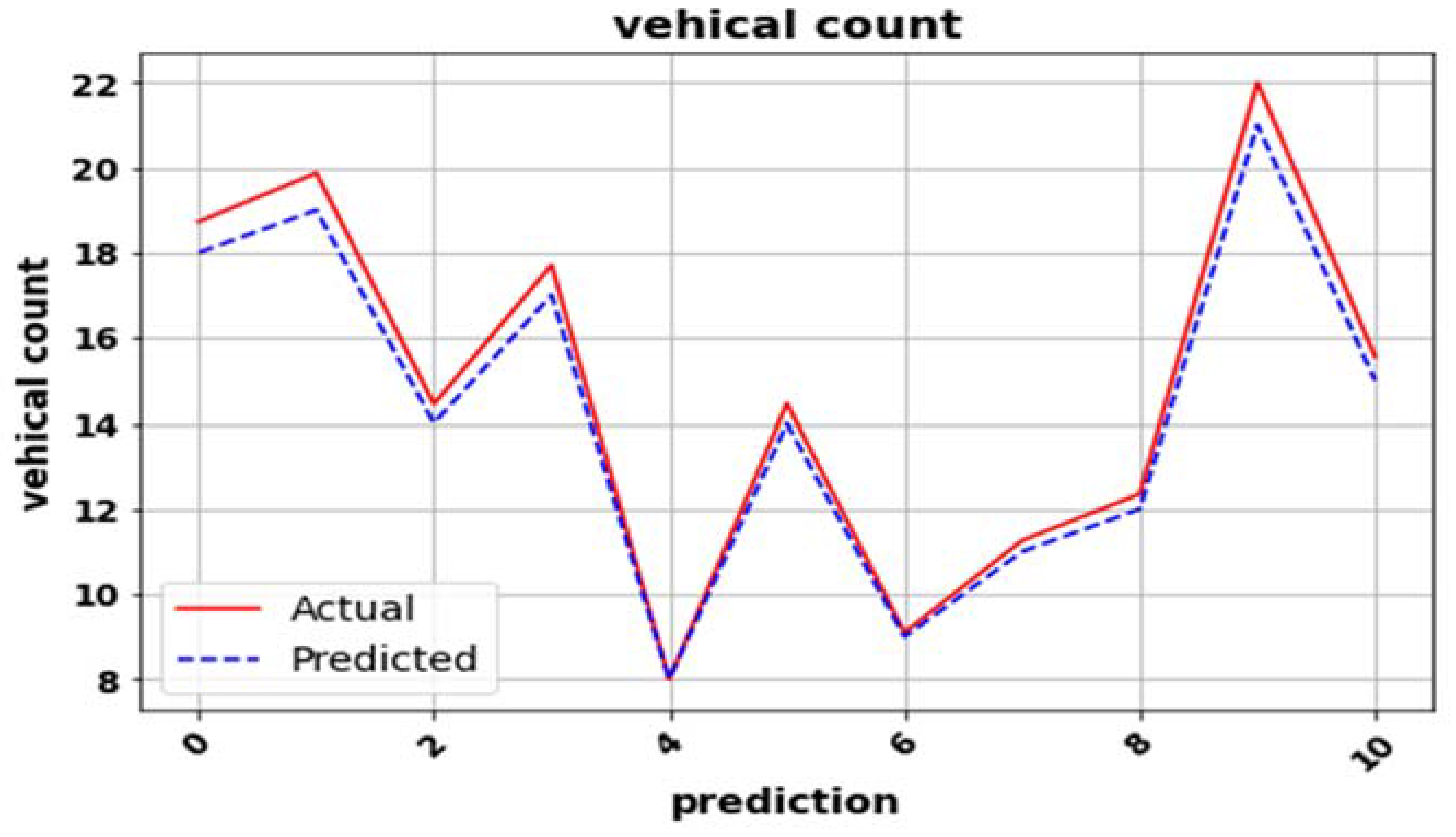
Forecast values of SARIMA and bi-LSTM are given to the back-propagation neural network (BPNN). The BPNN hybridizes the output of SARIMA and Bi-LSTM by using a nonlinear activation function that can handle both linear and nonlinear relationships among the outputs. It also optimizes the output and reduces errors by back-propagating errors in the neural network and readjusting weights again and again. Inputs given to BPNN are scaled using “Minmaxscaler()”. In total, 5000 epochs are used to reduce errors and the learning rate is taken as 0.9. Figure 12 represents the predicted and actual values of the proposed hybrid SARIMA Bi-LSTM model optimized by the BPNN model.

Table 4. Comparative analysis of models.

S. No.	Model	MSE	MAE	RMSE	MAPE
1.	Graph CNN + LSTM [13]	--	4.11	5.879	0.145
2.	ARIMA + MLP [16]	0.71	0.55	0.84	--
3.	ARIMA + RNN [16]	0.66	0.53	0.81	--
4.	ARIMA + LSTM [17]	241.66	6.53	15.54	0.119
5.	ARIMA+ LSTM + BP [35]	--	20.00	33.17	14.13
6.	ANN [36]	--	3.866	--	--
7.	SARIMA	23.36	4.06	4.63	0.388
8.	Bi-LSTM	25.62	4.2	5.06	0.31
9.	SARIMA + Bi-LSTM	17.79	3.04	4.21	0.20
10.	Proposed model (SARIMA + Bi-LSTM + BPNN)	0.337	0.499	0.58	0.03

presents the comparative analysis of existing models with the proposed model. The proposed hybrid model (SARIMA + bi-LSTM optimized with BPNN) performs best with MSE as 0.337, MAE as 0.499, RMSE as 0.58, and MAPE as 0.03 compared to standalone SARIMA, bi-LSTM models. SARIMA comes up with MSE, MAE, RMSE, and MAPE values as 23.36, 4.06, 4.63, and 0.388, respectively. Bi-LSTM gave MSE, MAE, RMSE, and MAPE as 25.62, 4.2, 5.06, and 0.31, respectively. The hybrid model (SARIMA + bi-LSTM) gave MSE, MAE, RMSE, and MAPE values as 17.79, 3.04, 4.21, and 0.20, respectively. This hybrid model is created by simply adding the linear and nonlinear forecasted values.

In addition, a similar technique is used by Y. Deng et al. [35] to predict outpatient visits to the hospital. The authors used the ARIMA model to handle linearity and the LSTM model to handle the nonlinearity of the time-series dataset. These forecasted values are optimized using back propagation. This model performs much better than its component machine learning models and produces a MAE value of 20.00, RMSE of 33.17, and MAPE of 14.13. However, our proposed approach performed much better than the model given by Y. Deng et al.

6. Conclusions

Road traffic is considered a major cause of air pollution and degradation of air quality. Reducing the traffic congestion problem helps to create a sustainable healthy environment. It also saves a lot of time for the people travelling, which indirectly helps national economic growth. A new hybridized model is proposed using SARIMA and Bi-LSTM. The proposed model has been experimented with using “CityPulse”, a smart city big IoT time-series dataset. The proposed hybrid model uses the “vehicalcount” feature of the dataset to predict traffic congestion. The SARIMA model trains the linear values of the dataset and then its residual nonlinear values are fed to the Bi-LSTM model. Predicted values of SARIAM and Bi-LSTM are combined using a BP neural network. Comparative analysis of the proposed univariate hybrid model is undertaken with existing models using MAE, MSE, RMSE, and MAPE error-measuring matrices. MAE and MSE came out to be 0.499, 0.337, 0.58, and 0.03 for the proposed hybrid univariate model.

The proposed model can be used to reduce traffic on the roads, which in turn, helps to make smart cites free of air pollution and noise pollution. The proposed model can be used for stock trend forecasting, disease prediction, weather prediction, or any kind of time-series dataset prediction problem.

The proposed model has some limitations such as only a few features being considered for evaluating the model as per the chosen dataset. Various external factors like weather, external events, peak hours, etc. can be considered in future enhancement of this work. Future work also focuses on enhancing the performance by using some interpretation analysis methods of the proposed model. Detailed interpretation analysis approaches such as LIME, SHAP, etc. help to explain the decisions or predictions provided by the proposed model.

References

1. Zheng, Z.; Yang, Y.; Liu, J.; Dai, H.-N.; Zhang, Y. Deep and Embedded Learning Approach for Traffic Flow Prediction in Urban Informatics. IEEE Trans. Intell. Transp. Syst. 2019, 20, 3927–3939. [Google Scholar] [CrossRef]
2. Kashyap, A.A.; Raviraj, S.; Devarakonda, A.; Nayak, K.S.R.; Kv, S.; Bhat, S.J. Traffic flow prediction models—A review of deep learning techniques. Cogent Eng. 2022, 9, 2010510. [Google Scholar] [CrossRef]
3. Sarrab, M.; Pulparambil, S.; Awadalla, M. Development of an IoT based real-time traffic monitoring system for city governance. Glob. Transit. 2020, 2, 230–245. [Google Scholar] [CrossRef]
4. Guerrero-Ibáñez, J.; Zeadally, S.; Contreras-Castillo, J. Sensor Technologies for Intelligent Transportation Systems. Sensors 2018, 18, 1212. [Google Scholar] [CrossRef] [PubMed]
5. Chahal, A.; Gulia, P.; Gill, N.S. Different analytical frameworks and big data model for Internet of Things. Indones. J. Electr. Eng. Comput. Sci. 2022, 25, 1159–1166. [Google Scholar] [CrossRef]
6. Yadav, S.; Gulia, P.; Gill, N.S. Flow-MotionNet: A neural network-based video compression architecture. Multimed. Tools Appl. 2022, 81, 42783–42804. [Google Scholar] [CrossRef]
7. Javaid, S.; Sufian, A.; Pervaiz, S.; Tanveer, M. Smart traffic management system using Internet of Things. In Proceedings of the International Conference on Advanced Communication Technology, ICACT, Chuncheon-si, Republic of Korea, 11–14 February 2018; pp. 393–398. [Google Scholar] [CrossRef]
8. Rejeb, A.; Rejeb, K.; Simske, S.; Treiblmaier, H.; Zailani, S. The big picture on the internet of things and the smart city: A review of what we know and what we need to know. Internet Things 2022, 19, 100565. [Google Scholar] [CrossRef]
9. Zafar, N.; Haq, I.U.; Chughtai, J.-R.; Shafiq, O. Applying Hybrid Lstm-Gru Model Based on Heterogeneous Data Sources for Traffic Speed Prediction in Urban Areas. Sensors 2022, 22, 3348. [Google Scholar] [CrossRef]
10. Sun, T.; Sun, B.; Jiang, Z.; Hao, R.; Xie, J. Traffic Flow Online Prediction Based on a Generative Adversarial Network with Multi-Source Data. Sustainability 2021, 13, 12188. [Google Scholar] [CrossRef]
11. Majumdar, S.; Subhani, M.M.; Roullier, B.; Anjum, A.; Zhu, R. Congestion prediction for smart sustainable cities using IoT and machine learning approaches. Sustain. Cities Soc. 2021, 64, 102500. [Google Scholar] [CrossRef]
12. Feng, X.; Ling, X.; Zheng, H.; Chen, Z.; Xu, Y. Adaptive Multi-Kernel SVM with Spatial–Temporal Correlation for Short-Term Traffic Flow Prediction. IEEE Trans. Intell. Transp. Syst. 2019, 20, 2001–2013. [Google Scholar] [CrossRef]
13. Bogaerts, T.; Masegosa, A.D.; Angarita-Zapata, J.S.; Onieva, E.; Hellinckx, P. A graph CNN-LSTM neural network for short and long-term traffic forecasting based on trajectory data. Transp. Res. Part C Emerg. Technol. 2020, 112, 62–77. [Google Scholar] [CrossRef]
14. Neelakandan, S.; Berlin, M.A.; Tripathi, S.; Devi, V.B.; Bhardwaj, I.; Arulkumar, N. IoT-based traffic prediction and traffic signal control system for smart city. Soft Comput. 2021, 25, 12241–12248. [Google Scholar] [CrossRef]
15. Aid, A.; Khan, M.A.; Abbas, S.; Ahmad, G.; Fatimat, A. Modelling smart road traffic congestion control system using machine learning techniques. Neural Netw. World 2019, 29, 99–110. [Google Scholar] [CrossRef]
16. Rajalakshmi, V.; Vaidyanathan, S.G. Hybrid Time-Series Forecasting Models for Traffic Flow Prediction. Promet Traffic Transp. 2022, 34, 537–549. [Google Scholar] [CrossRef]
17. Lu, S.; Zhang, Q.; Chen, G.; Seng, D. A combined method for short-term traffic flow prediction based on recurrent neural network. Alex. Eng. J. 2021, 60, 87–94. [Google Scholar] [CrossRef]
18. Tseng, F.-H.; Hsueh, J.-H.; Tseng, C.-W.; Yang, Y.-T.; Chao, H.-C.; Chou, L.-D. Congestion prediction with big data for real-time highway traffic. IEEE Access 2018, 6, 57311–57323. [Google Scholar] [CrossRef]
19. Yi, H.; Jung, H.; Bae, S. Deep Neural Networks for traffic flow prediction. In Proceedings of the 2017 IEEE International Conference on Big Data and Smart Computing (BigComp), Jeju, Republic of Korea, 13–16 February 2017; pp. 328–331. [Google Scholar] [CrossRef]
20. Bernaś, M. WSN Power Conservation Using Mobile Sink for Road Traffic Monitoring. In Computer Networks, Communications in Computer and Information Science; Kwiecień, A., Gaj, P., Stera, P., Eds.; Springer: Berlin/Heidelberg, Germany, 2013; pp. 476–484. [Google Scholar] [CrossRef]
21. Bernaś, M. VANETs as a Part of Weather Warning Systems. In Computer Networks, Communications in Computer and Information Science; Kwiecień, A., Gaj, P., Stera, P., Eds.; Springer: Berlin/Heidelberg, Germany, 2012; pp. 459–466. [Google Scholar] [CrossRef]
22. Bernas, M.; Płaczek, B.; Korski, W. Wireless Network with Bluetooth Low Energy Beacons for Vehicle Detection and Classification. In Computer Networks, Communications in Computer and Information Science; Gaj, P., Sawicki, M., Suchacka, G., Kwiecień, A., Eds.; Springer International Publishing: Cham, Switzerland, 2018; pp. 429–444. [Google Scholar] [CrossRef]
23. Zahid, M.; Chen, Y.; Jamal, A.; Mamadou, C.Z. Freeway Short-Term Travel Speed Prediction Based on Data Collection Time-Horizons: A Fast Forest Quantile Regression Approach. Sustainability 2020, 12, 646. [Google Scholar] [CrossRef]
24. Zahid, M.; Chen, Y.; Jamal, A.; Memon, M.Q. Short Term Traffic State Prediction via Hyperparameter Optimization Based Classifiers. Sensors 2020, 20, 685. [Google Scholar] [CrossRef]
25. Chaturvedi, S.; Rajasekar, E.; Natarajan, S.; McCullen, N. A comparative assessment of SARIMA, LSTM RNN and Fb Prophet models to forecast total and peak monthly energy demand for India. Energy Policy 2022, 168, 113097. [Google Scholar] [CrossRef]
26. Medina-Salgado, B.; Sánchez-DelaCruz, E.; Pozos-Parra, P.; Sierra, J.E. Urban traffic flow prediction techniques: A review. Sustain. Comput. Inform. Syst. 2022, 35, 100739. [Google Scholar] [CrossRef]
27. Muneer, A.; Ali, R.F.; Almaghthawi, A.; Taib, S.M.; Alghamdi, A.; Ghaleb, E.A.A. Short term residential load forecasting using long short-term memory recurrent neural network. Int. J. Electr. Comput. Eng. 2022, 12, 5589–5599. [Google Scholar] [CrossRef]
28. Li, Y.-H.; Harfiya, L.N.; Purwandari, K.; Lin, Y.-D. Real-Time Cuffless Continuous Blood Pressure Estimation Using Deep Learning Model. Sensors 2020, 20, 5606. [Google Scholar] [CrossRef]
29. Wang, L.; Xu, X.; Su, Q.; Song, Y.; Wang, H.; Xie, M. Automatic gear shift strategy for manual transmission of mine truck based on Bi-LSTM network. Expert Syst. Appl. 2022, 209, 118197. [Google Scholar] [CrossRef]
30. Cai, L.; Zhou, S.; Yan, X.; Yuan, R. A Stacked BiLSTM Neural Network Based on Coattention Mechanism for Question Answering. Comput. Intell. Neurosci. 2019, 2019, e9543490. [Google Scholar] [CrossRef]
31. Sun, W.; Wang, Y. Short-term wind speed forecasting based on fast ensemble empirical mode decomposition, phase space reconstruction, sample entropy and improved back-propagation neural network. Energy Convers. Manag. 2018, 157, 1–12. [Google Scholar] [CrossRef]
32. Ali, M.I.; Gao, F.; Mileo, A. CityBench: A Configurable Benchmark to Evaluate RSP Engines Using Smart City Datasets. In Proceedings of the Semantic Web—ISWC 2015—14th International Semantic Web Conference, Bethlehem, PA, USA, 11–15 October 2015. [Google Scholar]
33. Tönjes, R.; Barnaghi, P.; Ali, M.; Mileo, A.; Hauswirth, M.; Ganz, F.; Ganea, S.; Kjærgaard, B.; Kuemper, D.; Nechifor, S.; et al. Vestergaard. Real Time IoT Stream Processing and Large-scale Data Analytics for Smart City Applications. In Poster Session, European Conference on Networks and Communications; University of Surrey: Surrey, England, 2014. [Google Scholar]
34. Kingma, D.P.; Ba, J. Adam: A method for stochastic optimization. arXiv 2014, arXiv:1412.6980. [Google Scholar]
35. Deng, Y.; Fan, H.; Wu, S. A hybrid ARIMA-LSTM model optimized by BP in the forecast of outpatient visits. J. Ambient Intell. Human Comput. 2020, in press. [Google Scholar] [CrossRef]
36. He, J.; Bai, J. Prediction Technology for Parking Occupancy Based on Multi-dimensional Spatial-Temporal Causality and ANN Algorithm. In Green, Pervasive, and Cloud Computing: 15th International Conference, GPC 2020, Xi’an, China, 13–15 November 2020, Proceedings 15; Lecture Notes in Computer Science (including subseries Lecture Notes in Artificial Intelligence and Lecture Notes in Bioinformatics) 12398 LNCS; Springer: Berlin/Heidelberg, Germany, 2020; pp. 244–256. [Google Scholar] [CrossRef]
Figure 1. Smart traffic monitoring communication system [3].
Information 14 00268 g001
Figure 2. LSTM model.
Information 14 00268 g002
Figure 3. Bi-LSTM model architecture.
Information 14 00268 g003
Figure 4. Algorithm of error back-propagation.
Information 14 00268 g004
Figure 5. Proposed SARIMA Bi-LSTM model optimized by BPNN.
Information 14 00268 g005
Figure 6. Decomposition of the dataset.
Information 14 00268 g006
Figure 7. Diagnosis of SARIMA model.
Information 14 00268 g007
Figure 8. Forecast vs. actual values of SARIMA model.
Information 14 00268 g008
Figure 9. Residual values of SARIMA model.
Information 14 00268 g009
Figure 10. Training vs. validation dataset losses.
Information 14 00268 g010
Figure 11. Actual vs. predicted values of hybrid ARIMA–Bi-LSTM model.
Information 14 00268 g011
Figure 12. Actual vs. predicted values of proposed model.
Information 14 00268 g012