Article

Towards Fault Tolerance of Reservoir Computing in Time Series Prediction

1
College of Artificial Intelligence, North China University of Science and Technology, Bohai Road, Tangshan 063210, China
2
Hebei Key Laboratory of Industrial Perception, Tangshan 063210, China
*
Author to whom correspondence should be addressed.
Information 2023, 14(5), 266; https://doi.org/10.3390/info14050266
Submission received: 4 April 2023 / Revised: 21 April 2023 / Accepted: 27 April 2023 / Published: 30 April 2023

Abstract

:
During the deployment of practical applications, reservoir computing (RC) is highly susceptible to radiation effects, temperature changes, and other factors. Normal reservoirs are difficult to vouch for. To solve this problem, this paper proposed a random adaptive fault tolerance mechanism for an echo state network, i.e., RAFT-ESN, to handle the crash or Byzantine faults of reservoir neurons. In our consideration, the faulty neurons were automatically detected and located based on the abnormalities of reservoir state output. The synapses connected to them were adaptively disconnected and withdrawn from the current computational task. On the widely used time series with different sources and features, the experimental results show that our proposal can achieve an effective performance recovery in the case of reservoir neuron faults, including prediction accuracy and short-term memory capacity (MC). Additionally, its utility was validated by statistical distributions.

1. Introduction

As a back propagation-decorrelation learning rule in machine learning, RC has emerged as a promising method for designing and training recurrent neural networks (RNN) [1]. The echo state network (ESN), proposed by Herbert Jaeger, is the most representative model in RC [2]. Its key part is a well-known reservoir structure with a great many neurons that plays the role of information transformation, in which there exist sparse random connections or self-connections that are the main method of information transfer between neurons. Only the output weights need to be solved during training, which can be achieved by a simple linear regression method. In particular, input weights and internal weights are randomly generated and kept constant during the ESN training process. Additionally, ESN possesses an impressive echo state property (ESP), when its spectral radius λ is appropriately configured, i.e.,  0 < λ < 1 . Given these, ESN can effectively overcome the disadvantages of traditional RNN training, which is prone to the disappearance and the explosion of the gradient. It has been widely applied in various fields, such as time series prediction [3,4], audio classification [5], fault diagnosis [6], language modeling [7], resource management [8], and target tracking [9].
Currently, reservoir adaptation has always been an intractable problem in ESN modeling. A great many studies focus on structure design [3,10], parameter optimization [11,12], and interpretability [13,14]. For the above ESN paradigms, there is a popular supposition that, as typical artificial neural networks, they possess some attractive inherent behavioral features of biological systems, namely the tolerance against inaccuracy, indeterminacy, and faults [15]. However, in practical application, the fault tolerance of ESNs is generally ignored. In this case, ESNs without built-in or proven fault tolerance can cause catastrophic network failures due to errors in critical components. There are many causes of ESN unreliability, especially in safety-critical applications, such as complex and harsh environments (atmospheric radiation, radioactive impurities), temperature variations, voltage instability, wear, and aging of the underlying semiconductor devices and hardware devices [16,17], which can lead to the failure of the internal neurons of the reservoir at the software level, i.e., software failure, affecting the normal computation of the ESN.
From this, it can be seen that fault tolerance should actually be a vital component of the research on RC adaptability issues, which to some extent directly determines the ability of reservoirs to be applied to practical problems. Unfortunately, the study of the fault-tolerance problem in the RC framework has not been carried out yet. To this end, an efficient fault-tolerant design is urgently needed to ensure that RC continues to operate normally in the presence of faults.

1.1. Related Work

Research related to fault tolerance theory includes both passive and active fault tolerance processing, and most of the methods are focused on feed-forward neural networks. For example, in passive methods, adding redundancy, improving learning or training algorithms, and network optimization under constraints can improve the inherent fault tolerance of neural networks. Increased redundancy refers to the duplication of key neurons and the unnecessary removal of synaptic weights. The main purpose of the improved learning/training algorithm is to change the traditional neural network training/learning model oriented to a posteriori fault tolerance, i.e., to complete the corresponding computational tasks with explicit fault tolerance goals while training/learning. The constrained neural network optimization approach is to transform the learning process and fault tolerance into a nonlinear optimization problem to find a more optimal network structure and its parameter configuration to ensure the task processing in fault mode. The related work is shown in Table 1. As can be seen from the table, in essence, passive fault-tolerant technology has no fault diagnosis, relearning, or reconfiguration process to determine the exact location of the fault, but only uses the inherent redundancy of the neural network to cover up the impact of the fault, but these faults still exist.
In the active approach, low-latency fault detection and recovery techniques allow neural networks to recover from faults. The related work is shown in Table 2.
It can be seen that the active fault-tolerant method gives timely compensation through adaptive, retraining, or self-healing mechanisms, which will be an effective processing technique for the study of fault tolerance in neural networks.
Although a significant amount of fruitful work has been carried out on the problem of fault tolerance in neural networks, most of the research has focused on feed-forward neural networks, and fault tolerance research on such feedback-type neural networks, such as reservoir computation, has not yet been addressed. In contrast, the application of feedback-type neural networks has more obvious advantages in terms of computational convergence speed, associative memory, and optimal computation. In view of this, this paper intended to carry out the study of fault tolerance methods in the framework of reservoir computing and explore the fault tolerance of reservoirs by using active fault tolerance methods from the perspective of random faults of neurons, which is a new attempt and has important value and significance for improving the theory of neural networks and exploring the application potential of reservoir computing.

1.2. Contributions

In this article, we proposed an active fault-tolerant mechanism to reconfigure the ESN model, called RAFT-ESN, for time series prediction. The main goal of the proposed approach was to make the ESN adaptively tolerate the occurrence of random faults in the neurons and recover from them to maintain the normal operation. The main contributions of this paper are summarized in Table 3.
The rest of this paper is structured as follows. Section 2 introduces the fault-tolerant ESN structure and the fault-handling process. Section 3 gives the experimental simulation for the fault-tolerant theoretical scheme proposed in this paper. Finally, Section 4 gives the conclusion.
In addition, we provide the list of notation descriptions used to construct the fault-tolerant model for Section 2, as shown in Table 4.

2. Fault Tolerant Echo State Networks

2.1. Model Structure

Generally, reservoir neurons easily yield random faults, as described in the introduction section. To solve this problem, we developed a fault-tolerant echo state network (RAFT-ESN), as shown in Figure 1.
Structurally, it is similar to the traditional ESN, including an input layer, a reservoir layer, and a linear readout layer. However, the key difference is that our proposal can adaptively tackle the faulty neurons in this reservoir (marked in red), which terminate the computation (failure/crash), or send outliers (Byzantine failure). The state update of RAFT-ESN is performed by the following transition function:
x ( t + 1 ) = f ( W i n u ( t + 1 ) + W x ( t ) + W b a c k y ( t ) ) ,
where f ( · ) is the activation function of the reservoir neuron, generally t a n h . The final model readout is calculated as follows:
y ( t + 1 ) = W o u t x ( t + 1 ) .
Similarly, the training aim of our RAFT-ESN is to discover the optimal W o u t . It is a linear regression problem, solved by the Moore–Penrose pseudo-inversion in our scenario, given by
W o u t = X ˜ Y = ( X T X ) 1 X T Y .

2.2. Random Fault Tolerance Mechanism

The aim of this paper was to endow the ESN with the special property that the projection capability of the reservoir remains available even if some neurons become abnormal. We designed a simple, straightforward, and effective processing mechanism that adaptively counteracts the faults once the neurons in the reservoir fail. Firstly, we give the behavior criterion of the faulty neuron as follows:
  • If the state output value of the neuron inside the reservoir is in the range of (−1, 1), then it is not at fault;
  • If the state output value of the neuron inside the reservoir is always stuck at 0, it experiences a computational crash;
  • If the state output value of the neuron inside the reservoir is always stuck at ± 1 or arbitrarily deviates from the expected value, a Byzantine fault occurs [15].
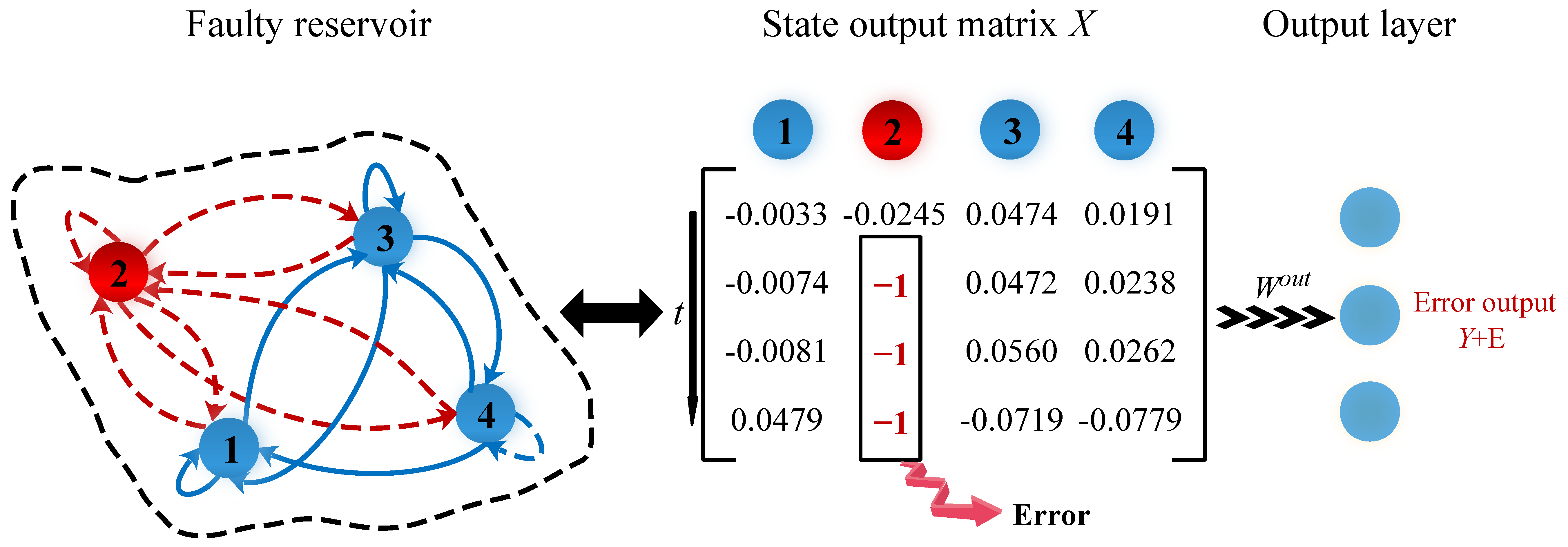
According to the above criterion, when a neuron is faulty, its corresponding state output is suddenly stuck at −1, marked by red in Figure 2. In this case, the synapses connected to the faulty neuron cannot transmit information properly and, therefore, the final network output deviates from its expected value, i.e.,  Y + E .
For the given faulty reservoir, to ensure that it can function properly, the fault detection mechanism is first used to detect and locate the faulty neurons. Then, the synapses connected to them are disconnected according to a fault tolerance strategy to make these faulty neurons withdraw from the current computational task; this fault tolerance rule is given by
W N × N W ( N N f a i l ) × ( N N f a i l ) W i n N × K W i n ( N N f a i l ) × K W b a c k N × L W b a c k ( N N f a i l ) × L W o u t L × N W o u t L × ( N N f a i l ) ,
where N f a i l denotes the number of faulty reservoir neurons. As seen in Equation (4), the  N f a i l neurons associated with the input, reservoir, and output layers are disconnected from each other. Subsequently, the model is retrained to achieve fault tolerance so that it can be used for continuous prediction tasks.

2.3. Fault Handling Process

Algorithm 1 gives the random fault handling process for neurons. It contains the initialization of the model, the training process, fault detection, fault tolerance processing, and the retraining process. Among them, Algorithm 2 is invoked for detecting faulty neurons, and Algorithm 3 is called for fault-tolerant processing. In our scheme, the neuron for random faults is characterized by a state output value that always remains at −1. In this way, our proposed model can continuously detect faults during operation and automatically adapt to the needs of different prediction tasks.
Here, the main algorithmic process is executed first, i.e., the execution of Algorithm 1. In Algorithm 1, the  input is the hyperparameters of the reservoir and the output is the trained optimal solution W o u t . First, the ESN is initialized and configured. After that, the training process of the model is started and Algorithm 2 is called to determine whether the ESN is faulty or not. If there is a fault after detection, we will invoke the Algorithm 3 to repair the model, i.e., fault tolerance for reservoir neuron faults. Here, we added the training process and the self-detection mechanism to the whole loop function, one after another, to prevent the reservoir neuron from failing again after the training was completed. Specifically, the loop continuously determines whether the trained reservoir neuron is faulty and, if it is faulty after training, it starts to repair until no fault occurs after training, and the whole loop is terminated. At this point, the whole ESN training process will also be completed.
Algorithm 1 Random fault processing on neurons.
1:
Input: Sample data u ( t ) , y ( t ) , reservoir size N, spectral radius λ , state collection time T and washing time T 0
2:
Output: Output weight matrix W o u t
3:
♯ Initialize ESN
4:
Randomly generate W i n , W, W b a c k
5:
Set λ ( 0 , 1 )
6:
Configure an ESN
7:
while true do
8:
    ♯ Training ESN
9:
    for t = T 0 to T do
10:
        Update reservoir states using Equation (1)
11:
        Collect network state X and output Y
12:
    end for
13:
    Solve W o u t using Equation (3)
14:
    ♯ Self-testing of reservoir neuron faults after training
15:
    if Fault Detection then
16:
        Fault Tolerance Method
17:
    else
18:
        break
19:
    end if
20:
end while
For Algorithm 2, the core idea is to determine whether a neuron has a problem by detecting whether the state output value of each neuron in the reservoir is −1. Specifically, first, the input parameter of the algorithm is the reservoir state X, and the number of neurons N is obtained from X. After that, the state output value of each neuron is detected in turn in a loop, and when the presence of a neuron with an output value of −1 is detected, the error message is returned to Algorithm 1.
Algorithm 2 Fault detection method.
1:
Input: Network state X
2:
Output: flag
3:
Get reservoir size N from X
4:
fori = 1 to N do
5:
    if find(X(:, i) = −1) != null then
6:
        return true
7:
    else
8:
        return false
9:
    end if
10:
end for
Algorithm 3 Fault tolerance method.
1:
Input: Faulty ESN, Network state X
2:
Output: Normal ESN
3:
Get W from Faulty ESN
4:
Get reservoir size N from Faulty ESN
5:
♯ Locating faults
6:
Define an array eNode
7:
fori = 1 to N do
8:
    if find(X(:, i) = −1) != null then
9:
        add i to eNode
10:
    end if
11:
end for
12:
fors = 1 to size eNode do
13:
    k = eNode(s)
14:
    ♯ Remove the faulty reservoir neurons guaranteeing the normal ESN operation;
15:
    W(k,:)=[ ] and W(:,k)=[ ]
16:
end for
17:
Update N, W i n , W b a c k and W o u t using Equation (4)
For Algorithm 3, the input parameters include the faulty ESN model and its network state X, and the output is the normal ESN model. First, the internal weights W and reservoir size N are obtained from the ESN. Second, a detection mechanism is used to locate the faulty neuron and the fault tolerance is applied to the faulty neuron after the location is completed. In the fault-tolerant mechanism, the faulty neurons are sequentially acquired and made to exit the current repository computation task. Meanwhile, all neurons in the input, repository, and output layers are automatically disconnected from these faulty neurons. Then, the new N, W i n , W b a c k and W o u t are obtained using the formula (4), and the fault-tolerant ESN model is returned to Algorithm 1.

3. Simulation Experiments

In this section, we performed a comprehensive experimental evaluation of the RAFT-ESN model, considering the following prediction tasks, such as the Henon map system, the nonlinear autoregressive moving average (NARMA) system, the multiple superposition oscillator (MSO) problem, and cellular network traffic data (cars, pedestrians, trains). Such heterogeneous and different types of time series data can provide strong data support to verify the validity and reliability of the fault tolerance model. In particular, all our experimental results were obtained by averaging after five experiments, and the fault-tolerant recoverability performance of the model was verified from the perspective of recovery performance, short-term memory capacity (MC), and statistical analysis.

3.1. Datasets and Experimental Settings

(1) Henon map: The Henon map is a classical discrete-time dynamical system that can generate chaotic phenomena and becomes a simplified method with which to study the dynamics of Lorentzian systems [28]. The Henon map chaotic time series is simply constructed by the following equation:
h ( t ) = 1 1.4 h ( t 1 ) 2 + 0.3 h ( t 2 ) + τ ( t ) ,
where h ( t ) is the system output at time t and τ ( t ) is the Gaussian white noise with a standard deviation of 0.0025. We used the sequence length of L = 3000 .
(2) NARMA systerm:The NARMA system is a highly chaotic discrete-time system that has become a widely-studied benchmark problem [4]. The current output depends on the input and the previous output, and the non-correlation between the inputs may lead to difficulties in pattern learning. This NARMA system is defined as follows:
y ( t + 1 ) = a 1 y ( t ) + a 2 y ( t ) i = 1 k y ( t i ) + a 3 n ( t ( k 1 ) ) n ( t ) + a 4 ,
where n ( t ) is the input to the system at time t, and k is the system order, generally k = 10 , characterizing the long-range dependence between data, and a 1 = 0.3 , a 2 = 0.05 , a 3 = 1.5 , and a 4 = 0.1 . This dataset was normalized and rescaled in [0, 1] and its length was L = 3000 .
(3) MSO problem:The MSO time series, as a benchmark problem, was used to assess the recoverability of the RAFT-ESN model. The MSO time series data were generated by summing several simple sinusoidal functions of different frequencies [29], given by
y ( u ) = i = 1 n sin ( α i u ) ,
where n denotes the number of sinusoidal functions, generally k = 7, u is the integer subscript of the time step, α i is the corresponding frequency, having α 1 = 0.2 , α 2 = 0.311 , α 3 = 0.42 , α 4 = 0.51 , α 5 = 0.63 , α 6 = 0.74 , α 7 = 0.85 . α 5 = 0.63 , α 6 = 0.74 , and α 7 = 0.85 . In experiments, the MSO time series with the length of 3000 was considered for prediction.
(4) Cellular network traffic prediction:This 4G cellular network traffic dataset was supplied by the Irish mobile operator. The dataset contains client cellular key performance indicators for different mobility modes such as cars, pedestrians and trains [30]. The sampling interval for each mobile dataset was one sample per second, with a monitoring duration of roughly 15 min and a visual throughput of between 0 and 173 Mbit/s. Each mobile mode dataset contains channel quality, context-dependent metrics, downlink and uplink throughputs, and cell-related information. In our consideration, the downlink throughputs of the car, pedestrian, and train mobility modes were chosen to verify the performance of our proposal with data lengths of 2992, 1540, and 1410, respectively.
In fact, our considered mobile traffic traces from a real cellular network had significant burstiness, chaos, periodicity, and a large number of missing values. Therefore, pre-processing the data helps the model to make accurate predictions. To ensure accurate prediction, the interpolation method was used to fill in missing data with previous data, and Gaussian smoothing was used to mitigate the effects of fluctuations and outliers, providing an effective trade-off between data characteristics and nonlinear approximation performance.
In our experiments, a 1-100-1 model structure was used for the first three-time series and a 1-50-1 model structure was used for the last class of data, and the other parameters were set as shown in Table 5. In particular, the faults of the reservoir neurons were generated randomly.

3.2. Evaluation Metrics

To evaluate the recoverable performance of our model, three metrics such as normalized root mean square error (NRMSE), mean absolute error (MAE), and coefficient of determination (R 2 ) were considered as follows:
N R M S E = t = 1 L ( Y t r u ( t ) Y p r e ( t ) ) 2 L σ p r e 2 M A E = 1 L t = 1 L | Y p r e ( t ) Y t r u ( t ) | R 2 = 1 t = 1 L ( Y p r e ( t ) Y t r u ( i ) ) 2 t = 1 L ( Y t r u ( t ) Y ¯ ) 2 ,
where L is the length of the time series, Y t r u (t) and Y p r e (t) are the actual and predicted values at the time step t, respectively, Y ¯ represents the mean of actual time series, and σ p r e 2 is the variance of predicted values.

3.3. Recoverable Performance Analysis

Table 6 shows the results of the tolerance performance evaluation of RAFT-ESN in six time series prediction tasks, where WESN is a well-functioning ESN. It can be seen from the table that, according to the above three performance metrics, the prediction accuracy of our proposed RAFT-ESN is close to that of WESN in the Henon map prediction task, while achieving a better prediction performance in the remaining prediction tasks. This indicates that the reservoir can be recovered from the failure using our adaptive fault tolerance method. The recovered RAFT-ESN achieves a better prediction performance because of its inherently redundant topology, and our scheme precisely removes the redundant faulty nodes and reassigns the computational tasks to good neurons through retraining, and the reservoir still maintains a good mapping capability for different prediction tasks. These features enable RAFT-ESN to recover adaptively to a better prediction performance after a failure, thus ensuring validity and reliability.
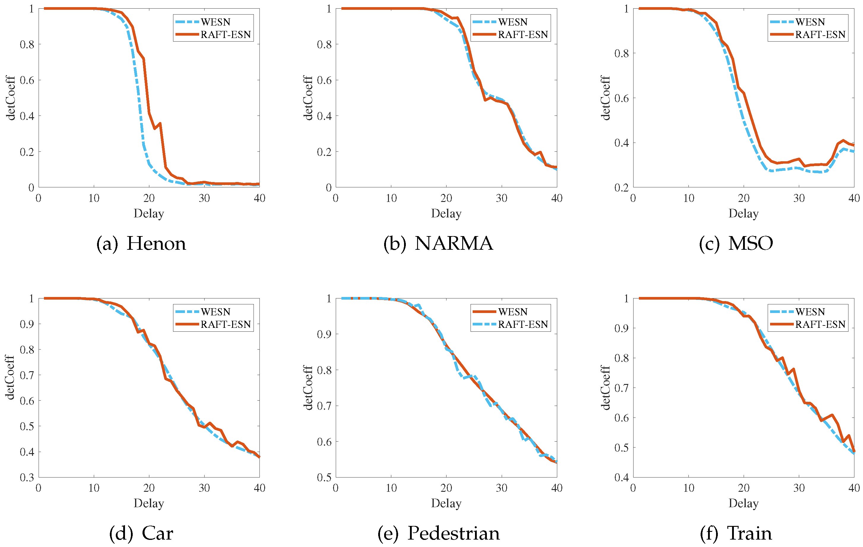
In addition, memory capacity (MC) was employed to assess the fault tolerance of reservoir neurons [15]. Here, we investigated the temporal processing capacity of our RAFT-ESN by means of short-time memory (STM). In general, STM allows the input signal to be reconstructed from a previous time t; in other words, how much historical information can be recorded in the instantaneous response of the system [31]. In the STM evaluation we considered, the initial ESN network, equipped with one input node, 50 linear reservoir nodes and one output node, was trained to remember input delays of k = 1 , 2 , , 40 . Meanwhile, we considered the following reservoir configuration, whose spectral radius and sparsity were set to 0.8 and 0.1, respectively.
Figure 3 gives the memory decay curves of RAFT-ESN for six time series prediction tasks, indicating the degree of recovery of 40 reservoir neurons for one input, where detCoeff is the squared correlation coefficient, i.e., MC. If MC is superimposed, it represents the STM of the reservoir. In all prediction tasks, RAFT-ESN can approximate the recovery to the initial memory capacity. Further quantitative results are shown in Table 7. The approximate STM between RAFT-ESN and WESN in these prediction tasks means the achievable fault-tolerant capacity.

3.4. Statistical Validation

In this section, we illustrate the validity of the recoverable performance of the proposed model in terms of statistical validation, such as scatter plot with edge density profile, violin plot, and T-test.
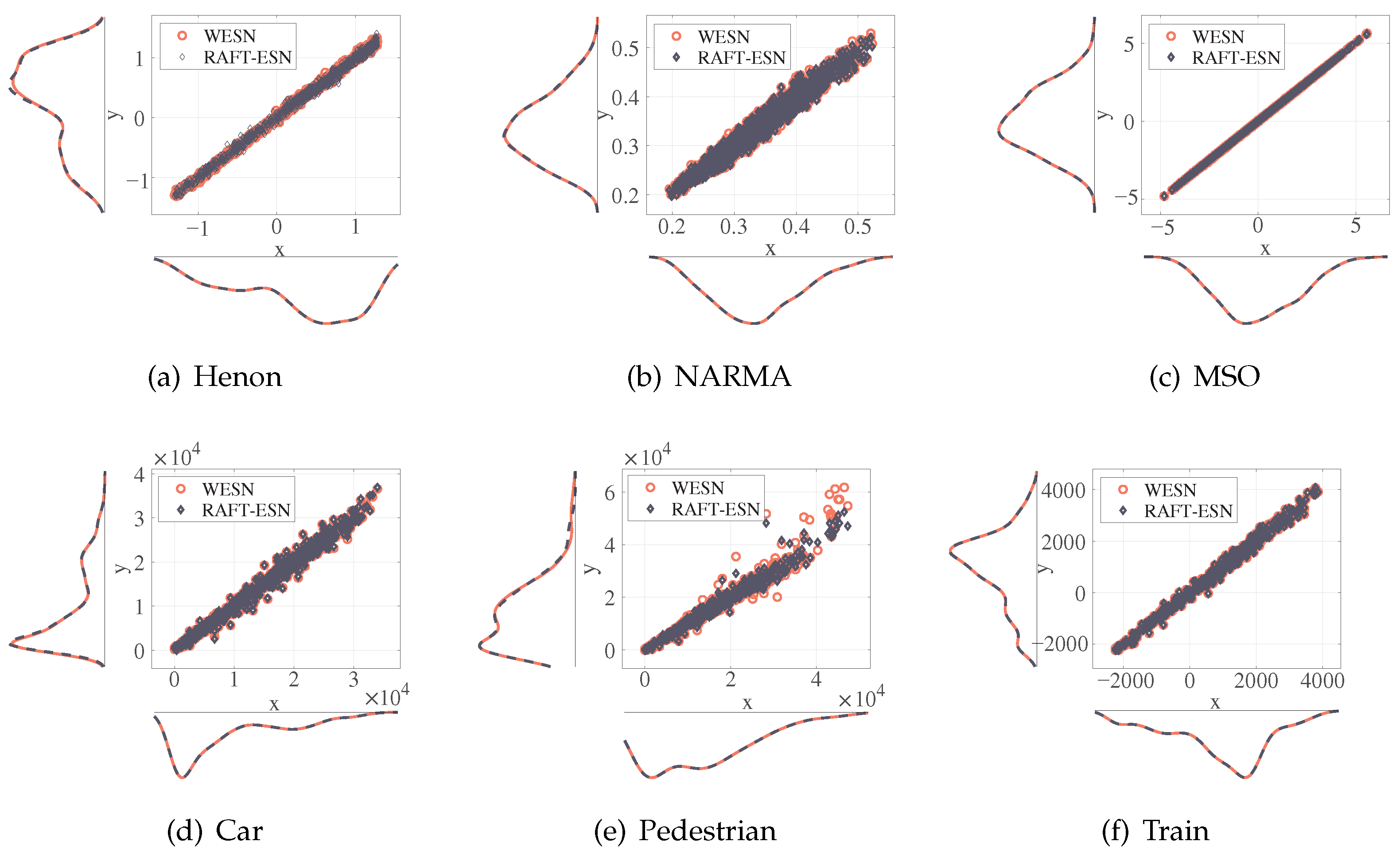
Figure 4 presents violin plots for the real data and predicted data of RAFT-ESN and WESN on all-time series prediction tasks, where each consists of a box plot and density traces located on its left and right sides. From this figure, we can see that our proposed RAFT-ESN has similar density distribution statistics and box plots to the predicted output of WESN, indicating the similarity in prediction performance and the fault-tolerant model that has been repaired from faults in both. It is worth noting that, although the predicted values of the fault-tolerant model deviate slightly from those of the original model in some scenarios, as in Figure 4e, this only slightly affects the fault-tolerance capability of RAFT-ESN. Further, by observing Figure 5, we find that the data distributions of the two models are also similar. The combined violin plots and scatter plots with edge density curves visualize that RAFT-ESN has a similar predictive performance to WESN from the perspective of statistical distribution, which implies that our proposed model can recover well under failure modes through the fault tolerance mechanism.
Finally, the T-test was used to verify the validity of the recovery performance of RAFT-ESN, and the test results are shown in Table 8. In the table, the H values of the fault-tolerant model are all zero, implying that its predicted and true values are data belonging to the same distribution. In the first three prediction tasks, the P values of the fault-tolerant model and the original model are close to each other and are all higher than 0.05, indicating that the differences between the predicted and true values of the two are not significant. It is worth noting that, in the actual network traffic prediction tasks, the variability between the predicted values of the fault-tolerant model and true values is smaller, indicating that the prediction results of the model are more realistic and reliable. In summary, the effectiveness of the recoverable performance of RAFT-ESN is further verified based on the T test analysis.

4. Conclusions

In this work, a RAFT-ESN model that can adaptively tolerate neuron failures was proposed to maintain the normal operation of the reservoir and to ensure its effectiveness and reliability during practical deployment, thus enhancing the value of practical applications. We investigated the failure modes of reservoir neurons. Based on this, a fault detection mechanism was designed to determine the broken-down neurons. We developed a fault-tolerant strategy that can automatically disconnect the synaptic connections between faulty neurons and their associated neurons, allowing the RC to adaptively offset the faults to maintain normal and efficient prediction. Through a large number of different kinds of time series prediction experiments, we verified that RAFT-ESN has an excellent recovery performance for abnormal or crashed faults of reservoir neurons. In the future, we can try to extend the fault tolerance strategy to synaptic faults and even solve more complex problems, such as cases in which neuron faults coexist with synaptic faults, in order to obtain more robust and reliable RCs in practical applications.

Author Contributions

Conceptualization, X.S.; Software, J.G.; Formal analysis, Y.W.; Visualization, J.G.; Investigation, X.S.; Methodology, X.S. and J.G.; Validation, X.S. and J.G.; Writing—Original draft, J.G.; Writing—Review & editing, J.G. All authors have read and agreed to the published version of the manuscript.

Funding

This work was supported in part by the Science and Technology Project of Hebei Education Department, Grant ZD2021088, and in part by the open fund project from Marine Ecological Restoration and Smart Ocean Engineering Research Center of Hebei Province, Grant HBMESO2315.

Institutional Review Board Statement

Not applicable.

Informed Consent Statement

Not applicable.

Data Availability Statement

The datasets for this study are available upon request from the corresponding author.

Acknowledgments

We would like to thank Yingqi Li for her contribution to funding acquisition and other aspects, as well as Xin Feng and his related units for their technical and financial support, and the editorial board and all reviewers for their professional suggestions to improve this paper.

Conflicts of Interest

The authors declare no conflict of interest.

References

  1. Vlachasa, P.R.; Pathakbc, J.; Huntde, B.R.; Sapsisf, T.P.; Girvan, M.; Ott, E.; Koumoutsakosa, P. Backpropagation algorithms and reservoir computing in recurrent neural networks for the forecasting of complex spatiotemporal dynamics. Neural Netw. 2020, 126, 191–217. [Google Scholar] [CrossRef] [PubMed] [Green Version]
  2. Mansoor, M.; Grimaccia, F.; Leva, S.; Mussetta, M. Comparison of echo state network and feed-forward neural networks in electrical load forecasting for demand response programs. Math. Comput. Simul. 2021, 184, 282–293. [Google Scholar] [CrossRef]
  3. Sun, X.C.; Gui, G.; Li, Y.Q.; Liu, R.P.; An, Y.L. ResInNet: A Novel Deep Neural Network With Feature Reuse for Internet of Things. IEEE Internet Things J. 2019, 6, 679–691. [Google Scholar] [CrossRef]
  4. Sun, X.C.; Li, T.; Li, Q.; Huang, Y.; Li, Y.Q. Deep Belief Echo-State Network and Its Application to Time Series Prediction. Knowl.-Based Syst. 2017, 130, 17–29. [Google Scholar] [CrossRef]
  5. Scardapane, S.; Uncini, A. Semi-Supervised echo state networks for audio classification. Cogn. Comput. 2017, 9, 125–135. [Google Scholar] [CrossRef]
  6. Zhang, S.H.; Sun, Z.Z.; Wang, M.; Long, J.Y.; Bai, Y.; Li, C. Deep Fuzzy Echo State Networks for Machinery Fault Diagnosis. IEEE Trans. Fuzzy Syst. 2019, 28, 1205–1218. [Google Scholar] [CrossRef]
  7. Deng, H.L.; Zhang, L.; Shu, X. Feature Memory-Based Deep Recurrent Neural Network for Language Modeling. Appl. Soft Comput. 2018, 68, 432–446. [Google Scholar] [CrossRef]
  8. Chen, M.Z.; Saad, W.; Yin, C.C.; Debbah, M. Data Correlation-Aware Resource Management in Wireless Virtual Reality (VR): An Echo State Transfer Learning Approach. IEEE Trans. Commun. 2019, 67, 4267–4280. [Google Scholar] [CrossRef] [Green Version]
  9. Yang, X.F.; Zhao, F. Echo State Network and Echo State Gaussian Process for Non-Line-of-Sight Target Tracking. IEEE Syst. J. 2020, 14, 3885–3892. [Google Scholar] [CrossRef]
  10. Hu, R.; Tang, Z.R.; Song, X.; Luo, J.; Wu, E.Q.; Chang, S. Ensemble echo network with deep architecture for time-series modeling. Neural Comput. Appl. 2021, 33, 4997–5010. [Google Scholar] [CrossRef]
  11. Liu, J.X.; Sun, T.N.; Luo, Y.L.; Yang, S.; Cao, Y.; Zhai, J. Echo State Network Optimization Using Binary Grey Wolf Algorithm. Neurocomputing 2020, 385, 310–318. [Google Scholar] [CrossRef]
  12. Li, Y.; Li, F.J. PSO-based growing echo state network. Appl. Soft Comput. 2019, 85, 105774. [Google Scholar] [CrossRef]
  13. Han, X.Y.; Zhao, Y. Reservoir computing dissection and visualization based on directed network embedding. Neurocomputing 2021, 445, 134–148. [Google Scholar] [CrossRef]
  14. Barredo Arrieta, A.; Gil-Lopez, S.; Laña, I.; Bilbao, M.N.; Del Ser, J. On the post-hoc explainability of deep echo state networks for time series forecasting, image and video classification. Neural Comput. Appl. 2022, 34, 10257–10277. [Google Scholar] [CrossRef]
  15. Torres-Huitzil, C.; Girau, B. Fault and Error Tolerance in Neural Networks: A Review. IEEE Access 2017, 5, 17322–17341. [Google Scholar] [CrossRef]
  16. Li, W.S.; Ning, X.F.; Ge, G.J.; Chen, X.M.; Wang, Y.; Yang, H.Z. FTT-NAS: Discovering fault-tolerant neural architecture. In Proceedings of the 2020 25th Asia and South Pacific Design Automation Conference (ASP-DAC), Beijing, China, 13–16 January 2020; pp. 211–216. [Google Scholar] [CrossRef] [Green Version]
  17. Zhao, K.; Di, S.; Li, S.H.; Liang, X.; Zhai, Y.J.; Chen, J.Y.; Ouyang, K.M.; Cappello, F.; Chen, Z.Z. FT-CNN: Algorithm-based fault tolerance for convolutional neural networks. IEEE Trans. Parallel Distrib. Syst. 2020, 32, 1677–1689. [Google Scholar] [CrossRef]
  18. Wang, J.; Chang, Q.Q.; Chang, Q.; Liu, Y.S.; Pal, N.R. Weight noise injection-based MLPs with group lasso penalty: Asymptotic convergence and application to node pruning. IEEE Trans. Cybern. 2018, 49, 4346–4364. [Google Scholar] [CrossRef]
  19. Dey, P.; Nag, K.; Pal, T.; Pal, N.R. Regularizing multilayer perceptron for robustness. IEEE Trans. Syst. Man. Cybern. Syst. 2017, 48, 1255–1266. [Google Scholar] [CrossRef]
  20. Wang, H.; Feng, R.B.; Han, Z.F.; Leung, C.S. ADMM-based algorithm for training fault tolerant RBF networks and selecting centers. IEEE Trans. Neural Netw. Learn. Syst. 2017, 29, 3870–3878. [Google Scholar] [CrossRef]
  21. Duddu, V.; Rajesh Pillai, N.; Rao, D.V.; Balas, V.E. Fault tolerance of neural networks in adversarial settings. J. Intell. Fuzzy Syst. 2020, 38, 5897–5907. [Google Scholar] [CrossRef] [Green Version]
  22. Kosaian, J.; Rashmi, K.V. Arithmetic-intensity-guided fault tolerance for neural network inference on GPUs. In Proceedings of the International Conference for High Performance Computing, Networking, Storage and Analysis, St. Louis, MO, USA, 14–19 November 2021; pp. 1–15. [Google Scholar] [CrossRef]
  23. Gong, J.; Yang, M.F. Evolutionary fault tolerance method based on virtual reconfigurable circuit with neural network architecture. IEEE Trans. Evol. Comput. 2017, 22, 949–960. [Google Scholar] [CrossRef]
  24. Naeem, M.; McDaid, L.J.; Harkin, J.; Wade, J.J.; Marsland, J. On the role of astroglial syncytia in self-repairing spiking neural networks. IEEE Trans. Neural Netw. Learn. Syst. 2015, 26, 2370–2380. [Google Scholar] [CrossRef] [PubMed]
  25. Liu, J.X.; McDaid, L.J.; Harkin, J.; Karim, S.; Johnson, A.P.; Millard, A.G.; Hilder, J.; Halliday, D.M.; Tyrrell, A.M.; Timmis, J. Exploring self-repair in a coupled spiking astrocyte neural network. IEEE Trans. Neural Netw. Learn. Syst. 2018, 30, 865–875. [Google Scholar] [CrossRef] [PubMed] [Green Version]
  26. Liu, S.S.; Reviriego, P.; Lombardi, F. Selective neuron re-computation (SNRC) for error-tolerant neural networks. IEEE Trans. Comput. 2021, 71, 684–695. [Google Scholar] [CrossRef]
  27. Hoang, L.H.; Hanif, M.A.; Shafique, M. Ft-Clipact: Resilience Analysis of Deep Neural Networks and Improving Their Fault Tolerance Ssing Clipped Activation. In Proceedings of the 2020 Design, Automation and Test in Europe Conference and Exhibition (DATE), Grenoble, France, 9–13 March 2020; pp. 1241–1246. [Google Scholar] [CrossRef]
  28. Peng, Y.X.; Sun, K.H.; He, S.B. A discrete memristor model and its application in Hénon map. Chaos Solitons Fractals 2020, 137, 109873. [Google Scholar] [CrossRef]
  29. Li, Y.; Li, F.J. Growing deep echo state network with supervised learning for time series prediction. Appl. Soft Comput. 2022, 128, 109454. [Google Scholar] [CrossRef]
  30. Raca, D.; Quinlan, J.J.; Zahran, A.H.; Sreenan, C.J. Beyond throughput: A 4G LTE dataset with channel and context metrics. In Proceedings of the 9th ACM Multimedia Systems Conference, Amsterdam, The Netherlands, 12–15 June 2018; pp. 460–465. [Google Scholar] [CrossRef]
  31. Jaeger, H. Short Term Memory in Echo State Networks; Fraunhofer-Gesellschaft: Sankt Augustin, Germany, 2002. [Google Scholar] [CrossRef]
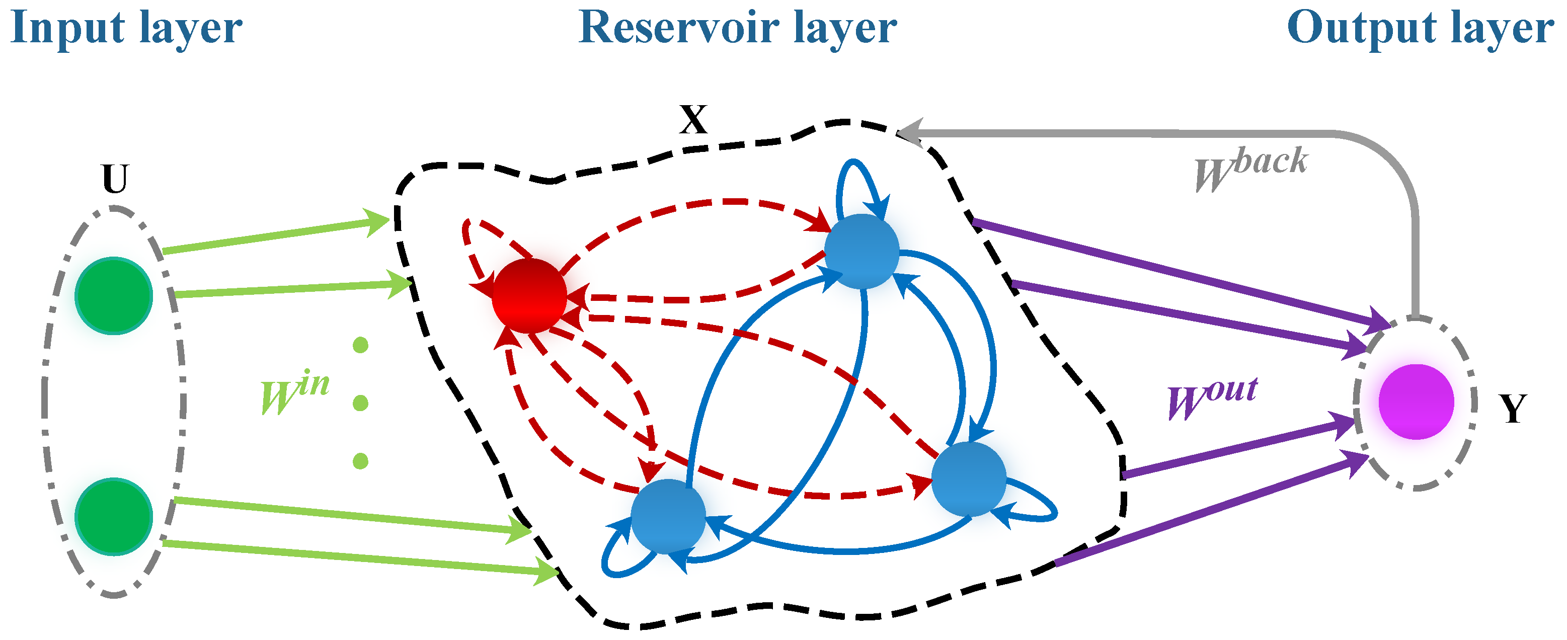
Figure 1. Schematic representation of our RAFT-ESN.
Information 14 00266 g001
Figure 2. Errorsin reservoir neurons computations.
Information 14 00266 g002
Figure 3. Forgetting curves of RAFT-ESN in six time series prediction tasks.
Information 14 00266 g003
Figure 4. Violin plots of RAFT-ESN prediction outputs in six time series prediction tasks.
Information 14 00266 g004
Figure 5. Scatter plot of the edge density curve for the predicted output of RAFT-ESN in six time series prediction tasks.
Information 14 00266 g005
Table 1. Research on fault-tolerance of neural networks based on passive methods.
Fault TypeFault Tolerance MethodMain IdeaLiterature
Number
Neuron faultsRedundancy
removed
Remove redundant nodes in hidden layer based on Lasso penalty term[18]
Weight perturbationImproved
algorithm
Introduce three regularization terms to penalize the systematic error[19]
Weight perturbationImproved
algorithm
Fault tolerance objective function with l 1 -parametric term[20]
External interferenceImproved
training
Train deep neural network (DNN) with input noise and gradient noise[21]
Convolutional layer faultImproved
algorithm
Based on four algorithm-based fault tolerance (ABFT) schemes[17]
Neural network layersImproved
algorithm
Strength-guided ABFT reduces the time of redundant fault-tolerant execution of neural networks[22]
Neuron removalGenetic
algorithm
Genetic algorithm-based fault tolerance using programmable structures[23]
Table 2. Research on fault-tolerance of neural networks based on active methods.
Fault TypeFault Tolerance MethodMain IdeaLiterature Number
Neuron failureRecovery techniqueReestablishing neuronal firing activity by enhancing the weight of healthy synapses[24]
Weight failureRecovery techniqueMapping between input and output is established by Bienenstock Cooper Munro learning rules[25]
Neuron faultsRecovery techniqueRecalculate those neurons with unreliable classification results[26]
Weight perturbationLow-latency fault detectionUsing error mitigation techniques to improve DNN failure recovery capability[27]
Table 3. Summary of the main contributions of this paper.
Serial
Number
Contributions
1We constructed ESN models with random neuron failures based on the original ESN, considering and analyzing the behavioral pattern of reservoir neurons with random failures during network training.
2For random faults of neurons, we proposed a fault detection mechanism to detect whether faults occur during network training.
3We designed an active fault tolerance strategy to adaptively withdraw the randomly faulty neurons from the current computational task and maintain the normal operation of RC.
4We gave the main algorithm flows of the proposed model, including the neuron random fault handling algorithm, the fault detection algorithm, and the random fault tolerance algorithm.
5We evaluated the proposed model using a number of widely-used time series benchmarks with different sources and characteristics, experimentally verifying the effectiveness of the fault tolerance scheme and that the proposed model is able to recover from faults.
Table 4. List of notations used to build the fault-tolerant model.
VariablesMeaning
Random variables
KThe size of the ESN input layer is K
NThe size of the reservoir neuron is N
LThe size of the ESN output layer is L
EThe output error of the reservoir is E
Matrix variables
u ( t ) K Network input at time t
x ( t ) N The state output of the reservoir neuron at time t
y ( t ) L The L-dimensional readout at time t
W i n N × K The input weight matrix from K input to N reservoir neurons
W N × N The internal weight matrix of N reservoir neurons
W b a c k N × L The feedback weight matrix from L readout neuron to N reservoir neurons
W o u t L × N The output weight matrix of the ESN network
XReservoir state collection matrix
X ˜ Generalized inverse matrix of X
YTarget output matrix of ESN network
Table 5. Model hyperparameter settings.
ParameterSize
Spectral radius0.8
Reservoir sparsity0.1
Dataset division1:1
Maximum ratio of neural faults10%
Table 6. Tolerance performance evaluation of RAFT-ESN in six time series prediction tasks.
DataModelNRMSEMAER 2
Henon MapRAFT-ESN0.07040.00500.9949
WESN0.04860.00240.9976
NARMARAFT-ESN0.20230.04090.9590
WESN0.20730.04300.9570
MSORAFT-ESN0.00775.9671 × 10 5 0.9999
WESN0.01271.6164 × 10 4 0.9998
CarRAFT-ESN0.09210.00850.9915
WESN0.09540.00910.9909
PedestrianRAFT-ESN0.21970.04830.9516
WESN0.14710.02160.9783
TrainRAFT-ESN0.09880.00980.9902
WESN0.10030.01010.9899
Table 7. STM capability of RAFT-ESN in six prediction tasks.
ModleHenon MapNARMAMSOCarPedestrianTrain
RAFT-ESN19.827929.055425.578129.055433.063933.8662
WESN17.973228.886124.306228.886133.113033.8940
Table 8. T-test of RAFT-ESN in six time series prediction tasks.
DataParametersRAFT-ESNWESN
Henon MapH00
p0.98680.9734
NARMAH00
p0.80240.7401
MSOH00
p0.99740.9885
CarH00
p0.62210.7520
PedestrianH00
p0.64710.7974
TrainH00
p0.94130.9488
Disclaimer/Publisher’s Note: The statements, opinions and data contained in all publications are solely those of the individual author(s) and contributor(s) and not of MDPI and/or the editor(s). MDPI and/or the editor(s) disclaim responsibility for any injury to people or property resulting from any ideas, methods, instructions or products referred to in the content.