Energy Usage Forecasting Model Based on Long Short-Term Memory (LSTM) and eXplainable Artificial Intelligence (XAI)

Abstract

The accurate forecasting of energy consumption is essential for companies, primarily for planning energy procurement. An overestimated or underestimated forecasting value may lead to inefficient energy usage. Inefficient energy usage could also lead to financial consequences for the company, since it will generate a high cost of energy production. Therefore, in this study, we proposed an energy usage forecasting model and parameter analysis using long short-term memory (LSTM) and explainable artificial intelligence (XAI), respectively. A public energy usage dataset from a steel company was used in this study to evaluate our models and compare them with previous study results. The results showed that our models achieved the lowest root mean squared error (RMSE) scores by up to 0.08, 0.07, and 0.07 for the single-layer LSTM, double-layer LSTM, and bi-directional LSTM, respectively. In addition, the interpretability analysis using XAI revealed that two parameters, namely the leading current reactive power and the number of seconds from midnight, had a strong influence on the model output. Finally, it is expected that our study could be useful for industry practitioners, providing LSTM models for accurate energy forecasting and offering insight for policymakers and industry leaders so that they can make more informed decisions about resource allocation and investment, develop more effective strategies for reducing energy consumption, and support the transition toward sustainable development.

1. Introduction

Energy consumption has been rapidly increasing in recent years in line with the advancement of the industrial sector. The development of industry has also mirrored the rise in populations and economic growth all around the globe. Hence, energy is considered one of the main factors of national development and plays a significant part in the national policy of many countries [1]. Nevertheless, the energy sector is currently facing several challenges, including the need to reduce greenhouse gas emissions, increase energy security, and promote economic growth. To address these challenges, the International Energy Agency (IEA) has recommended a range of measures, including the development of more advanced energy usage forecasting models [2]. These models can help to support the transition towards a more sustainable energy sector by providing insight into future energy demand, the potential impacts of policy decisions, and the feasibility of different energy technologies [3].

An accurate forecasting model of energy usage can provide a useful guide for planning and distribution. Therefore, various approaches to energy forecasting have been proposed, including the use of statistical methods, machine learning algorithms, and physics-based models. The earliest approach utilized statistical methods, which were primarily applied in the past to forecast energy demand. For instance, Kandananond [4] utilized a variety of methods, including autoregressive integrated moving average (ARIMA) and multiple linear regression (MLR), to forecast energy consumption. Another statistical model based on the underlying physical concepts was proposed as a method for estimating energy consumption in [5]. Due to the unusual patterns of energy demand, linear statistical techniques have only a limited ability to capture nonlinearity in energy consumption factors [6]. ML has been widely adopted for prediction tasks in various domains, including healthcare [7], disease prevention [8], environmental science [9], and the energy sector itself [10,11]. In the industry sector, the use of ML is even more extensive for early fault detection and the condition monitoring of industrial equipment [12,13,14,15]. These studies showed that such techniques could improve equipment reliability, reduce downtime and maintenance costs, and increase operational efficiency. The methods used included dynamic identification; on-device intelligence; and deep-learning-based approaches, such as convolutional neural networks and long short-term memory models. These studies highlighted the potential of using advanced analytics and artificial intelligence in industrial applications to improve equipment performance and reduce downtime.

Due to their potential to extract representative features from historical data, ML-based models have delivered more promising results than physical and statistical methods [16]. Support vector machine (SVM), gradient boosting system (GBM), random forest (RF), and artificial neural networks (ANNs) are the most prevalent machine learning algorithms utilized in business to estimate energy consumption [17]. Typically, these models are utilized to manage the nonlinear interactions between input and output data. Within AI ML approaches, artificial neural network (ANN) models have produced favorable outcomes for real-time predictions, particularly when learning from dynamic changes in environmental variables becomes a critical factor for prediction accuracy [18].

The use of deep neural networks (DNNs) or deep learning (DL) is the most recent development in ANN-based energy forecasting models to be discussed in the energy forecasting literature [19,20]. The number of hidden layers in a neural network may be increased via deep learning techniques, which are also particularly effective at handling data with significant nonlinear properties [21]. To predict energy consumption, DL-based models have also been investigated, and these techniques have shown superior performance when compared to other models. For instance, Wang et al. [22] constructed a model based on a CNN and generative adversarial networks for the categorization of the weather and yielded significant improvements compared to the previous model using regular ANNs. In addition to this, Zang et al. [23] created CNN-based models to predict solar electricity and determine the day-to-day electricity price.

In the case of energy forecasting, a recurrent neural network (RNN) is a DNN-based architecture that is better-suited for time-series data, since it is meant to extract temporal information from data [24]. RNNs can maintain temporal information by introducing the notion of a recurrent layer to determine whether to preserve knowledge from prior instances [25]. Due to the exploding/vanishing gradient issue, RNNs are unable to sustain long-term reliance effectively. According to a recent study [26], RNNs are also not appropriate for large-displacement-value predictions in the slope-sliding process. To overcome these issues, LSTM networks were proposed [27] as enhanced RNNs. By including gate architectures and memory cells, LSTM solves the exploding/vanishing gradient issue and preserves temporal correlation [28]. In the energy forecasting problem, an experiment with an LSTM model for power output forecasting had superior performance compared to a CNN-based model [29,30].

Even though DL-based approaches have yielded excellent forecasting accuracy, it is difficult to describe how they arrived at their conclusions [31,32]. Researchers have referred to these methodologies as “black box” models as a direct result of this effect. In recent years, the subject of explainable artificial intelligence (XAI), which has become one of the most prominent research fields, has attracted the attention of several academics. This is because the goal of XAI is to design machine learning models with the capacity to be explained. Over the past decade, the field of XAI has grown dramatically [33,34]. This has led to the creation of a multitude of domain-dependent and context-specific methods for interpreting ML models and creating explanations that can be understood by non-experts in this domain [35,36].

This study aimed to contribute to the field of energy usage forecasting by introducing a novel approach that combines LSTM models with XAI. While LSTM models have been widely used for time-series forecasting, the inclusion of XAI techniques provided a unique way to understand and interpret the model’s decision-making process, which could enhance the transparency of and trust in the model’s predictions. By combining these two approaches, the proposed model could provide more accurate energy usage forecasts while also offering insights into the factors that contributed to these forecasts, which could be particularly useful for energy management and planning purposes. Overall, this paper’s contribution is to propose a more accurate, interpretable, and practical approach to energy usage forecasting, which could have significant implications for energy efficiency and sustainability.

2. Materials and Methods

Figure 1 shows the general flow/framework of the study. In the beginning, the energy dataset was used to form the forecasting model. Several steps were required, such as data pre-processing, data splitting for training and validation, model building and selections, and performance metric measurements. Finally, XAI was applied to analyze the most influential features for forecasting model performance.

2.1. Dataset Description and Data Preprocessing

In this work, data on energy consumption were used for the construction of the forecasting models. The information was obtained from the DAEWOO steel company in Gwangyang City, which is located in South Korea. This company creates many different types of coils, as well as steel sheets and iron plates. The information regarding the amount of energy used can be found on the website of the Korea Electric Power Corporation at https://pccs.kepco.go.kr (accessed on 10 October 2022). Information such as the amount of electricity used, the lagging and leading current reactive power, the lagging and leading current power factor, the carbon dioxide (tCO₂) emissions, and the types of loads is included in the data that are maintained on the website.

Table 1. Dataset properties of energy usage considered in our study.

Variable	Data Type	Measure
Industry energy consumption	Continuous	kWh
Lagging current reactive power	Continuous	kVarh
Leading current reactive power	Continuous	kVarh
tCO2 (CO2)	Continuous	Ppm
Lagging current power factor	Continuous	%
Leading current power factor	Continuous	%
Number of seconds from midnight (NSM)	Continuous	Seconds
Week status	Categorical	Weekday, weekend
Load type	Categorical	Light, medium, maximum

presents an overview of each attribute contained within the dataset. Regarding the variables mentioned in Table 1, week status is a categorical variable that by default was unsuitable for LSTM. Nevertheless, instead of deliberately removing this variable, we transformed it into an ordinal variable by attaching a value of 0 to weekends and 1 to weekdays. The value of weekdays was higher than that of weekends because, according to the dataset, the electrical load during weekdays was always higher than on weekends. Another categorical variable was load type. Nevertheless, since load type is an ordinal categorical variable, we could simply attribute values of 1, 2, and 3 to light, medium, and maximum loads, respectively.

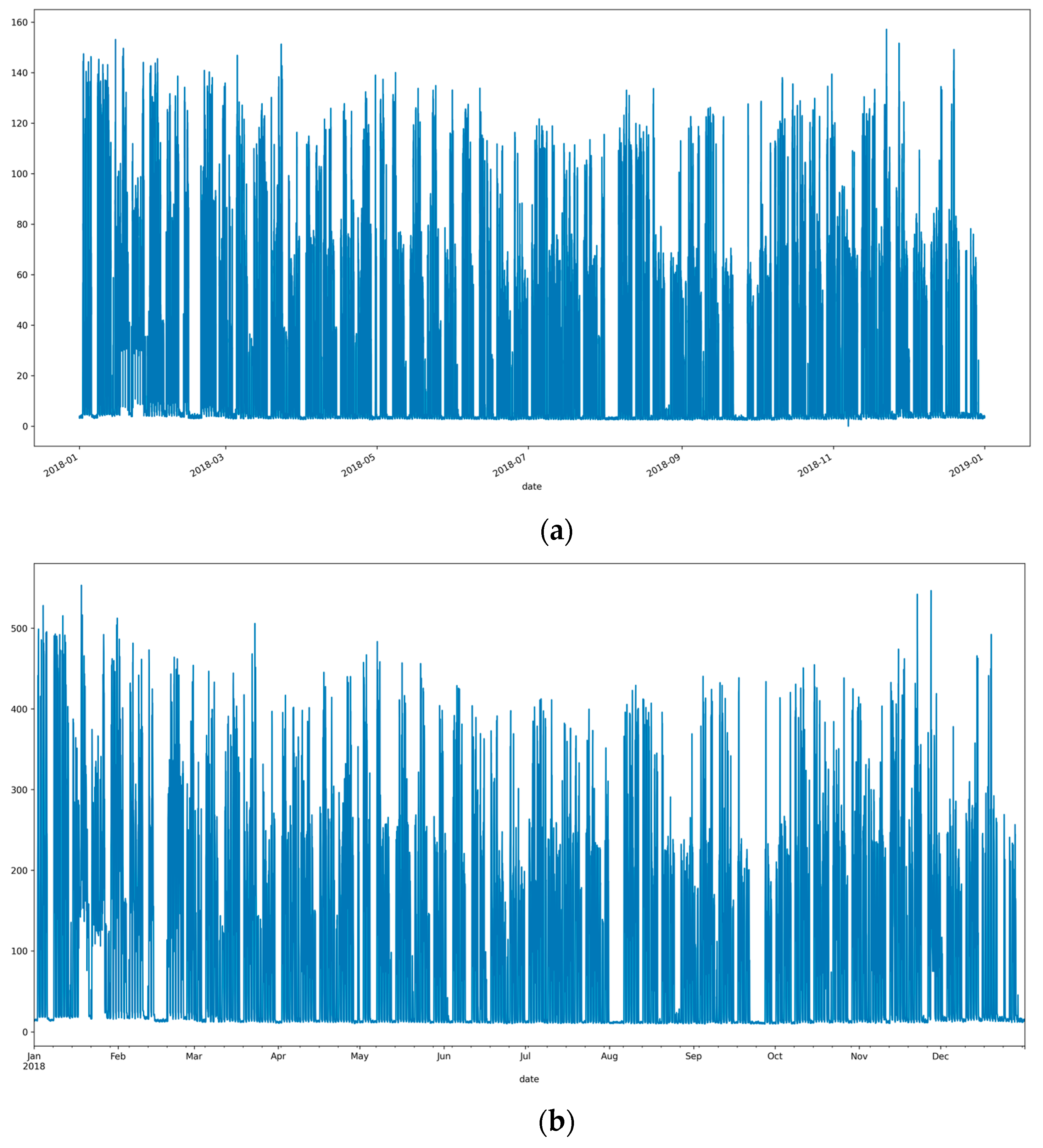
The data outlined in Table 1 were recorded for the company every 15 min for a period of 365 days (2018, 12 months). To build the forecasting model, we smoothed the data with downsampling techniques and transformed the energy usage data to 1 h intervals using suitable aggregate functions for each column/variable. Figure 2a,b show visual representations of the energy usage at 15 min and 1 h intervals, respectively.

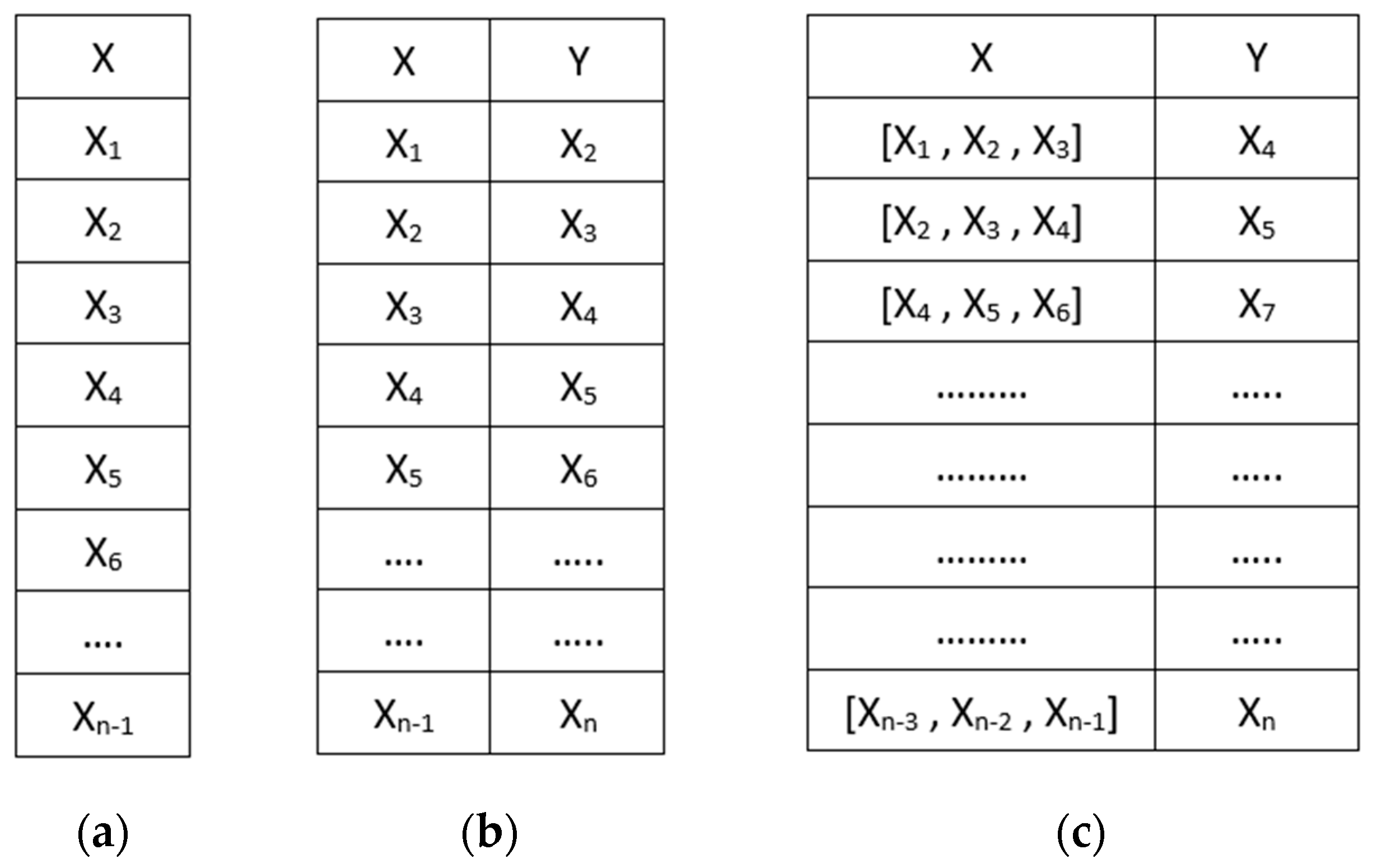
The dataset then needed to be prepared to make it suitable for time-series forecasting. For time-series forecasting, the dataset was then transformed into a sub-sequential form using sliding-window techniques. In general, sliding-window techniques take the last n datapoints from a dataset to predict the data in the n + 1 positions. Figure 3 illustrates the dataset transformation with 1 window (see Figure 3b) and 3 windows (see Figure 3c) from the original dataset (see Figure 3a).

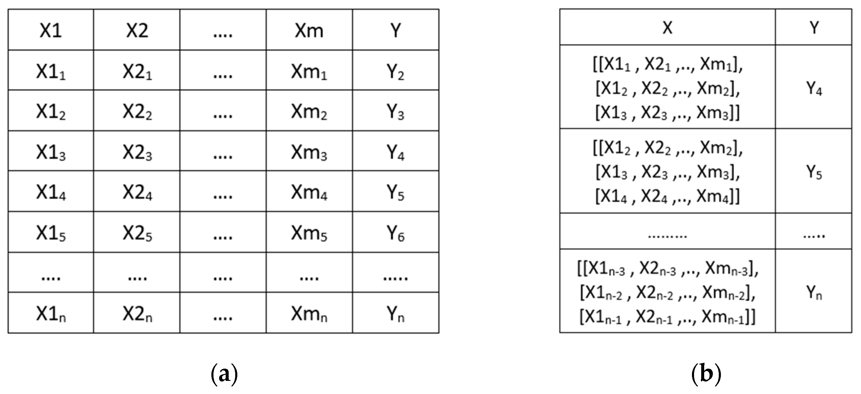
Because the dataset utilized in this experiment consisted of more than one attribute, the issue could be understood as a multivariate problem. In the case of a multivariate input, a problem may have two or more concurrent input time series in addition to an output time series that is dependent on the input time series. Because each series had observations at the same time steps, the input for the multivariate time series was carried out in a parallel fashion. The illustration in Figure 4 provides a better understanding of the data transformation of the multivariate time-series inputs, showing the data representation containing n attributes. The original form of the data is illustrated in Figure 4a, and the data formatted with 3 sliding windows are shown in Figure 4b. In the data table in Figure 4, X1_t, X2_t, …, Xm_t are the multivariate attributes, while (x − 1)_t−1, (x − 1)_t−2, …, (X − 1)_t−n represent the values of x for the previous n time sequences.

2.2. Long Short-Term Memory

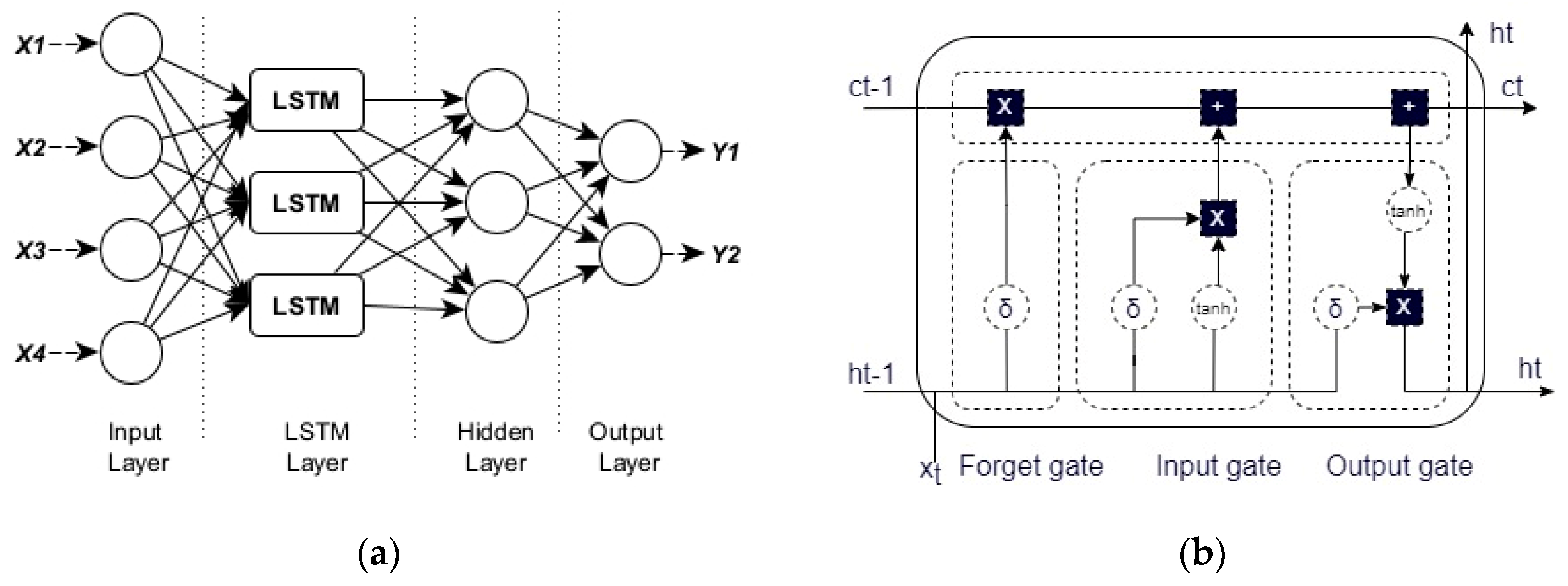
LSTM is a subset of recurrent neural networks designed to process time-series data [27]. Long short-term memory is a mechanism derived from RNNs. LSTM is highly effective in solving sequence forecasting problems because it can store historical data using the standard recurrent layer, self-loops, and the internal unique gate structure. Thus, the LSTM network efficiently addresses the forgetting and gradient vanishing issues of typical RNNs [37]. In addition, LSTM may be trained to achieve multi-step forecasting, which is important for predicting time series [38]. Figure 5a illustrates the architecture of an LSTM network. The LSTM network has a hidden layer consisting of a set of LSTM cells. Figure 5b illustrates the structure of an LSTM cell. Four gates comprise an LSTM neural network unit: an input gate, a cell state, a forgetting gate, and an output gate, as illustrated in Figure 5b. The forgetting gate is used to identify which messages pass through the cell and enter the input gate, which determines the number of new messages to add to the cell’s state; subsequently, it decides the output message via the output gate [39]. In Figure 5b, $f_t,i_t,o_t,c_t$, and $h_t$ denote the output of the forgetting gate, the input gate, the output gate, the memory unit, and the hidden unit, respectively, at time $t$.

As shown in Figure 5, the process of inputting data in the LSTM architecture begins at the forgetting gate, which is responsible for determining which information from the memory unit state $c_{t-1}$ should be forgotten or maintained in the current memory unit state $c_t$. The forgetting gate’s output ranges from 0 to 1. When the output is closer to zero, it is necessary to forget more past information, and vice versa.

The output of the forgetting gate was calculated using Formula (1). In Formulas (1) and (2), $W$ and $U$ indicate the weight matrix concerning the input and hidden units, respectively. In addition, $b$ denotes the bias matrix, whereas $⨂$ represents the element-by-element multiplication of two vectors. The initial value is specified as $c_0=h_0=0$.

$${\mathrm{f}}_{\mathrm{t}}=\mathsf{\sigma }(W_f{x}_t+U_f{h}_t-1+b_f)$$

(1)

Afterward, the process moves to the input gate. The purpose of the input gate is to determine which information from an input $x_t$ must be updated in the current state of the memory unit $c_t$. The output of the input gate was calculated by Formula (2), below.

$$\begin{gathered} {\mathrm{i}}_{\mathrm{t}}=\mathsf{\sigma }\left(W_i{x}_t+U_i{h}_t-1+b_i\right), \\ {\tilde{\mathrm{c}}}_{\mathrm{t}}=\mathrm{t}\mathrm{a}\mathrm{n}\mathrm{h}\left(W_c{x}_t+U_c{h}_t-1+b_c\right) \end{gathered}$$

(2)

During the process within the input gate, a portion of the information in the memory unit $c_{t-1}$ is discarded, and a portion of the vital information in $x_t$ is transferred to the memory unit $c_t$. The process of updating the information was performed using the following Formula (3).

$${\mathrm{c}}_{\mathrm{t}}=f_t⨂c_t+i_t⨂{\tilde{c}}_t$$

(3)

Finally, the last calculation was performed on the output gate, which is responsible for determining which information from the current memory unit $c_t$ must be transmitted to the current hidden unit ${\mathrm{h}}_{\mathrm{t}}$. The value of the current hidden unit was then calculated with Formula (4).

$${\mathrm{h}}_{\mathrm{t}}=\mathsf{\sigma }\left(W_o{x}_t+U_o{h}_t-1+b_o\right)⨂\mathrm{t}\mathrm{a}\mathrm{n}\mathrm{h}\left(c_t\right)$$

(4)

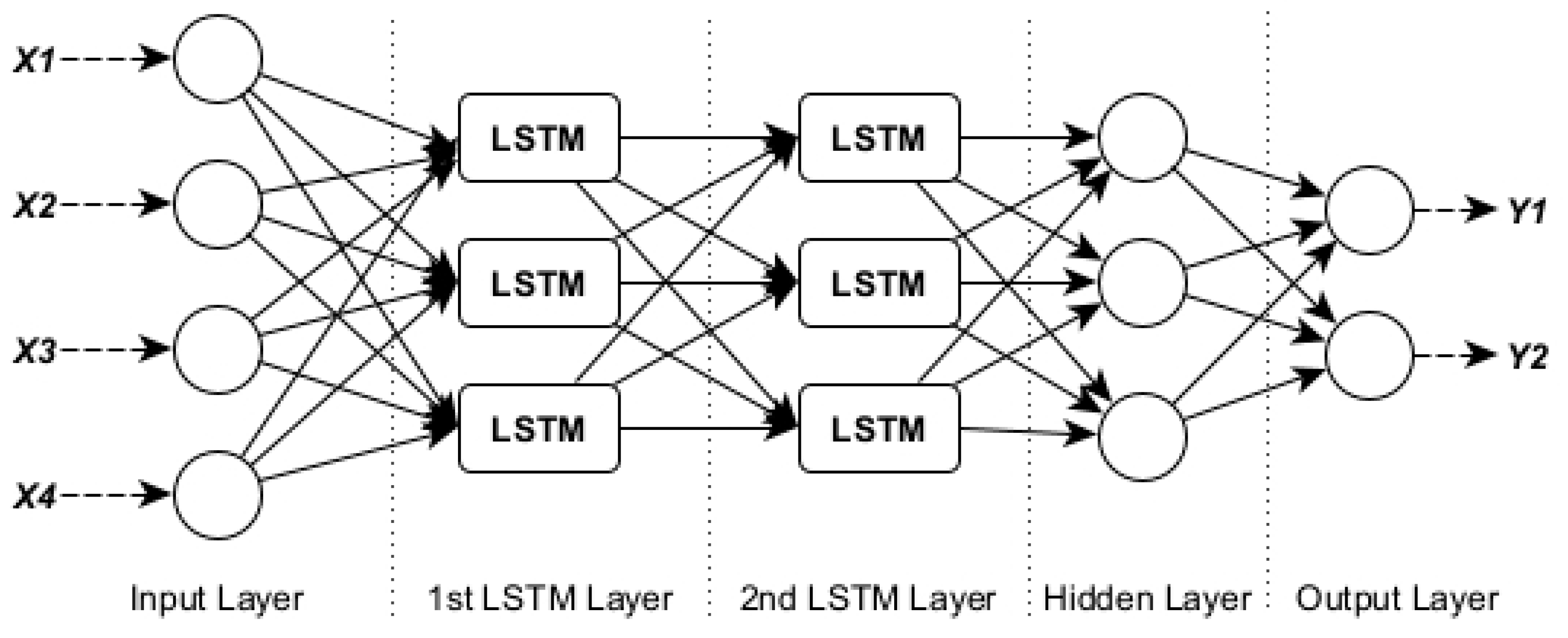
An LSTM-based DNN architecture can contain more than one LSTM cell within the network, which is called multilayer LSTM [39]. Multilayer LSTM is an extension of this model consisting of multiple hidden LSTM layers with numerous memory cells per layer. The multilayer LSTM hidden layers deepen the model, more accurately qualifying it as a deep learning strategy. The multilayer LSTM architecture illustrated in Figure 6 consists of an LSTM model with double LSTM layers [40,41]. The LSTM layer on the top outputs a sequence rather than a single value to the LSTM layer below. One output per input time step corresponds to one output time step for each input time step. Therefore, stacked LSTM was used for this study.

Another type of LSTM network is so-called bi-directional LSTM. In a regular LSTM network, the forecasting effect is lost when the network is applied to time series due to the omission of future context information and the inability to learn all sequences. Bi-directional LSTM allows each training sequence to be performed in two directions, forward and backward, being composed of two LSTM cells [42]. This structure is capable of calculating the past and future states of each input sequence cell. A bi-directional LSTM network’s hidden layer should store two values and participate in both the forward and the reverse calculations [43]. Figure 7 illustrates the architecture of bi-directional LSTM.

2.3. Evaluation Metrics

Before a forecasting model can be used in real-world applications, it must be examined and analyzed based on its type. Two important factors to keep in mind are the ability of the forecasts to accurately represent future scenarios through the precise modeling of processes, and the value of the forecasts obtained in terms of their use in decision making. Numerous point forecasts are evaluated by calculating the forecast error using various error measures. The most common error metrics are the RMSE and MAE, both of which are addressed in the next section. Other available error measurements include the mean square error, mean bias error, and mean absolute percentage error.

The RMSE is the square root of the mean of all error squares. The RMSE is widely employed and is regarded as an excellent error metric for general numerical forecasting [44]. The formula to compute the RMSE is shown in Equation (5).

$$\mathrm{R}\mathrm{M}\mathrm{S}\mathrm{E}=\sqrt{\frac{1}{n}{\sum }_{i=1}^n{(S_i-O_i)}^2}$$

(5)

In Formula (1), O_i is the observations, S_i is the projected values of a variable, and n is the number of accessible observations for analysis. As the RMSE is scale-dependent, it can only be used to compare the forecasting errors of different models or model configurations for a single variable and not between variables.

The MAE is a popular metric due to the fact that, similar to the RMSE, the error value units correspond to the anticipated goal value units. MAE changes are linear and, hence, intuitive, unlike RMSE changes. The MSE and RMSE penalize higher errors to a greater extent, with the square of the error value inflating or increasing the mean error value. For the MAE, different error sizes are not weighted differently; rather, the scores increase linearly as the number of errors increases [44]. The general formulation of the MAE value is shown in Equation (6).

$$\mathrm{M}\mathrm{A}\mathrm{E}=\frac{1}{n}\sum _{i=1}^n{\left|y_1-\widehat{y_1}\right|}^2$$

(6)

In addition to the RMSE and MAE, we also used R² (the coefficient of determination) and Willmott’s index of agreement (WIA). R² and WIA are two commonly used measures of model efficacy when evaluating time-series models. R² provides an estimate of the proportion of the dependent variable’s variability that is explained by the model’s independent variable(s) [45]. In time-series modeling, however, data autocorrelation can result in high R² values, even if the model does not adequately suit the data. WIA can therefore provide a complementary measure of model performance by assessing the agreement between observed and predicted values while accounting for the overall data variability [46]. A high WIA score indicates a decent fit between observed and predicted values, showing that the model captured the data patterns accurately. It is essential to interpret R² and WIA within the specific context of the problem being analyzed and consider other measures of model performance.

2.4. SHapley Additive exPlanations (SHAP)

SHAP values (Shapley additive explanations) are a cooperative game-theory-based strategy used to improve the interpretability and transparency of machine learning models. The essence of Shapley values is to measure the contributions to the final outcome made by each coalition member separately while ensuring that the sum of those contributions equals the final outcome [47]. Compared to the common approaches for measuring attribute contribution, such as sensitivity analysis, Shapley values provide a more comprehensive and interpretable way to measure the contribution of each input feature to the output of a model, including LSTM models. While sensitivity analysis can help identify the most influential features on a model’s output, it does not provide a clear quantitative measure of their contribution, and it may not be able to capture interactions between features. Shapley values, on the other hand, provide a method to decompose the model output into the contributions of each input feature, accounting for interactions between features. This can be particularly useful for understanding the behavior of complex models such as LSTM models. Shapley values can also be used to identify which features have a positive or negative impact on the model’s output and the magnitude of their contribution.

Linear models, for instance, might utilize their coefficients as a measure for the overall significance of each characteristic, but they are scaled with the scale of the variable, which can lead to distortions and misinterpretations. Additionally, the coefficient cannot account for the local significance of the feature and how it varies when its value decreases or increases [47]. The same holds true for the feature importance of tree-based models, which is why SHAP values are beneficial for model interpretability. Other techniques utilized to describe models include permutation significance and partial dependence plots. Below are listed several advantages of employing SHAP values as opposed to other methods [48]:

• Global interpretability: SHAP scores not only indicate the significance of a trait but also if it has a positive or negative effect on predictions.
• Local interpretability: One can calculate SHAP values for each individual prediction and understand how each feature contributes to that prediction. Other strategies merely display findings aggregated throughout the entire dataset.
• SHAP values can be used to explain a wide range of models, such as linear models (e.g., linear regression); tree-based models (e.g., XGBoost); and neural networks, but other techniques can only be used to explain a restricted number of model types.

The SHAP method demonstrate how to obtain the projected base value $E\left[f\left(z\right)\right]$ if no features of the current output $f\left(x\right)$ are known. Figure 8 illustrates the SHAP value distribution.

The diagram in Figure 8 depicts a single arrangement of the SHAP method. When the model is nonlinear or the input features are not independent, the order in which the features are added to the prediction model is significant, and the SHAP values are derived by averaging the values across all possible orderings [49]. The SHAP values themselves are derived by averaging the I values across all possible orderings using Formula (7).

$$f_z\left(z^{\prime }\right)=f\left(h_x\left(s^{\prime }\right)\right)=E\left[F\left(Z\right)|Z_s\right],$$

(7)

The SHAP value calculation method presented in Formula (7) implies a simpler input mapping, $h_x\left(z^{\prime }\right)=z_S$, where $z_S$ contains missing values for non-significant features. The SHAP formula approximates $f\left(z_S\right)$ with $E\left[F\left(Z\right)|Z_s\right]$, because the majority of models cannot accommodate arbitrary patterns of missing input values.

The concept SHAP values is intended to correspond closely to Shapley regression, Shapley sampling, and quantitative input influence feature attributions, while also permitting linkages with LIME, DeepLIFT, and layer-wise relevance propagation [50]. Hence, the precise calculation of SHAP values is difficult. However, SHAP values can be approximated by incorporating the learning results from current additive feature attribution methods. Therefore, feature independence and model linearity are two optional assumptions that facilitate the computation of anticipated values by the following formula:

$$\begin{gathered} f\left(h_x\left(z^{\prime }\right)\right)=E\left[F\left(Z\right)|Z_s\right] \\ =E_{z_{\stackrel{-}{S}}|z_S}[f(z)] \\ \approx E_{z_{\stackrel{-}{S}}}[f(z)] \\ \approx {f([}_{z_{\stackrel{-}{S}}},E[z_{\stackrel{-}{S}}]]) \end{gathered}$$

(8)

3. Results and Discussion

3.1. Experimental Settings

The first step of the experiment was to prepare the data for time-series analysis and arrange a set of scenarios to explore various combinations of parameters and algorithms in order to obtain optimal results in terms of training time and model performance. To perform time-series analysis using LSTM, the data needed to be represented in suitable formats. The suitable format required the dataset to be framed as a supervised learning task with normalized input variables. In this phase, the dataset was framed as a supervised learning problem by predicting the energy usage for the next few hours given the energy usage of the current and/or previous few hours and corresponding parameters.

In this experiment, to explore the results of various settings on the input data, we further transformed the input data using various sub-sequential formats. The sliding windows technique was used to achieve these sub-sequential formats.

Table 2. The data input scenarios.

Scenario	Number of Windows	Explanation
1	1	Using the current hour of energy usage
2	4	Using the last 4 h of energy usage
3	8	Using the last 8 h of energy usage
4	12	Using the last 12 h of energy usage
5	16	Using the last 16 h of energy usage

shows the various input data formats used in this study. The number of windows represents the number of inputs assigned to the LSTM model. The input data were represented as a vector, as illustrated in Figure 4.

The various sets of input data outlined in Table 2 were then evaluated using three different LSTM architectures, i.e., single-layer LSTM, double-layer LSTM, and bi-directional LSTM. To obtain the optimal hyperparameter settings, GridSearch, which is available from the Python Scikit-Learn package, was implemented. We implemented GridSearch on single-layer LSTM and then applied the best hyperparameter combination to the other two LSTM architectures. The hyperparameters evaluated using the GridSearch function were the number of LSTM units and the dropout value. We used the hourly energy usage dataset covering a single year, which contained 4.380 records. We considered 10 months of data from January to October, or approximately 3600 records (82% of the dataset), as the training dataset, and the rest were used for the testing dataset.

Table 3. Performance summary of parameter combinations for LSTM using GridSearch.

Rank	Number of LSTM Units	Dropout Value	RMSE	Std. Dev
1	64	0.1	0.0074	0.0006
2	128	0.1	0.0076	0.0005
3	128	0.2	0.0076	0.0007
4	32	0.2	0.0077	0.0007
5	16	0.1	0.077	0.0007
6	64	0.2	0.077	0.0008
7	32	0.1	0.078	0.0008
8	16	0.2	0.079	0.0007

summarizes the results of the GridSearch operation. Based on the findings presented in Table 3, the optimum hyperparameters with the lowest RMSE were obtained, i.e., 64 LSTM units and a 0.1 dropout value. Since each LSTM configuration was run several times, Table 3 also contains the standard deviation of the RMSE score during the experiments.

3.2. LSTM Model Evaluation Results

The three LSTM architectures evaluated in this study were implemented using the Python programming language and the TensorFlow framework. Based on the best results of the GridSearch operation, the learning model of each LSTM architecture had 64 units of LSTM cells. To overcome the overfitting problem, the models were run using a dropout value of 0.1. Finally, the models contained one dense (fully connected) layer to link the neurons within the dropout layer with the output layer. After 50 iterations (epochs) of training, the performance of the three LSTM architectures in terms of the mean squared error values can be seen in Figure 9. Based on the results, the architecture with a double LSTM layer achieved the lowest RMSE score. However, the performance differences between the three architectures were very small.

Figure 9 depicts the performance of the single-layer LSTM, double-layer LSTM, and bi-directional LSTM in terms of the average RMSE score for each feature window scenario outlined in Table 2.

Table 4. Results comparison of three LSTM architectures with various input settings.

LSTM Architecture	Number of Windows	RMSE	Std. Dev.
Singe-layer	1	0.13	0.0005
	4	0.10	0.0006
	8	0.09	0.0005
	12	0.08	0.0007
	16	0.08	0.0006
Double-layer	1	0.11	0.0007
	4	0.09	0.0006
	8	0.08	0.0006
	12	0.08	0.0007
	16	0.07	0.0008
Bi-directional	1	0.14	0.0008
	4	0.12	0.0007
	8	0.10	0.0006
	12	0.08	0.0007
	16	0.07	0.0006

provides more detailed insight into the performance of each architecture with various data input settings. From the information outlined in Table 4, it can be seen that for each LSTM architecture, increasing the number of feature windows resulted in smaller validation errors (RMSE scores), with a small standard deviation of errors. However, a larger feature window also increased the dimensions of the training data, which increased the training time.

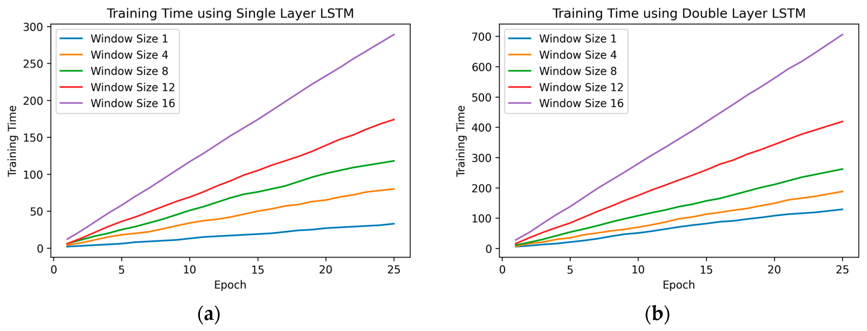
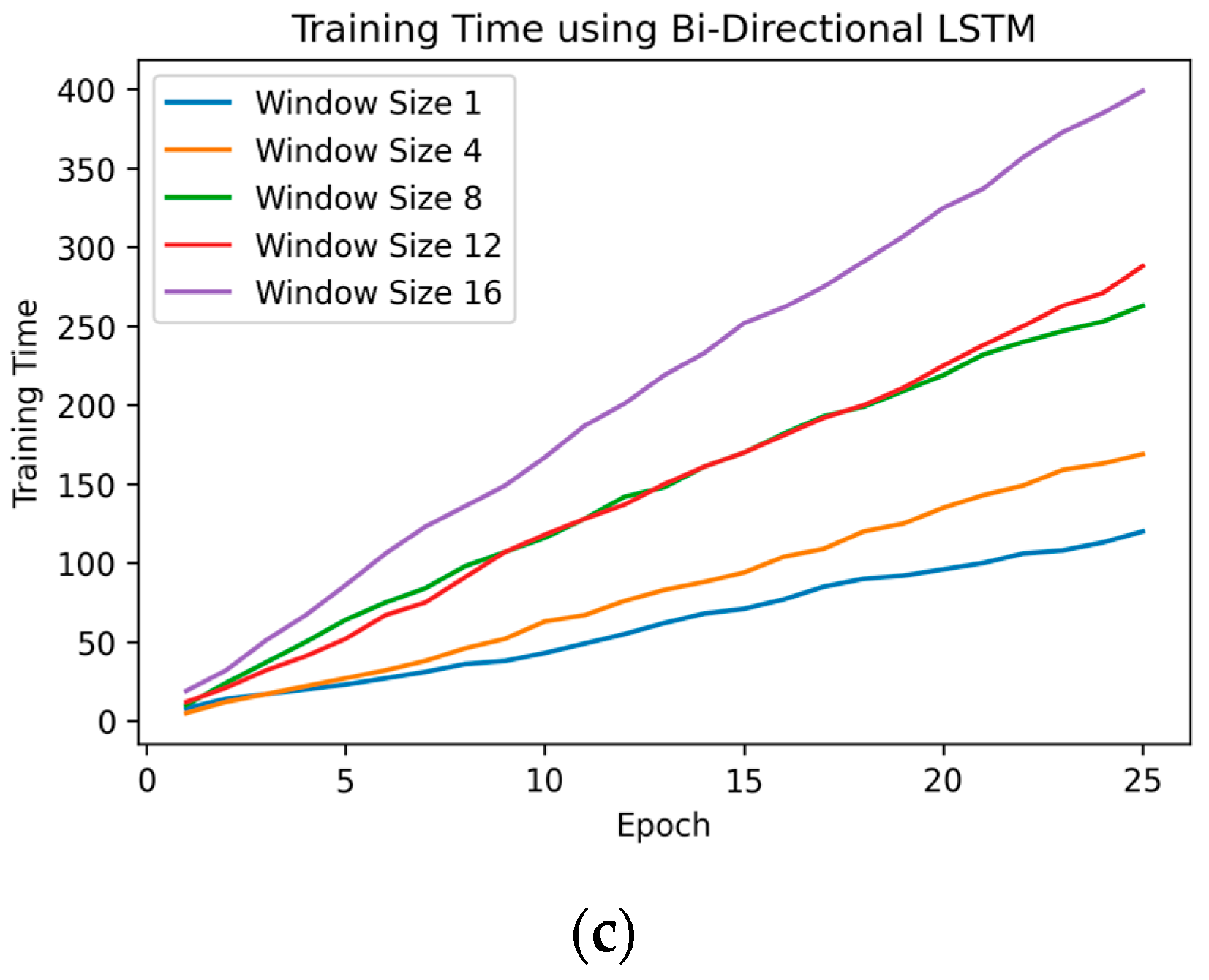
From Table 4, we can see that the number of windows was in line with the RMSE metrics, which meant that larger windows yielded better model performance. Nevertheless, adding more windows increased the training time of the model. For more detailed insight, we provide information on the training time of each architecture for each feature window size in Figure 10. From Figure 10, it can be seen that the pattern of the training time for each architecture was linear, and the values were similar.

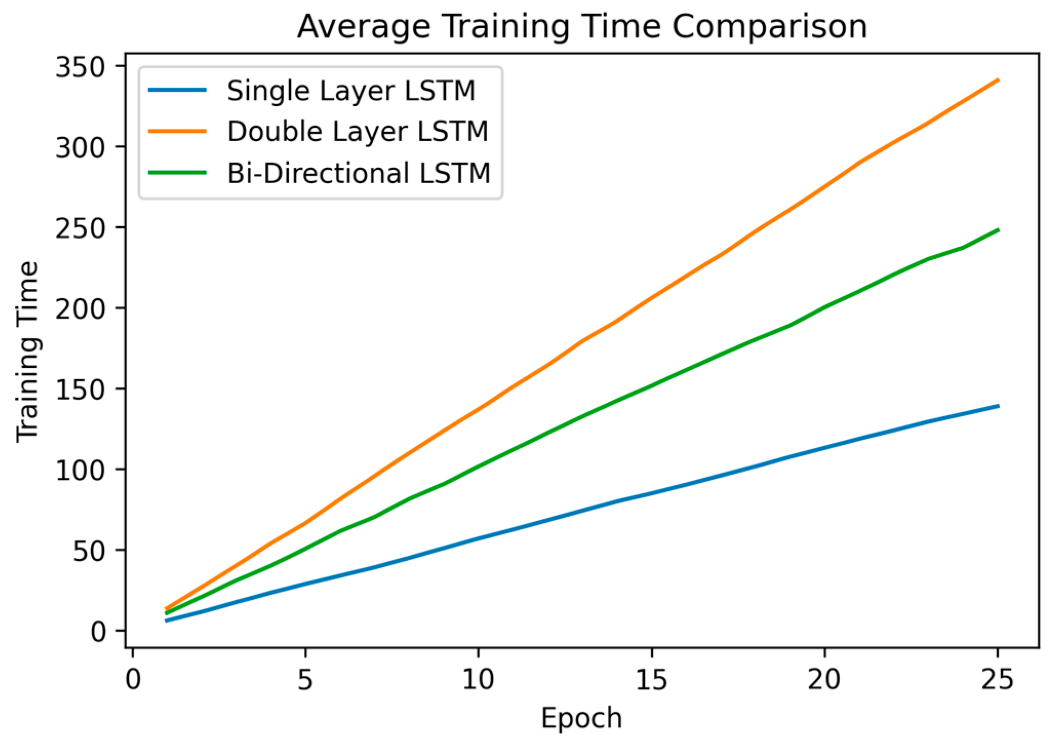
For further analysis, we investigated the average training time of each architecture under various input scenarios, as outlined in Table 4. Figure 10 shows the performance evaluation in terms of the average training time of each LSTM architecture with different input data settings. From these graphs, it can be seen that the training time for each architecture was in line with the number of feature windows. Furthermore, there was no significant difference in the training time for the single- and double-layer LSTM architectures. With only a slight difference in model performance, as illustrated in Figure 11, double-layer LSTM required a training time that was approximately three times longer than that of single-layer LSTM. Therefore, we could conclude that adding more LSTM layers would significantly affect the training time but provide only small improvements in the model performance.

For additional evaluation, we compared our LSTM models to other machine learning models proposed in previous research using the same dataset. Detailed results of the comparison with a previous study are presented in

Table 5. Comparisons with a previous study.

Reference	Model	Training				Testing
		RMSE	MAE	R2	WIA	RMSE	MAE	R2	WIA
Satishkumar et al. [51]	SVM	0.89	0.51	-	-	0.97	0.54	-	-
	RF	0.51	0.15	-	-	0.62	0.36	-	-
	Cubist	0.11	0.03	-	-	0.24	0.05	-	-
Our study	Single-layer LSTM	0.08	0.05	0.97	0.95	0.08	0.04	0.97	0.94
	Double-layer LSTM	0.07	0.04	0.98	0.96	0.08	0.04	0.97	0.95
	Bi-directional LSTM	0.07	0.05	0.98	0.96	0.08	0.03	0.98	0.95

. Satishkumat et al. [51] proposed several machine learning models, including support vector machine (SVM), K-nearest neighbors (KNNs), random forest, and the Cubist regression model. In their experiments, they obtained the best model performance using the Cubist regression model, with RMSE and MAE validation scores of 0.11 and 0.03, respectively, for training data. The validation using testing data showed that the Cubist regression model also yielded the best performance, with RMSE and MAE scores of 0.24 and 0.05, respectively.

Comparing our models to those in this previous study, we discovered that our models achieved a higher performance in terms of the RMSE score by 0.08, 0.07, and 0.07 for single-layer LSTM, double-layer LSTM, and bi-directional LSTM, respectively. It should be noted that due to the differences in the methods/algorithms used and their respective parameters, this comparison may have provided inaccurate information. However, this comparison, as shown in Table 5, suggested that constructing a model of energy usage from the perspective of time series using the LSTM approach had promising results, which were close to those of another regular supervision-based machine learning model. In addition, the R² and WIA scores of the LSTM model were measured to provide a more comprehensive performance evaluation. The high R² and WIA scores presented in Table 5 show that the proposed LSTM models could effectively forecast future values. This indicated that the models accurately forecast time-series data patterns.

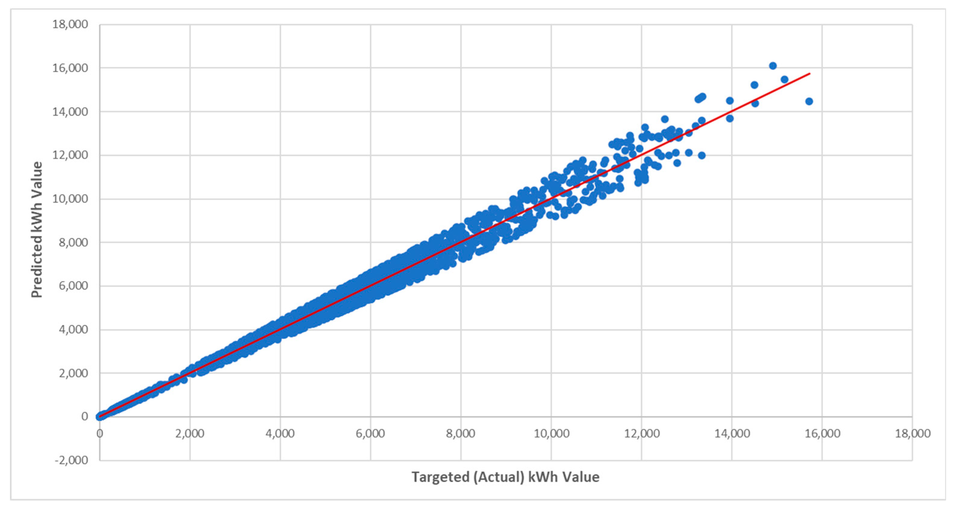
For the further evaluation of our models, Figure 12 shows a comparison of the targeted values and predicted values of energy usage in kWh. The graphic in Figure 12 was generated based on the past two months of energy usage data from the testing dataset. Figure 12 shows that there were only small differences between the predicted and target kWh values over the entire timeline. Due to the space limitations of the graph, the line in Figure 12 represents the average value of the electricity load on a daily basis. Hence, in addition to Figure 12, Figure 13 shows a scatterplot representing a comparison of the target and predicted values for all the datapoints in the testing dataset.

3.3. XAI Parameters Analysis

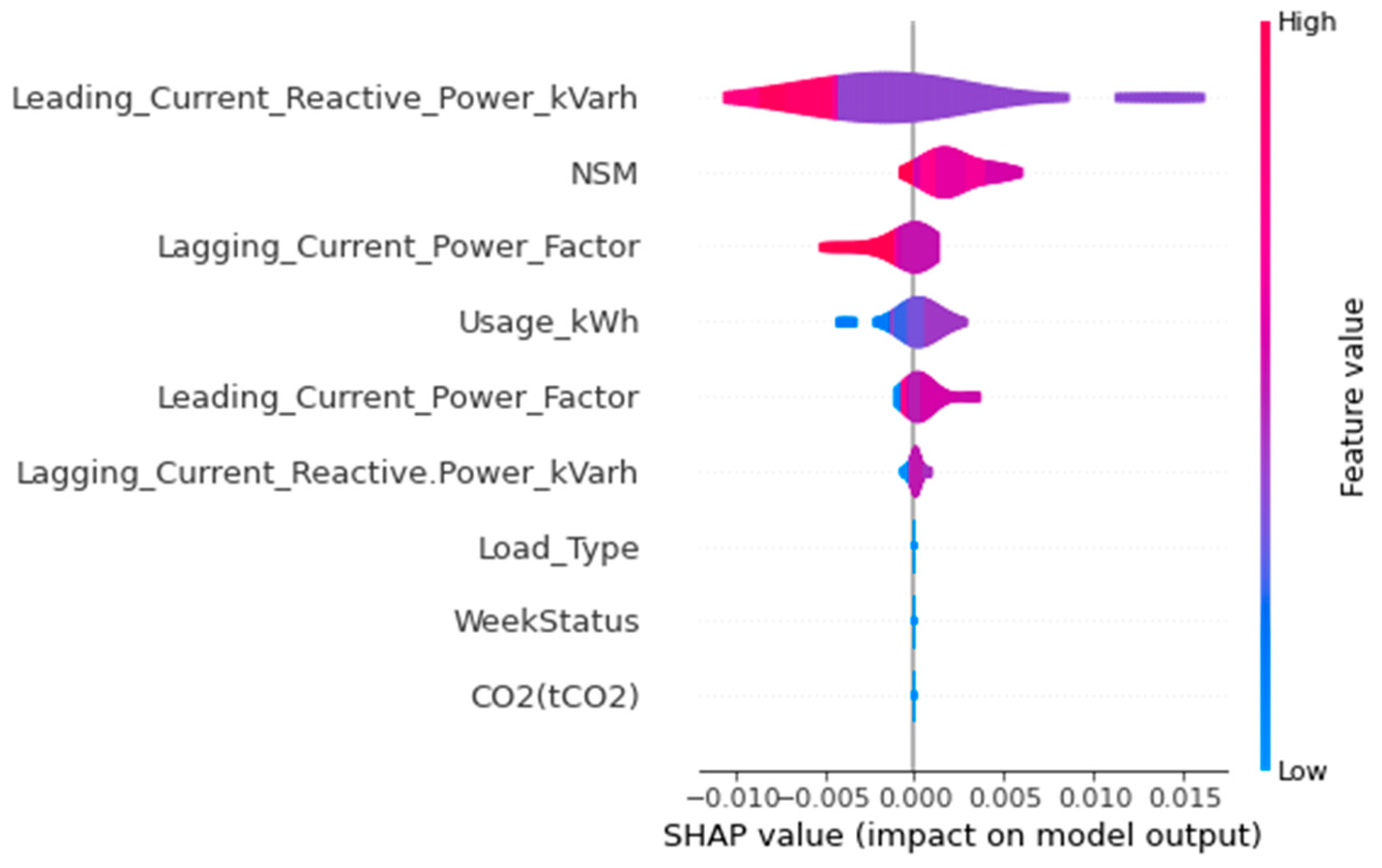
To investigate the model’s explainability, the SHAP method was implemented to improve the interpretability of the machine learning models so that the effect of each predictor variable on the model output could be investigated. The SHAP values represented each variable’s contribution to the forecasting model. Figure 14 depicts summary plots that include all of the characteristics that were used together with the corresponding SHAP values for each model. The SHAP value summary plot illustrates the distribution of every SHAP value that was computed for every characteristic in every sample. In the SHAP graphs depicted in Figure 14, each input feature is represented by a vertical bar, whose position on the x-axis indicates the SHAP value, corresponding to its contribution to the model’s output [45]. Positive and negative SHAP values indicate that the feature increased or decreased the model output, respectively. The magnitude of the SHAP value indicates the strength of the effect. The color of each bar represents the feature’s value relative to the other instances in the dataset, with blue indicating low values or negative effects, and red indicating high values or positive effects [52]. Therefore, the color scheme provides an additional visual cue to help interpret the contributions of each feature and understand the relationship between their values and the model’s predictions. Overall, the SHAP plot provided a comprehensive and easily interpretable way to understand the factors that drove the model’s predictions, which could improve the transparency, interpretability, and trustworthiness of the machine learning models.

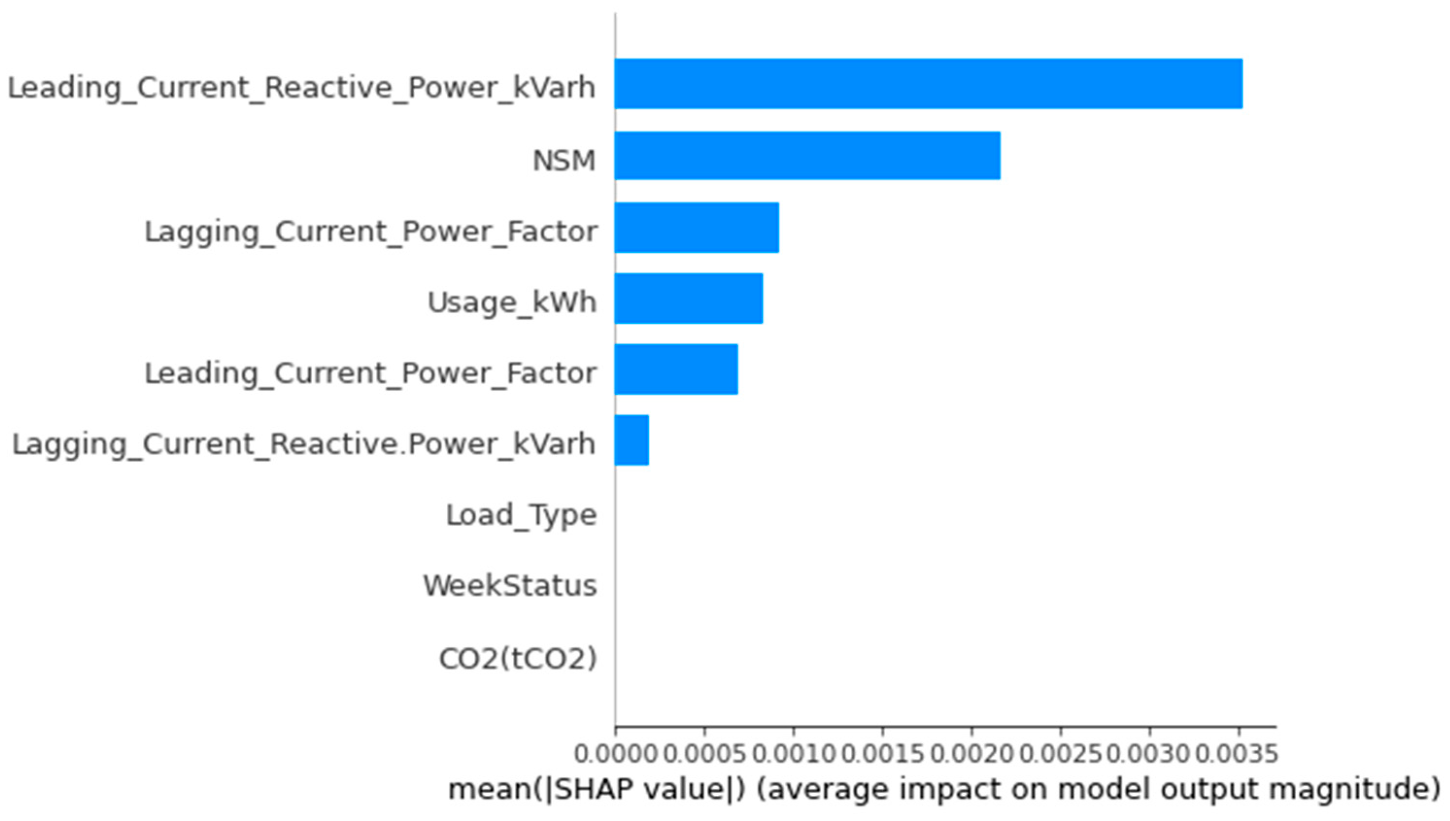
Figure 14 provides a visual representation of the distribution of SHAP values for each feature, while also ranking the features according to the mean absolute SHAP values in descending order. While the vertical lines show the feature importance, the horizontal position indicates the effect of each feature on the forecasting value. Hence, for instance, a lower value of leading current reactive power had a positive impact on predicting a high value of energy demand. As an alternative to the summary plot shown above in Figure 14, a simpler plot of feature importance is presented in Figure 15. In Figure 14, the variables that were deemed to be the most important are shown in decreasing order on a variable significance plot. The variables at the top had a greater impact on the model than those at the bottom.

According to the SHAP value visualization in Figure 15, two attributes, namely the leading current reactive power and the number of seconds from midnight (NSM), had strong significance for the model output. Four attributes had medium importance, i.e., lagging current power, energy usage, leading current power, and lagging current reactive power. In contrast to the high-importance features, the SHAP values in Figure 15 also revealed the least important features, which had almost no effect on the forecasting model. From the graphic in Figure 15, it can be seen that three features had no effect on the forecasting model, namely load type, CO₂, and weekly status.

4. Conclusions

For the purposes of energy management and optimization in industry, developing an accurate forecasting model of energy use is one of the most crucial challenges. Therefore, we developed highly accurate forecasting models for the hourly usage of energy in the steel sector. The energy usage forecasting models were based on LSTM techniques, including single-layer LSTM, double-layer LSTM, and bi-directional LSTM. The experimental results showed that the best LSTM architecture was double-layer LSTM, with hyperparameter configurations of 64 LSTM units and a 0.1 dropout value. Furthermore, a comparison with a previous study confirmed that our models achieved the lowest RMSE scores by up to 0.08, 0.07, and 0.07 for single-layer LSTM, double-layer LSTM, and bi-directional LSTM, respectively. According to the prediction results, employing LSTM for time-series or sequential data provided more accurate results. However, the complex architecture of LSTM required more extensive computation resources and training time for the prediction model to converge.

In addition, interpretability analysis using XAI has the potential to play a significant role in supporting the managerial aspect of energy usage forecasting. Therefore, we conducted an XAI analysis to provide a more transparent and easily interpretable explanation of the underlying mechanisms and decision-making processes, which could be valuable for stakeholders in the energy sector. The XAI analysis revealed that two parameters, namely leading current reactive power and the number of seconds from midnight, had strong significance for the model output. Finally, it is expected that our study could be useful for industry practitioners, providing LSTM models for accurate energy forecasting and offering insight for policymakers and industry leaders so that they can make more informed decisions about resource allocation and investment, develop more effective strategies for reducing energy consumption, and support the transition toward sustainable development.

However, it is important to consider the trade-offs between interpretability and predictive performance when selecting and designing XAI models. Further research is needed to develop and evaluate explainable models that are accurate and transparent and to understand the potential benefits and challenges of using these models in the energy sector.

References

1. Chen, C.; Pinar, M.; Stengos, T. Renewable Energy Consumption and Economic Growth Nexus: Evidence from a Threshold Model. Energy Policy 2020, 139, 111295. [Google Scholar] [CrossRef]
2. Chen, C.; Zuo, Y.; Ye, W.; Li, X.; Deng, Z.; Ong, S.P. A Critical Review of Machine Learning of Energy Materials. Adv. Energy Mater. 2020, 10, 1903242. [Google Scholar] [CrossRef]
3. Ahmad, T.; Zhang, D.; Huang, C.; Zhang, H.; Dai, N.; Song, Y.; Chen, H. Artificial Intelligence in Sustainable Energy Industry: Status Quo, Challenges and Opportunities. J. Clean. Prod. 2021, 289, 125834. [Google Scholar] [CrossRef]
4. Kandananond, K. Electricity Demand Forecasting in Buildings Based on Arima and ARX Models. In Proceedings of the 8th International Conference on Informatics, Environment, Energy and Applications—IEEA’19, Osaka, Japan, 16–19 March 2019. [Google Scholar] [CrossRef]
5. Lü, X.; Lu, T.; Kibert, C.J.; Viljanen, M. Modeling and Forecasting Energy Consumption for Heterogeneous Buildings Using a Physical–Statistical Approach. Appl. Energy 2015, 144, 261–275. [Google Scholar] [CrossRef]
6. Debnath, K.B.; Monjur, M. Forecasting Methods in Energy Planning Models. Renew. Sustain. Energy Rev. 2018, 88, 297–325. [Google Scholar] [CrossRef]
7. Abdel-Jaber, H.; Devassy, D.; Al Salam, A.; Hidaytallah, L.; El-Amir, M. A Review of Deep Learning Algorithms and Their Applications in Healthcare. Algorithms 2022, 15, 71. [Google Scholar] [CrossRef]
8. Fisher, C.K.; Smith, A.M.; Walsh, J.R. Machine Learning for Comprehensive Forecasting of Alzheimer’s Disease Progression. Sci. Rep. 2019, 9, 13622. [Google Scholar] [CrossRef]
9. Scher, S.; Messori, G. Predicting Weather Forecast Uncertainty with Machine Learning. Q. J. R. Meteorol. Soc. 2018, 144, 2830–2841. [Google Scholar] [CrossRef]
10. Ghoddusi, H.; Creamer, G.G.; Rafizadeh, N. Machine Learning in Energy Economics and Finance: A Review. Energy Econ. 2019, 81, 709–727. [Google Scholar] [CrossRef]
11. Yang, X.; Wang, Z.; Zhang, H.; Ma, N.; Yang, N.; Liu, H.; Zhang, H.; Yang, L. A Review: Machine Learning for Combinatorial Optimization Problems in Energy Areas. Algorithms 2022, 15, 205. [Google Scholar] [CrossRef]
12. Luo, B.; Wang, H.; Liu, H.; Li, B.; Peng, F. Early Fault Detection of Machine Tools Based on Deep Learning and Dynamic Identification. IEEE Trans. Ind. Electron. 2019, 66, 509–518. [Google Scholar] [CrossRef]
13. Schwendemann, S.; Amjad, Z.; Sikora, A. A Survey of Machine-Learning Techniques for Condition Monitoring and Predictive Maintenance of Bearings in Grinding Machines. Comput. Ind. 2021, 125, 103380. [Google Scholar] [CrossRef]
14. Loukatos, D.; Kondoyanni, M.; Alexopoulos, G.; Maraveas, C.; Arvanitis, K.G. On-Device Intelligence for Malfunction Detection of Water Pump Equipment in Agricultural Premises: Feasibility and Experimentation. Sensors 2023, 23, 839. [Google Scholar] [CrossRef]
15. He, M.; He, D. Deep Learning Based Approach for Bearing Fault Diagnosis. IEEE Trans. Ind. Appl. 2017, 53, 3057–3065. [Google Scholar] [CrossRef]
16. Bertolini, M.; Mezzogori, D.; Neroni, M.; Zammori, F. Machine Learning for Industrial Applications: A Comprehensive Literature Review. Expert Syst. Appl. 2021, 175, 114820. [Google Scholar] [CrossRef]
17. Mosavi, A.; Salimi, M.; Ardabili, S.F.; Rabczuk, T.; Shamshirband, S.; Varkonyi-Koczy, A.R. State of the Art of Machine Learning Models in Energy Systems, a Systematic Review. Energies 2019, 12, 1301. [Google Scholar] [CrossRef]
18. Fouilloy, A.; Voyant, C.; Notton, G.; Motte, F.; Paoli, C.; Nivet, M.-L.; Guillot, E.; Duchaud, J.-L. Solar Irradiation Prediction with Machine Learning: Forecasting Models Selection Method Depending on Weather Variability. Energy 2018, 165, 620–629. [Google Scholar] [CrossRef]
19. Zhang, D.; Han, X.; Deng, C. Review on the Research and Practice of Deep Learning and Reinforcement Learning in Smart Grids. CSEE J. Power Energy Syst. 2018, 4, 362–370. [Google Scholar] [CrossRef]
20. Wang, H.; Lei, Z.; Zhang, X.; Zhou, B.; Peng, J. A Review of Deep Learning for Renewable Energy Forecasting. Energy Convers. Manag. 2019, 198, 111799. [Google Scholar] [CrossRef]
21. Véstias, M.P.; Duarte, R.P.; de Sousa, J.T.; Neto, H.C. Moving Deep Learning to the Edge. Algorithms 2020, 13, 125. [Google Scholar] [CrossRef]
22. Wang, F.; Zhang, Z.; Liu, C.; Yu, Y.; Pang, S.; Duić, N.; Shafie-Khah, M.; Catalão, J.P. Generative Adversarial Networks and Convolutional Neural Networks Based Weather Classification Model for Day Ahead Short-Term Photovoltaic Power Forecasting. Energy Convers. Manag. 2019, 181, 443–462. [Google Scholar] [CrossRef]
23. Zhang, R.; Li, G.; Ma, Z. A Deep Learning Based Hybrid Framework for Day-Ahead Electricity Price Forecasting. IEEE Access 2020, 8, 143423–143436. [Google Scholar] [CrossRef]
24. Abiodun, O.I.; Jantan, A.; Omolara, A.E.; Dada, K.V.; Mohamed, N.A.; Arshad, H. State-of-the-Art in Artificial Neural Network Applications: A Survey. Heliyon 2018, 4, e00938. [Google Scholar] [CrossRef]
25. Martens, J.; Sutskever, I. Training Deep and Recurrent Networks with Hessian-Free Optimization; Lecture Notes in Computer Science; Springer: Berlin/Heidelberg, Germany, 2012; pp. 479–535. [Google Scholar] [CrossRef]
26. Xu, J.; Jiang, Y.; Yang, C. Landslide Displacement Prediction during the Sliding Process Using XGBoost, SVR and RNNs. Appl. Sci. 2022, 12, 6056. [Google Scholar] [CrossRef]
27. Hochreiter, S.; Schmidhuber, J. Long Short-Term Memory. Neural Comput. 1997, 9, 1735–1780. [Google Scholar] [CrossRef]
28. Sherstinsky, A. Fundamentals of Recurrent Neural Network (RNN) and Long Short-Term Memory (LSTM) Network. Phys. D Nonlinear Phenom. 2020, 404, 132306. [Google Scholar] [CrossRef]
29. Kim, T.-Y.; Cho, S.-B. Predicting Residential Energy Consumption Using CNN-LSTM Neural Networks. Energy 2019, 182, 72–81. [Google Scholar] [CrossRef]
30. Le, T.; Vo, M.T.; Vo, B.; Hwang, E.; Rho, S.; Baik, S.W. Improving Electric Energy Consumption Prediction Using CNN and Bi-LSTM. Appl. Sci. 2019, 9, 4237. [Google Scholar] [CrossRef]
31. Angelov, P.; Soares, E. Towards Explainable Deep Neural Networks (XDNN). Neural Netw. 2020, 130, 185–194. [Google Scholar] [CrossRef] [PubMed]
32. Pavone, A.; Plebe, A. How Neurons in Deep Models Relate with Neurons in the Brain. Algorithms 2021, 14, 272. [Google Scholar] [CrossRef]
33. Minh, D.; Wang, H.X.; Li, Y.F.; Nguyen, T.N. Explainable Artificial Intelligence: A Comprehensive Review. Artif. Intell. Rev. 2021, 55, 3503–3568. [Google Scholar] [CrossRef]
34. Angelov, P.P.; Soares, E.A.; Jiang, R.; Arnold, N.I.; Atkinson, P.M. Explainable Artificial Intelligence: An Analytical Review. WIREs Data Min. Knowl. Discov. 2021, 11, e1424. [Google Scholar] [CrossRef]
35. Speith, T. A Review of Taxonomies of Explainable Artificial Intelligence (XAI) Methods. In Proceedings of the 2022 ACM Conference on Fairness, Accountability, and Transparency, Seoul, Republic of Korea, 21–24 June 2022. [Google Scholar] [CrossRef]
36. Ahmed, I.; Jeon, G.; Piccialli, F. From Artificial Intelligence to Explainable Artificial Intelligence in Industry 4.0: A Survey on What, How, and Where. IEEE Trans. Ind. Inform. 2022, 18, 5031–5042. [Google Scholar] [CrossRef]
37. Rehmer, A.; Kroll, A. On the Vanishing and Exploding Gradient Problem in Gated Recurrent Units. IFAC-PapersOnLine 2022, 53, 1243–1248. [Google Scholar] [CrossRef]
38. Gers, F.A.; Schmidhuber, J.; Cummins, F. Learning to Forget: Continual Prediction with LSTM. Neural Comput. 2000, 12, 2451–2471. [Google Scholar] [CrossRef] [PubMed]
39. Yu, Y.; Si, X.; Hu, C.; Zhang, J. A Review of Recurrent Neural Networks: LSTM Cells and Network Architectures. Neural Comput. 2019, 31, 1235–1270. [Google Scholar] [CrossRef]
40. Zhang, S.; Liu, X.; Xiao, J. On Geometric Features for Skeleton-Based Action Recognition Using Multilayer LSTM Networks. In Proceedings of the 2017 IEEE Winter Conference on Applications of Computer Vision (WACV), Santa Rosa, CA, USA, 24–31 March 2017. [Google Scholar] [CrossRef]
41. Turkoglu, M.O.; D’Aronco, S.; Wegner, J.; Schindler, K. Gating Revisited: Deep Multi-Layer RNNS That Can Be Trained. IEEE Trans. Pattern Anal. Mach. Intell. 2021, 44, 4081–4092. [Google Scholar] [CrossRef]
42. Graves, A.; Schmidhuber, J. Framewise Phoneme Classification with Bidirectional LSTM and Other Neural Network Architectures. Neural Netw. 2005, 18, 602–610. [Google Scholar] [CrossRef]
43. Yang, S.U. Research on Network Behavior Anomaly Analysis Based on Bidirectional LSTM. In Proceedings of the 2019 IEEE 3rd Information Technology, Networking, Electronic and Automation Control Conference (ITNEC), Chengdu, China, 15–17 March 2019. [Google Scholar] [CrossRef]
44. Karunasingha, D.S. Root Mean Square Error or Mean Absolute Error? Use Their Ratio as Well. Inf. Sci. 2022, 585, 609–629. [Google Scholar] [CrossRef]
45. Lundberg, S.M.; Lee, S.I. A Unified Approach to Interpreting Model Predictions. In Proceedings of the 31st International Conference on Neural Information Processing Systems (NIPS’17), Long Beach, CA, USA, 4–9 December 2017; Curran Associates Inc.: Red Hook, NY, USA, 2017; pp. 4768–4777. [Google Scholar]
46. Hyndman, R.J.; Athanasopoulos, G. Forecasting: Principles and Practice; OTexts: Melbourne, Australia, 2018; ISBN 978-0-646-99855-8. [Google Scholar]
47. Montgomery, D.C.; Jennings, C.L.; Kulahci, M. Introduction to Time Series Analysis and Forecasting; John Wiley & Sons: Hoboken, NJ, USA, 2015; ISBN 978-1-118-71283-8. [Google Scholar]
48. Marcilio, W.E.; Eler, D.M. From Explanations to Feature Selection: Assessing Shap Values as Feature Selection Mechanism. In Proceedings of the 2020 33rd SIBGRAPI Conference on Graphics, Patterns and Images (SIBGRAPI), Porto de Galinhas, Brazil, 7–10 November 2020. [Google Scholar] [CrossRef]
49. Van den Broeck, G.; Lykov, A.; Schleich, M.; Suciu, D. On the Tractability of Shap Explanations. J. Artif. Intell. Res. 2022, 74, 851–886. [Google Scholar] [CrossRef]
50. Adadi, A.; Berrada, M. Peeking inside the Black-Box: A Survey on Explainable Artificial Intelligence (XAI). IEEE Access 2018, 6, 52138–52160. [Google Scholar] [CrossRef]
51. Sathishkumar, V.E.; Shin, C.; Cho, Y. Efficient Energy Consumption Prediction Model for a Data Analytic-Enabled Industry Building in a Smart City. Build. Res. Inf. 2020, 49, 127–143. [Google Scholar] [CrossRef]
52. Strumbelj, E.; Kononenko, I. Explaining Prediction Models and Individual Predictions with Feature Contributions. Knowl. Inf. Syst. 2014, 41, 647–665. [Google Scholar] [CrossRef]
Figure 1. General framework/flow of the study.
Information 14 00265 g001
Figure 2. Energy usage plot based on the raw dataset: (a) 15 min intervals and (b) 1 h intervals.
Information 14 00265 g002
Figure 3. Transformation of (a) the original dataset using (b) 1 sliding window and (c) 3 sliding windows.
Information 14 00265 g003
Figure 4. Illustration of sliding windows from (a) original data format to (b) 3 sliding windows.
Information 14 00265 g004
Figure 5. The architecture of (a) an LSTM network and (b) an LSTM unit.
Information 14 00265 g005
Figure 6. An example of a multilayer LSTM architecture with 2 (double) LSTM layers and 3 LSTM units on each LSTM layer.
Information 14 00265 g006
Figure 7. The basic architecture of a bi-directional LSTM model.
Information 14 00265 g007
Figure 8. SHAP values attributing to each feature the change in the expected model prediction when conditioning that feature [49].
Information 14 00265 g008
Figure 9. The average of validation loss values during model training for each algorithm.
Information 14 00265 g009
Figure 10. Comparison of the training time required under various input data settings for (a) single-layer; (b) double-layer; and (c) bi-directional LSTM architecture.
Information 14 00265 g010aInformation 14 00265 g010b
Figure 11. The average of validation loss values during model training.
Information 14 00265 g011
Figure 12. Comparison of average target and predicted kWh values on a daily basis.
Information 14 00265 g012
Figure 13. Comparison of all datapoints of target and predicted kWh values.
Information 14 00265 g013
Figure 14. The SHAP values of each model attribute.
Information 14 00265 g014
Figure 15. The importance of each model attribute to the prediction results.
Information 14 00265 g015