Indoor Fire Detection Algorithm Based on Second-Order Exponential Smoothing and Information Fusion

Abstract

With the increasing complexity of building structures and interior materials, the danger of indoor fires has become more severe. It is effective to improve the accuracy and timeliness of fire-sensing devices in order to reduce the harm caused by fires. This paper focuses on the temporal characteristics of sensor information, creatively introducing second-order exponential smoothing into the information fusion algorithm. The RNN structure is used to fit the formula and adaptively trained with various types of fire data. Experimental results show that the proposed algorithm achieves an accuracy of 98% in fire recognition, significantly improving the accuracy of fire recognition. To avoid the issue of imbalanced positive and negative samples, this paper comprehensively evaluates parameters such as F1-score and Matthews correlation coefficient (MCC). The achieved scores are 0.97 and 0.95, respectively, indicating the algorithm’s good performance in detecting the presence or absence of fire. Furthermore, the proposed algorithm is tested for its alarm time. The experimental results show that the proposed algorithm can timely identify various types of fires and can give an alarm earlier than traditional fire alarms.

1. Introduction

Based on data from the U.S. Fire Administration, the number of fire-related deaths has been on an upward trend, with an average of 3500 people losing their lives to fires each year. A survey by the European Fire Safety Alliance found that 37% of fire safety experts believe that collective housing, such as apartments, should receive greater attention. The timely and reliable identification of fires within buildings has great practical significance. People need to spend most of their time in indoor environments such as bedrooms, offices, and living rooms. Once a fire occurs, it can pose a very serious threat to life. In addition, with the increasingly complex building structures, higher floors, and more diverse types and materials of items within buildings, the danger posed by fires has also increased.

Fires can be classified into two types: flame and smoldering. Flame is a common manifestation of fires and refers to visible flames that produce bright light and heat, as well as a large amount of smoke. The combustion energy of flame comes from the combustible materials themselves, such as wood, paper, and liquid fuels. The combustion process of open flame is usually obvious and easily detected. Smoldering fires, on the other hand, refer to the situation where combustion occurs without significant increases in temperature or visible flames. This type of fire often occurs in poorly ventilated environments, where the combustible materials contain high moisture content, such as damp cotton and other materials, or in areas with high humidity. Smoldering fires are difficult to detect but can also generate toxic gases and particles, posing a high level of danger. Therefore, in fire safety, it is necessary to improve the accuracy and timeliness of fire alarms for both types of fires.

Fire detection is mainly based on sensitive devices that collect images, aerosols, smoke and other fire-related information and respond with corresponding measurements [1]. In the field of image processing, the main features detected are the visual changes associated with a fire, such as color, brightness, shape, and spectral characteristics. For private places such as residential bedrooms, sensors are commonly used to collect environmental data for detection, which is more practical and cost-effective. Traditional warning methods often use smoke alarms. However, smoke alarms may be affected by specific fire situations and external environmental interferences. This can lead to false alarms, missed alarms, and other issues. False alarms waste the resources of fire departments and reduce the comfort of residents. Therefore, it is necessary to develop an accurate fire alarm system.

One alarm method currently known is to install both photoelectric smoke sensors and ionization smoke detectors. Ionization smoke detectors are sensitive to rapidly burning fires and primarily detect smoke particles, so they are not suitable for installation in locations where smoke is regularly produced. On the other hand, photoelectric sensors trigger alarms when smoke particles obstruct light propagation, making them more suitable for detecting smoldering fires. Inspired by this fire alarm method, the current mainstream approach to fire detection is to use information fusion methods that can be widely applied to various environments. Information fusion can be achieved through methods such as weighted averages, least squares estimation, fuzzy theory, clustering analysis, neural networks, and expert systems. This paper focuses on using artificial intelligence methods to achieve fire alarm systems. Okayama [2] first proposed a fire recognition system that introduced a three-layer neural network that uses temperature, smoke, and gas sensor data to identify fires and highlighted the advantages of using neural networks in this field, which can reflect complex input–output combinations even in the absence of relevant experiential knowledge of input–output causality. Chen and Fu [3] established a fire alarm system based on a Bayesian network (BN) model, which demonstrated the feasibility and effectiveness of a BN-based fire alarm system using powerful graphical knowledge representation and effective handling of uncertain results. Their research confirmed the feasibility and effectiveness of using input from CO, CO₂, temperature, and smoke sensors to analyze different fire probabilities in alarm systems. Nakıp and Güzeliş [4] designed a multi-sensor system consisting of gas, temperature and humidity, heat, and smoke sensors using a Raspberry Pi 3-based sensor information acquisition circuit. He also developed a neural network fire prediction system based on trend extraction, which demonstrated the advantages of trend prediction over a normal multilayer perceptron (MLP) model. Wu et al. [5] proposed a neural network that also introduced trend extraction, which was improved based on the Kendall-τ trend extraction formula [6] and achieved fire detection based on temperature, smoke, and CO sensor information. The trend-based multi-sensor fire alarm algorithm takes into account changes in sensor data as the fire develops, but the trend calculation method is relatively fixed, making it difficult to adapt to different fire situations, and data preprocessing methods, such as averaging filtering, still need to be incorporated, leading to some resource waste.

To address existing issues, we propose a multi-sensor fire alarm model from the perspective of time series analysis based on a neural network. In this paper, we select three characteristic parameters, namely carbon monoxide, temperature, and smoke concentration. Unlike previous methods that require a large amount of data preprocessing to remove sensor noise, we first analyze the trend extraction methods of time series and analyze the advantages of the second-order exponential smoothing method in processing sensor data. Then, we establish a neural network algorithm model, introducing a recurrent neural network (RNN) structure to fit the second-order exponential smoothing formula for indoor fire data. To demonstrate the superiority of the proposed algorithm, we select multiple evaluation metrics and compare them with the metrics of existing algorithms. Finally, we apply our proposed model to fire data collected from another real-world residential setting and analyze the alarm time. The results show that our algorithm can effectively identify fire incidents within a reasonable time frame, demonstrating significant advantages over traditional alarm systems.

2. Model Establishment

2.1. Trend Extraction Based on Time Series Analysis

We are able to directly collect sensor data, and during the entire process of fire development, data from different sensors belong to different sets of time series. Therefore, this study mainly focuses on classification based on the changes in time series.

In order to minimize the impact of noise on identification, the most common method for handling time series is the moving average method, whose central idea is to find the information of the time series in the data, calculate the average value, and thus identify the trend of data development. This is shown in Formula (1):

$$y\left(n\right)=\frac{1}{N}{\displaystyle \sum }_{i=0}^{N}x\left(n-i\right)$$

(1)

The variable $x\left(n-i\right)$ in the formula represents the original data at $i$ time steps before the current time point, while $y\left(n\right)$ represents the smoothed data. The parameter $N$ represents the length of the moving window, which refers to the number of data points within the window. However, the moving average method has several limitations: after smoothing, the results exhibit a significant linear trend and have a certain time delay compared to the original data; the method cannot handle well the data changes at the edges of the dataset, nor can it be applied beyond the scope of the existing dataset; it requires sufficient historical data, usually dozens of data points, which can consume a large amount of storage space in hardware implementation; and regardless of the time interval between the historical data and the current time, the same weight is assigned to the historical data, and the default data acquisition time does not affect the current detection results.

The Mann–Kendall (MK) method can be used to detect trends in time series. The MK method is a non-parametric test that does not assume any specific distribution of the data. Therefore, the MK trend test is widely used in natural time series that significantly deviate from a normal or linear distribution [7] to identify sudden changes or shifts in the trend of the time series. When dealing with fire characteristic parameters, the basic idea of the MK method is to compare the differences between adjacent data points in the time series and count the number of positive and negative values of these differences. The trend direction is determined by the sign of the difference values, and the trend magnitude is determined by the number of data points with the same sign.

For the current time points $i$ and $j$, where $j$ is earlier than $i$, it has been demonstrated that the fire sensor data can be processed using an improved Kendall formula [5] to calculate the trend values of three fire characteristic parameters. The trend extraction formula is as follows:

$$y\left(n\right)={\displaystyle \sum }_{i=0}^{N-1}{\displaystyle \sum }_{j=i+1}^{N-1}sgn\left(x\left(n-i\right)-x\left(n-j\right)\right)$$

(2)

Exponential smoothing (ES) can be used as an optimized method. ES was proposed by Robert G. Brown in 1961 [8]. The changes in time series are stable or regular; therefore, time series can be inferred sequentially. In the historical data, relatively recent data have a greater impact on the continuation of subsequent data, so different weights are assigned to data that are different in time. Exponential smoothing can be divided into three types: first-order exponential smoothing, second-order exponential smoothing, and third-order exponential smoothing. Third-order exponential smoothing considers seasonal changes in data and is suitable for non-stationary sequences with periodic fluctuations, but it is not applicable to the study in this paper.

First-order exponential smoothing is a fundamental smoothing method that utilizes the previous time’s actual value and the previous time’s first-order exponential smoothing value to generate a new output sequence [9]. The calculation formula can be expressed as follows:

$$s_i=\alpha \ast x_i+\left(1-\alpha \right)s_{i-1}$$

(3)

If we expand the Formula (3), we can observe that it can be expressed as Formula (4).

$$\begin{array}{ll}{s}_i& =\alpha x_i+\left(1-\alpha \right)s_{i-1}\\ & =\alpha x_i+\left(1-\alpha \right)[\alpha x_{i-1}+\left(1-\alpha \right)s_{i-2}]\\ & =\alpha x_i+\left(1-\alpha \right)\left[\alpha x_{i-1}+\left(1-\alpha \right)[\alpha x_{i-2}+\left(1-\alpha \right)s_{i-3}\right]]\\ & =\alpha \left[x_i+\left(1-\alpha \right)x_{i-1}+{\left(1-\alpha \right)}^2{x}_{i-2}+{\left(1-\alpha \right)}^3{s}_{i-3}\right]\\ & =\dots \\ & =\alpha {\displaystyle {\displaystyle \sum }_{j=0}^i}{\left(1-\alpha \right)}^j{x}_{i-j}\end{array}$$

(4)

In Equations (3) and (4), $s_i$ represents the smoothed value at step i, and $x_i$ represents the actual data at the current time. The initial value of $s_0$ is $x_0$. The smoothing coefficient $\alpha$ is a value between 0 and 1, and there is no established method for selecting the smoothing coefficient. It is typically chosen based on experience in practical applications, which may affect the accuracy of the results [10]. The smoothing coefficient reflects recent data changes and the smoothing effect. When $\alpha$ is closer to 0, the trend of data changes is less reflected [11], and the smoothing effect is greater, resulting in a closer approximation to a horizontal straight line. When $\alpha$ is closer to 1, the trend of data changes has a greater weight, and the smoothing effect is smaller.

This study employs a data trend extraction method based on an optimized first-order exponential smoothing approach, in which the original data and trend data are combined and input into a Trend Prediction Neural Network (TPNN). The proposed trend extraction can be expressed as Equation (5).

$$t_i^k=\gamma ·\left(x_i^k-x_i^{k-1}\right)+\left(1-\gamma \right)·t_i^{k-1}$$

(5)

It can be seen from the formula that this method is based on the idea of first-order exponential smoothing, introducing the smoothing factor $\gamma$ to retain the advantage of adaptively adjusting the weight of past time information, and is optimized to not only process past data but also incorporate the data change value from the previous moment to the current moment, thereby emphasizing the characteristics of change.

The second-order exponential smoothing method is known to have superior smoothing performance [12]. To implement this method, we need to specify the smoothing coefficients $\alpha$ and $\beta$. The equations for second-order exponential smoothing are shown in Formulas (6) and (7):

$$s_i=\alpha x_i+\left(1-\alpha \right)\left(s_{i-1}+t_{i-1}\right)$$

(6)

$$t_i=\beta \left(s_i-s_{i-1}\right)+\left(1-\beta \right)t_{i-1}$$

(7)

As shown in Formulas (4) and (5), second-order exponential smoothing is an iterative process. The trend value $t_i$ is calculated as the difference between adjacent moments based on first-order exponential smoothing and is then subjected to a new round of exponential smoothing using the parameter $\beta$. The current smoothing result takes into account both the previous smoothing value and the previous trend value and is also subjected to exponential smoothing, resulting in two rounds of smoothing calculation and better noise removal. Compared to the overall average and moving average methods, second-order exponential smoothing can not only introduce the development trend value of fires but also obtain better-smoothed sensor data values, making it suitable for fire identification based on multiple sensors.

2.2. Establishment of Neural Network Models

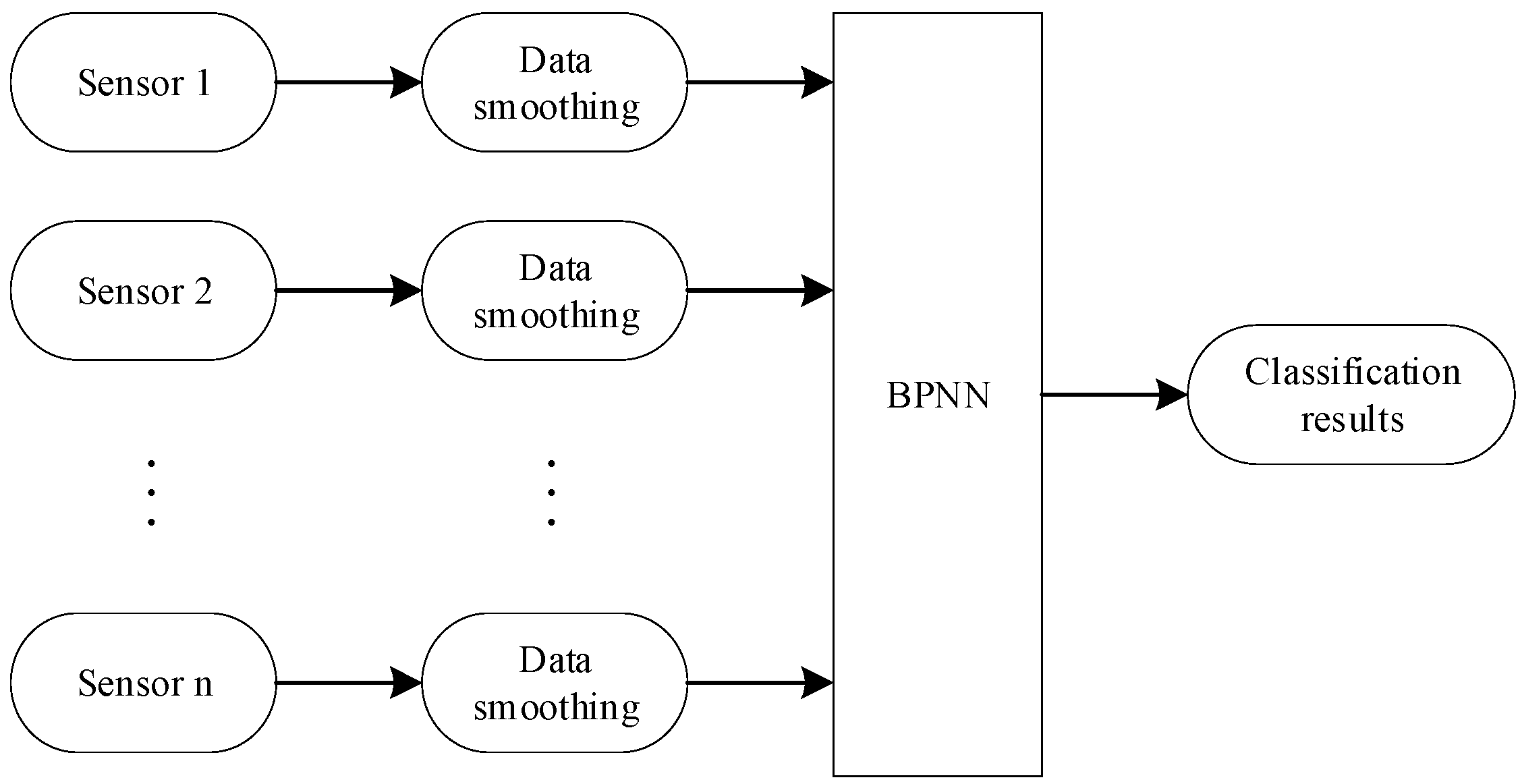
The fire classification system based on information fusion often adopts the Backpropagation (BP) neural network with strong multi-parameter fitting capability, which can effectively learn the nonlinear relationships in the data. The traditional multi-sensor fire recognition algorithm based on BP neural network has a structure shown in Figure 1, where the input data consist of selected fire feature parameters, i.e., the selected sensor data. Before being fed into the neural network, the input data need to be subjected to simple smoothing processing using methods such as moving averages or exponential smoothing, as mentioned earlier.

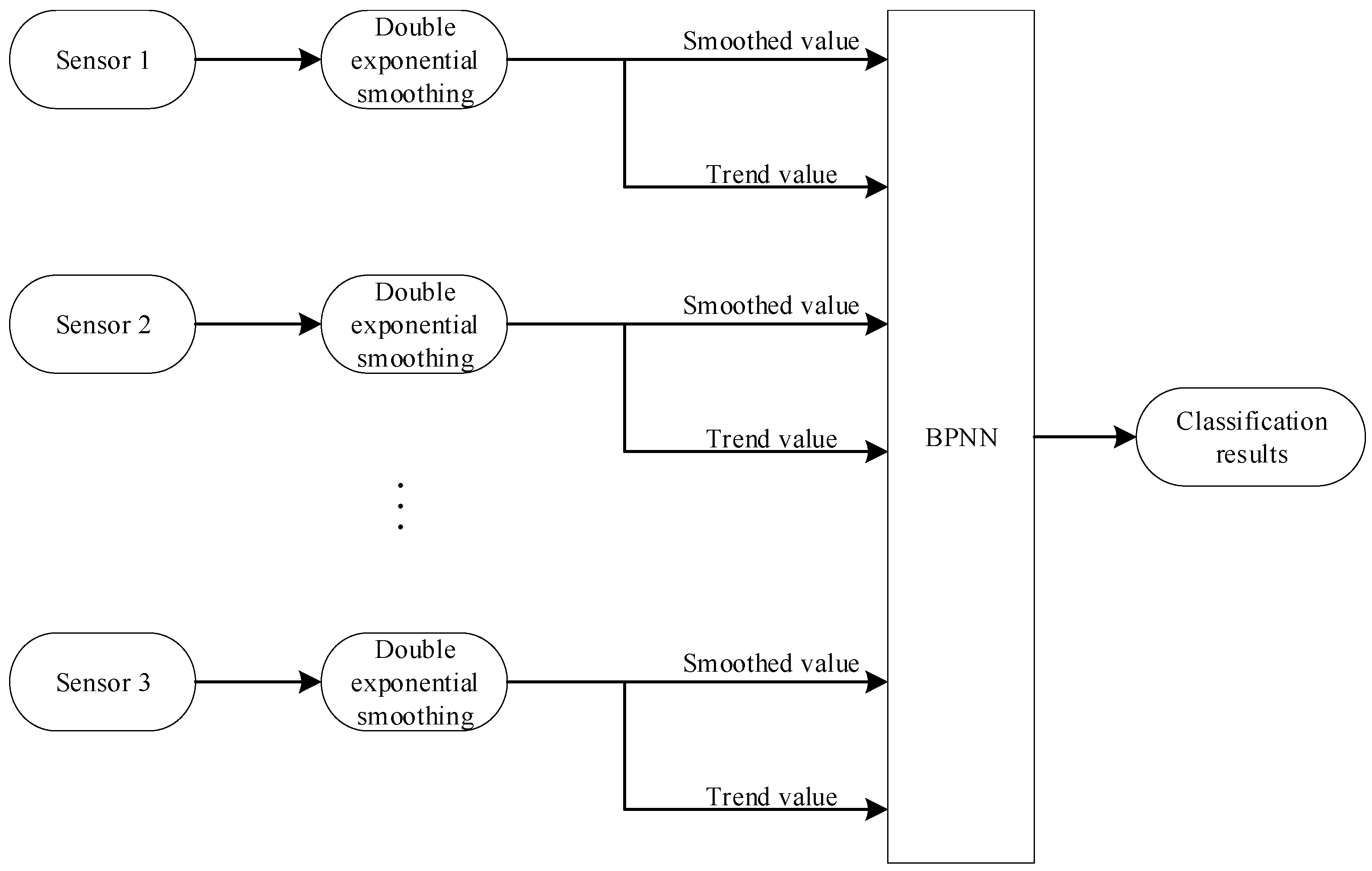
Therefore, a neural network model incorporating the second-order exponential smoothing method was established, as shown in Figure 2. The input data of the neural network are a combination of smoothed values and trend values.

In order to select the suitable smoothing parameters α and β for the proposed algorithm, the least-squares method was used for parameter fitting. The optimization algorithms commonly used for nonlinear least-squares curve fitting problems are Levenberg–Marquardt (LM), Trust Region Reflective (TRF), and Dogbox, which work by minimizing the sum of squares of the residual between predicted values and observed data.

In the field of second-order exponential smoothing for fire characteristic parameters, the values of α and β must be restricted to the range [0,1] in order for the processed fire data to have physical meaning. Furthermore, fire behavior is characterized by complexity and high nonlinearity, making the TRF and Dogbox methods suitable choices. The most appropriate method for a fire identification algorithm should be determined based on the results of fire recognition. The values of α and β fitted using TRF and Dogbox methods for the three sensors during the fire development process are shown in

Table 1. Exponential smoothing parameters fitted using TRF and Dogbox methods.

Sensor	Temperature		Smoke		CO
Parameter	α	β	α	β	α	β
TRF	0.20	0.26	0.99	0.99	0.99	0.18
Dogbox	0.06	0	0.99	1	0.99	0.18

, respectively. The α and β parameters were directly incorporated into the neural network using the quadratic exponential smoothing formula (ES-formula NN) shown in Figure 2.

In the formula of second-order exponential smoothing, α can be regarded as the memory decay factor because a larger value of α means that the model forgets historical data faster. A Recurrent Neural Network (RNN) is the most basic model structure that considers temporal relationships and has a structure similar to memory and forgetting. On the other hand, the basic BP neural network only has fully connected layers and does not have a fundamental constraint on the order of time. Therefore, introducing RNN into the fire recognition algorithm is in line with the requirement of obtaining binary classification results based on time series data.

The standard RNN model is shown in Figure 3. The forward propagation of the RNN structure is shown in Formulas (8) and (9), where $x$ represents the input data, $S$ represents the hidden layer data, $W$ and $b$ are weight and bias parameters, and $\sigma$ refers to the activation function used in the hidden layer, while ${\sigma }_o$ refers to the activation function used in the output layer.

$$S_t=\sigma \left(W_{IH}*x_t+W_{HH}*S_{t-1}+b_h\right)$$

(8)

$$y_t={\sigma }_o\left(W_{HO}{S}_t+b_o\right)$$

(9)

The input of the RNN model is a time series $\left\{\cdots ,x_{t-1},x_t,x_{t+1},\cdots \right\}$, and the hidden layer of the model stores the system state, playing a role in memory. The single-layer RNN model, including weight and bias parameters, uses the same parameters for different time series at different times. Therefore, the trend extraction in Formula (5) can be achieved using a single-layer RNN structure through training and fitting.

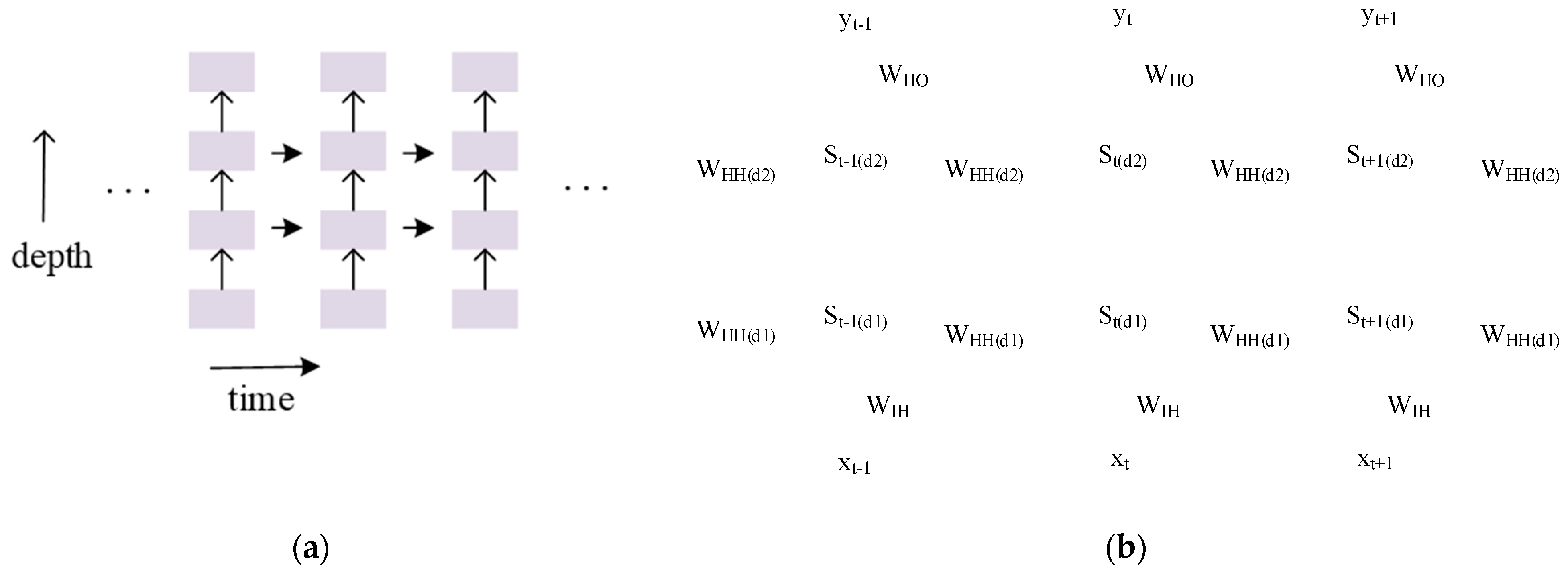
The RNN can form a multi-layer structure, as shown in Figure 4a. According to Formula (4), the smoothed value is another exponential smoothing based on the trend value; therefore, a two-layer RNN structure can be used for fitting. The first-layer $S_t{}_{\left(\mathrm{d}1\right)}$ is calculated based on the first-layer weights and biases and is temporarily stored as the input $x_t{}_{\left(\mathrm{d}2\right)}$ for the second layer. Then, $S_t{}_{\left(\mathrm{d}2\right)}$ is computed based on the second-layer weights and biases, and $S_t{}_{\left(\mathrm{d}1\right)}$ and $S_t{}_{\left(\mathrm{d}2\right)}$ correspond to $S_{t-1}$ of the first and second layers at the second moment, respectively. Therefore, the two-layer RNN structure in Figure 4b represents the current data after second-order exponential smoothing.

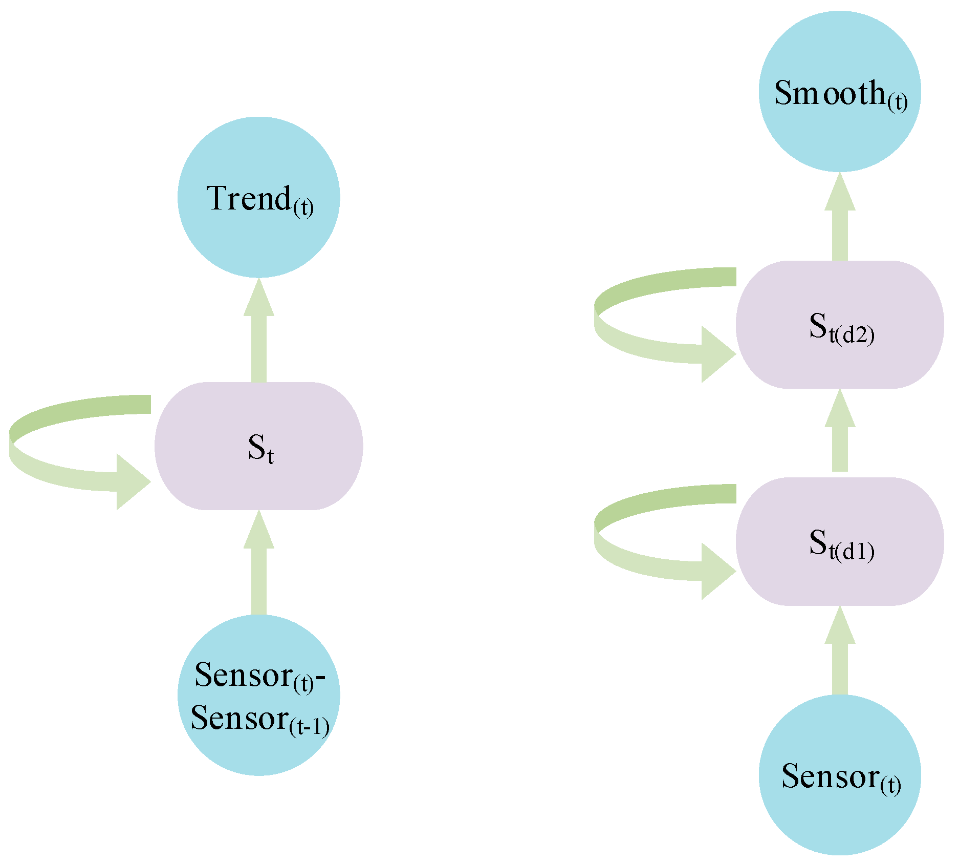
Therefore, the RNN structure for fitting the second-order exponential smoothing is shown in Figure 5. The advantages of this structure are that it does not require prior data preprocessing and, for the difficult parameter selection problem involved in the second-order smoothing, it can be learned through training in the neural network, thereby improving the model’s generalization ability.

The RNN structure in this paper is designed to utilize its memory function for calculating the trend and smooth value of time series data, thereby increasing the interpretability of neural network structure and the universality of the second-order exponential smoothing formula. Therefore, no activation function is needed for nonlinear mapping, simplifying the RNN structure. The exponential smoothing method based on the RNN structure is incorporated into the fully connected neural network. The RNN has two layers with 32 and 16 nodes, respectively, and a single RNN layer with 16 nodes. The outputs of both RNNs are concatenated and fed as input to the three-layer fully connected neural network with eight hidden nodes.

The final output is a binary classification indicating the presence or absence of fire. Since the Sigmoid function has a range of values from 0 to 1 and a characteristic shape that can effectively represent the probability of prediction, it is used as the activation function in the output layer, as shown in Equation (10).

$$Sigmoid\left(x\right)=\frac{1}{1+e^{-x}}$$

(10)

Backpropagation is used in the fully connected layer for nonlinear input–output mapping with the Tanh activation function. The Tanh function has the advantages of being differentiable, nonlinear, and zero-centered. The calculation method is shown in Equation (11).

$$Tanh\left(x\right)=\frac{e^x-e^{-x}}{e^x+e^{-x}}=\frac{1-e^{-2x}}{1+e^{-2x}}=2Sigmoid\left(2x\right)-1$$

(11)

3. Dataset and Training Method

The dataset used in this study is derived from the home fire experiments conducted by the National Institute of Standards and Technology (NIST) in the United States [13]. The experiments involved burning various materials indoors and collecting sensor data at different stages of the fire, including before ignition, early stages, full development, and extinguishment. The performance of several commercially available smoke alarms was also tested. According to statistics, the most frequent types of indoor fires are smoldering upholstered furniture in the living room, flaming upholstered furniture in the living room, smoldering mattresses in the bedroom, and flaming mattresses in the bedroom. Therefore, the dataset selected for this study includes SDC02, SDC05, SDC06, SDC07, SDC08, and SDC11, with a sampling rate of 5 s. These experiments covered the above types of fires and were all conducted in an 85-square-meter manufactured home with a layout similar to most residential buildings.

Table 2. The NIST dataset selected for training.

Dataset	Location of the Fire	Ignition Source	Type of Fire	Amount of Data
SDC02	Living Room	Chair	Flame	313
SDC05	Bedroom	Mattress	Flame	196
SDC06	Bedroom	Mattress	Smoldering	1220
SDC07	Bedroom	Mattress	Flame	170
SDC08	Bedroom	Mattress	Smoldering	1928
SDC11	Living Room	Chair	Smoldering	3543
Total				7370

provides specific information on the selected training datasets.

In the research field of multi-sensor home fire recognition algorithms, selecting appropriate sensor parameters is crucial for improving the sensitivity and anti-interference of fire detection. Experimental studies conducted by the Department of Fire Protection Engineering at the University of Maryland indicate that a combination of temperature rise, CO, and smoke sensors is one of the best choices [14]. Moreover, from the perspective of practical feasibility and cost, there are already examples of fire alarm devices that incorporate these three sensors in the market, such as the smart alarm from Kidde, a manufacturer of fire and safety products. Therefore, this study selects temperature, smoke density, and CO as the fire characteristic parameters collected by sensors. Temperature rise is a fundamental manifestation of combustion, while smoke is generated by all combustible materials during combustion, and its concentration varies depending on the burning material and oxygen content. Compared with smoke, CO is generated earlier, ranging from several tens of minutes to a few hours after the start of the fire. Under normal conditions, the concentration of CO in the air is low, making it a unique marker of fire. Unlike H₂O, O₂, and CO₂, which are not easily affected by the environment and human activities, even in the kitchen environment during cooking, the CO concentration is generally below 20 ppm. CO is suitable for early fire detection and is less likely to produce false alarms.

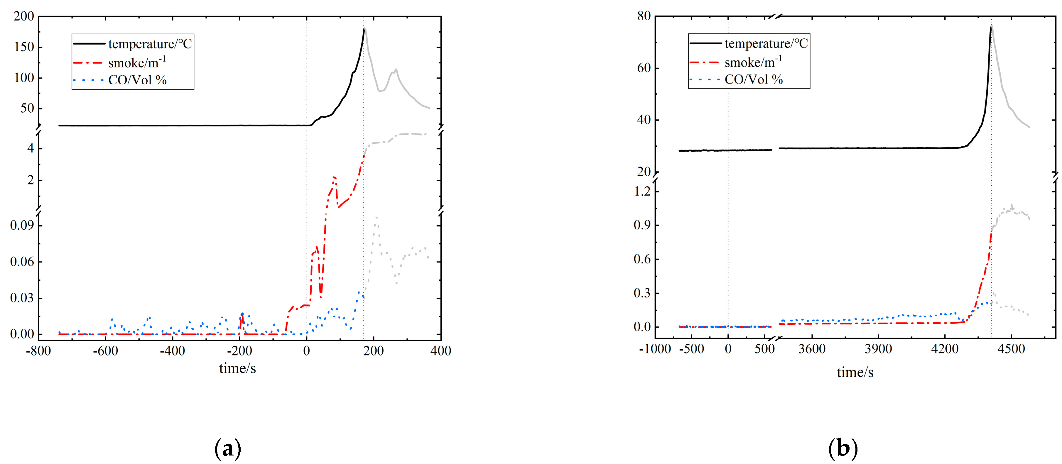
Taking the example of a mattress burning with flame in the bedroom and a chair smoldering in the living room, the sensor data of the three parameters are shown in Figure 6. Before the fire, the values of all parameters in the environment were relatively stable. After ignition at time 0, the sensor data started to fluctuate. As the fire spread to various objects in the house and was affected by ventilation and other environmental factors, the fire intensity gradually decreased, and the sensor data gradually returned to normal. The smoldering fire developed much more slowly than the open flame, and the CO parameter showed the first fluctuations, confirming our decision to include CO as the fire characteristic parameter. Our goal in this study is to develop an algorithm that can accurately identify the occurrence of fire in emergencies. Therefore, we only need to use the data information before the peak of the fire development, as data indicated before the gray curve in Figure 6.

The original sensor time series data were preprocessed by forming a new dataset consisting of tuples with three time points. As the sensor data had different dimensions, it was normalized to values between 0 and 1 for use during neural network training. The dataset was then split into training, validation, and testing sets in the ratios of 0.7, 0.15, and 0.15, respectively. The proposed algorithm flow and related parameters are shown in Figure 7.

The algorithm is trained using the backpropagation method and the Adam optimizer, which combines momentum and adaptive learning rate methods to help the neural network converge quickly. The gradient of each parameter is calculated according to the loss function, and the gradient descent optimization algorithm is used in backpropagation to update the parameters and minimize the loss value. The loss function of the neural network is used to measure the difference between the neural network output and the target output. In this paper, the data label indicates whether a fire has occurred, and the binary cross-entropy loss function can effectively measure the match between the classification probability and the true label. The calculation method of binary cross-entropy is shown in Formula (12), where M is the number of training sets, $y_m$ is the label of training data m, $x_m$ is the training data m, and $h_{\theta }$ is the neural network model with weight $\theta$.

$$J_{bce}=-\frac{1}{M}{\displaystyle \sum }_{m=1}^M\left[y_m\times \log \left(h_{\theta }\left(x_m\right)\right)+\left(1-y_m\right)\times \log \left(1-h_{\theta }\left(x_m\right)\right)\right]$$

(12)

4. Assessment Method

This study mainly compared several algorithms that consider the development trend of fires, including the algorithm that introduces the development trend of fires from existing literature in Section 3 and the algorithm proposed in this paper that introduces the second-order exponential smoothing method. The following algorithms were selected for comparison.

The first algorithm compared in this paper is a neural network, as shown in Figure 1, where the sensor data are only processed with a simple average filter (BPNN).

The second algorithm compared in this paper is the one proposed in reference [4] (TPNN).

The third algorithm compared in this paper is the “Improved kendall-τ NN” proposed in reference [5], which extracts the fire development trend using an improved Kendall-τ formula from sensor data.

A neural network directly incorporating the second-order exponential smoothing formula, where the smoothing parameters α and β are set to empirical values (α = 0.5, β = 0.5) and fitted using the TRF and Dogbox methods (ES-formula NN).

A neural network model with an RNN structure fitted to the second-order exponential smoothing formula proposed in this paper (ES-RNN).

Classification in fire detection is a binary model where a positive label is assigned to the result when a fire is detected, and a negative label is assigned when there is no fire. Therefore, the neural network classification results can be divided into the following situations:

• True positive (TP) refers to the samples that are correctly predicted as positive labels.
• False negative (FN) refers to the samples that are incorrectly predicted as negative labels.
• True negative (TN) refers to the samples that are correctly predicted as negative labels.
• False positive (FP) refers to the samples that are incorrectly predicted as positive labels.

To evaluate the performance of the algorithm models and determine whether they are suitable for indoor fire detection, we have selected the following evaluation metrics based on specific data to support the rationality of the algorithms.

Accuracy is a metric that measures the proportion of correctly classified samples in the total number of samples. It is defined as shown in Equation (13).

$$\mathrm{accuracy}=\frac{\mathrm{TP}+\mathrm{TN}}{\mathrm{TP}+\mathrm{TN}+\mathrm{FP}+\mathrm{FN}}$$

(13)

Precision measures the proportion of true positive cases among all positive cases identified by the model. It is calculated as shown in Equation (14). Compared to accuracy, precision focuses more on positive samples, that is, examining whether there are any misclassifications when judging the results as fire incidents.

$$\mathrm{precision}=\frac{\mathrm{TP}}{\mathrm{TP}+\mathrm{FP}}$$

(14)

Recall represents the ability of an algorithm to identify positive cases. The formula is shown as (15). In this paper, positive cases refer to fire incidents, and recall represents the ability to identify fire incidents.

$$\mathrm{recall}=\frac{\mathrm{TP}}{\mathrm{TP}+\mathrm{FN}}$$

(15)

The F1 score, with a range of values between 0 and 1, is the harmonic mean of precision and recall. It provides a more comprehensive evaluation than precision and recall alone when either of them is not sufficient to fully capture the model’s performance [15]. In this paper, we also use the F1 score to evaluate the model’s ability to identify fire incidents, with fire incidents being considered positive. The formula is shown in Equation (16):

$$\mathrm{F}1 \mathrm{score}=2·\frac{\mathrm{precision}·\mathrm{recall}}{\mathrm{precision}+\mathrm{recall}}$$

(16)

The receiver operating characteristic (ROC) curve is plotted based on two metrics: true positive rate and false positive rate, as shown in Formulas (17) and (18):

$$\mathrm{TPR}=\mathrm{sensitive}=\frac{\mathrm{TP}}{\mathrm{TP}+\mathrm{FN}}$$

(17)

$$\mathrm{FPR}=1-\mathrm{specificity}=\frac{\mathrm{FP}}{\mathrm{FP}+\mathrm{TN}}$$

(18)

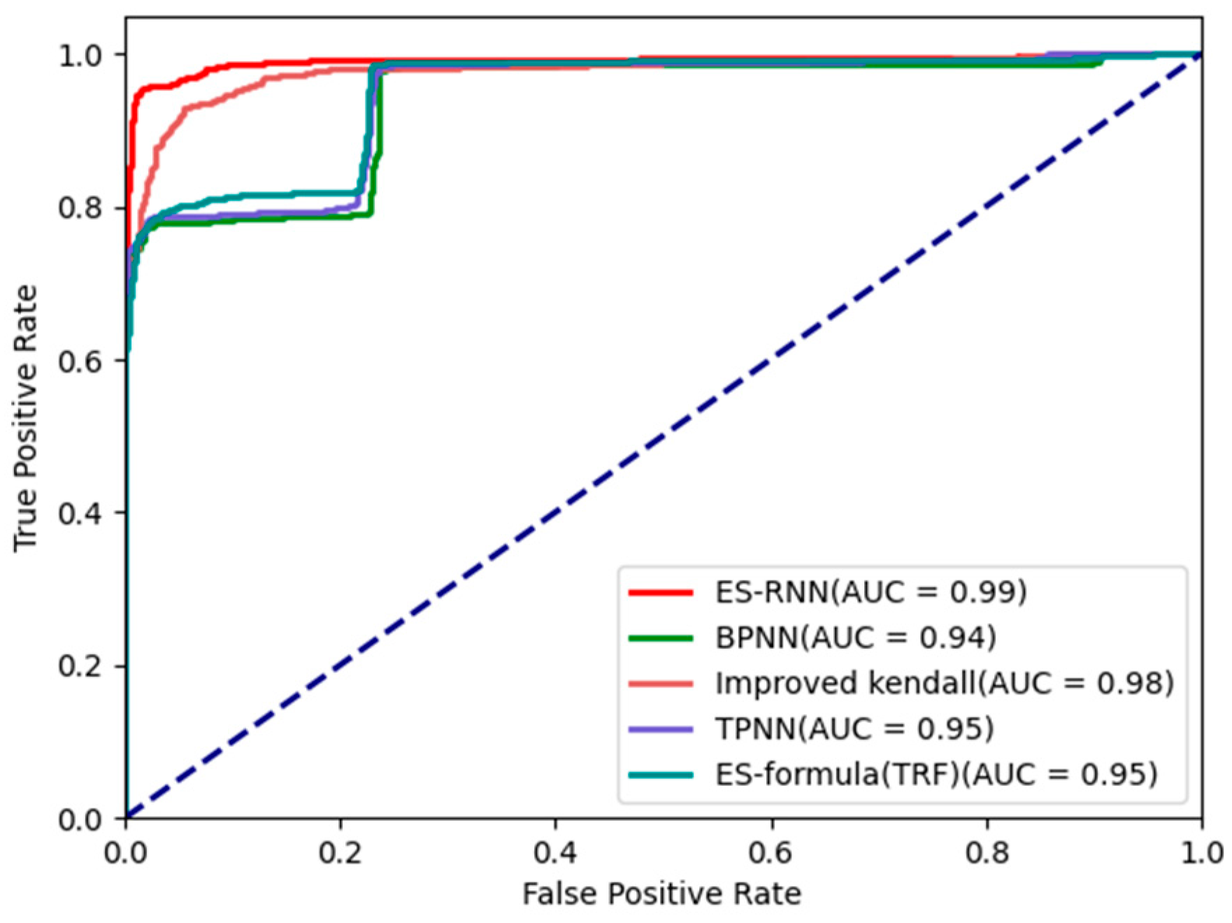
Neither TPR nor FPR is affected by class imbalance. The FPR represents the degree of false reporting of fires, while the TPR represents the coverage ratio of the classification results as having fires. Therefore, the lower the FPR and the higher the TPR, the better the performance of the model. Area under ROC curve (AUC) is a comprehensive measure of the overall performance of the model corresponding to the classification threshold traversed. The area below the diagonal line represents random classification. The steeper the ROC curve and the larger the AUC, the better the model performance.

The Matthews Correlation Coefficient (MCC) calculates the Pearson product–moment correlation coefficient between the actual and predicted values using a contingency table and is not affected by imbalanced datasets [16]. The MCC calculation is shown in Equation (19):

$$\mathrm{MCC}=\frac{\mathrm{TP}·\mathrm{TN}-\mathrm{FP}·\mathrm{FN}}{\sqrt{\left(\mathrm{TP}+\mathrm{FP}\right)·\left(\mathrm{TP}+\mathrm{FN}\right)·\left(\mathrm{TN}+\mathrm{FP}\right)·\left(\mathrm{TN}+\mathrm{FN}\right)}}$$

(19)

The MCC ranges from −1 to +1, where a perfect classifier has an MCC of 1, an MCC of 0 corresponds to random classification, and a completely inverted binary classification results in an MCC of −1 [17].

5. Results and Discussion

5.1. Performance Analysis of Algorithms

The evaluation metrics for fire detection performance on the time-split dataset using different algorithms are presented in

Table 3. Comparison of performance metrics among different algorithms.

	Accuracy	Precision	Recall	F1- Score	FPR	MCC	AUC
ES-RNN	0.98	0.96	0.98	0.97	0.03	0.95	0.99
BPNN	0.90	0.96	0.77	0.86	0.02	0.79	0.94
TPNN	0.90	0.96	0.78	0.86	0.02	0.79	0.95
$\mathrm{Improved} \mathrm{kendall} -\mathsf{\tau }$ NN	0.94	0.92	0.93	0.92	0.06	0.87	0.98
$\mathrm{ES}-\mathrm{formula} \mathrm{NN} \left(\alpha =0.5,\beta =0.5\right)$	0.89	0.93	0.79	0.86	0.04	0.78	0.91
ES-formula NN (TRF Fitting)	0.93	0.88	0.97	0.92	0.09	0.87	0.95
ES-formula NN (Dogbox Fitting)	0.92	0.86	0.97	0.91	0.11	0.84	0.95

.

Based on Table 3, the trend-based model is more ideal than the BPNN model, which only performs data smoothing. The TPNN model only shows a slight improvement in recall rate and AUC metrics, so it is not the best trend optimization method for the selected dataset. By introducing the improved Kendall-τ formula, the neural network has shown improvements in accuracy, recall rate, F1 score, MCC, and AUC, indicating an overall enhancement in the classification ability of the model.

However, the decrease in precision and the increase in FPR suggest that the model’s false positive rate has also increased. Using the formula of second-order exponential smoothing alone with uncertain parameters cannot guarantee the model’s performance improvement, such as α = 0.2 and β = 0.8. However, the model’s recognition ability can be improved by selecting suitable parameters. To simultaneously improve recognition accuracy and minimize the possibility of false alarms, the method of using RNN to complete the second-order exponential smoothing is more suitable for practical requirements. As shown in Table 1, the ES-RNN model has achieved the maximum F1 score and MCC, indicating that the performance of the binary classifier implemented in this way is among the best in the compared models.

In the method of introducing the second-order exponential smoothing, Table 3 compares the performance of four models formed by determining smoothing parameters empirically, defining smoothing parameters through TRF and Dogbox algorithms, and fitting smoothing parameters through RNN. Due to the uncertainty of the parameters, it cannot be guaranteed that the performance of the model will be improved. For example, the algorithm with α = 0.5 and β = 0.5 selected according to empirical values does not perform well in terms of recognition accuracy. However, if suitable parameters are chosen, the recognition capability of the model can be improved. Here, the parameters fitted by TRF and Dogbox algorithms are, respectively, substituted into the quadratic exponential smoothing formula to form a neural network algorithm, and the model is tested with the dataset. It can be seen that the accuracy of the model fitted by the TRF algorithm can be improved to 93%, which has a better performance than that of Dogbox.

In order to simultaneously improve the recognition accuracy and reduce the false alarm rate, this paper adopts a method of using RNN to implement quadratic exponential smoothing, that is, ES-RNN. As shown in Table 3, the F1 score and MCC of ES-RNN are the highest, indicating that this algorithm performs better than other models, and the false alarm rate of this algorithm is also relatively low (FPR = 3%). The ROC curve and AUC results shown in Figure 8 also confirm the best performance of the ES-RNN model.

At the same time, the false positive rate is also maintained at a relatively low level. Figure 8 shows the ROC curve and AUC results, which further confirm the superiority of this model. After the output layer’s sigmoid function, the model’s output result is a decimal between 0 and 1, and a threshold is used to determine the final classification. The point on the ROC curve closest to the top left corner, with the largest TPR and the smallest FPR, represents the best threshold. For ES-RNN, the optimal threshold is 0.553.

5.2. Alarm Time Test

To ensure the generalizability of the ES-RNN algorithm to different residences, a validation of alarm times was conducted in a new house. The data were still obtained from the NIST experiment, which helped to exclude the effects of irrelevant factors such as differences in sensor model and extraction standards. The test location was a two-story brick house with three bedrooms and an area of 139 square meters. We selected the datasets listed in

Table 4. Comparison results of alarm time between traditional sensors and ES-RNN model.

Num	Type of Fire	Alarm Time of Smoke Alarms (Photoelectric and Ionization) [s]	Alarm Time of CO Alarms [s]	Alarm Time of the Proposed Model [s]
I	Flaming Chair in Living Room	116–176	202–282	96
II	Flaming Chair in Living Room	126–238	254–302	100
III	Flaming Mattress in Bedroom	32–108	154–214	46
IV	Flaming Mattress in Bedroom (Burn Room Door Closed)	160–454	264–2044	180
V	Smoldering Chair in Living Room	1162–4902	744–4896	353
VI	Smoldering Chair in Living Room (Air Conditioning on Second Floor)	1156–4252	2030–4248	3541
VII	Smoldering Mattress in Bedroom	Alarm not Reached	Alarm not Reached	Not Sure
VIII	Fully involved living room	76–232	-	230

for validation, using only the data before the fire reached its peak. The alarm times from conventional fire alarms, including smoke alarms (photoelectric/ionization sensors) and CO alarms, were used as a reference, as they are actual products in use. Due to differences in their models and threshold configurations, the table presents the range of alarm times for each corresponding alarm.

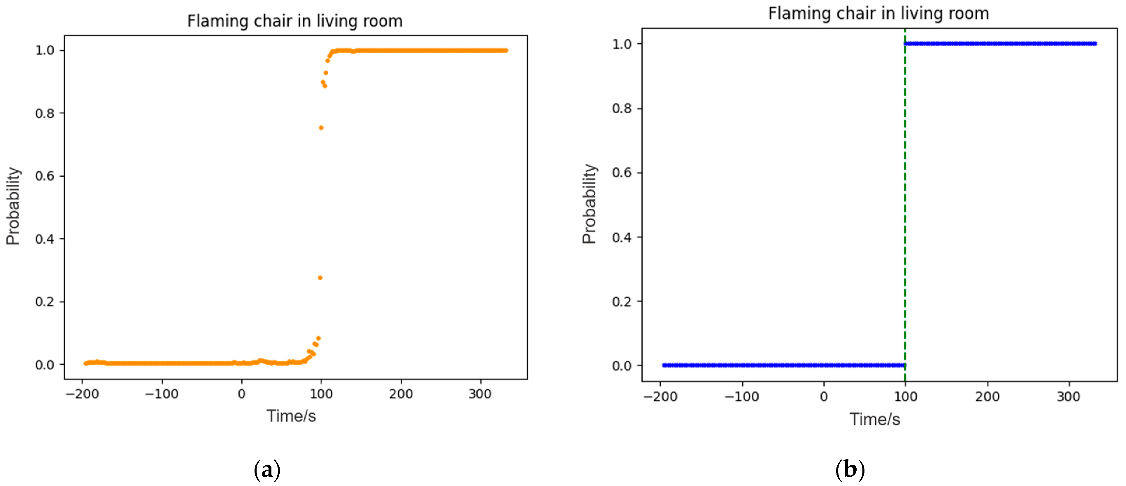
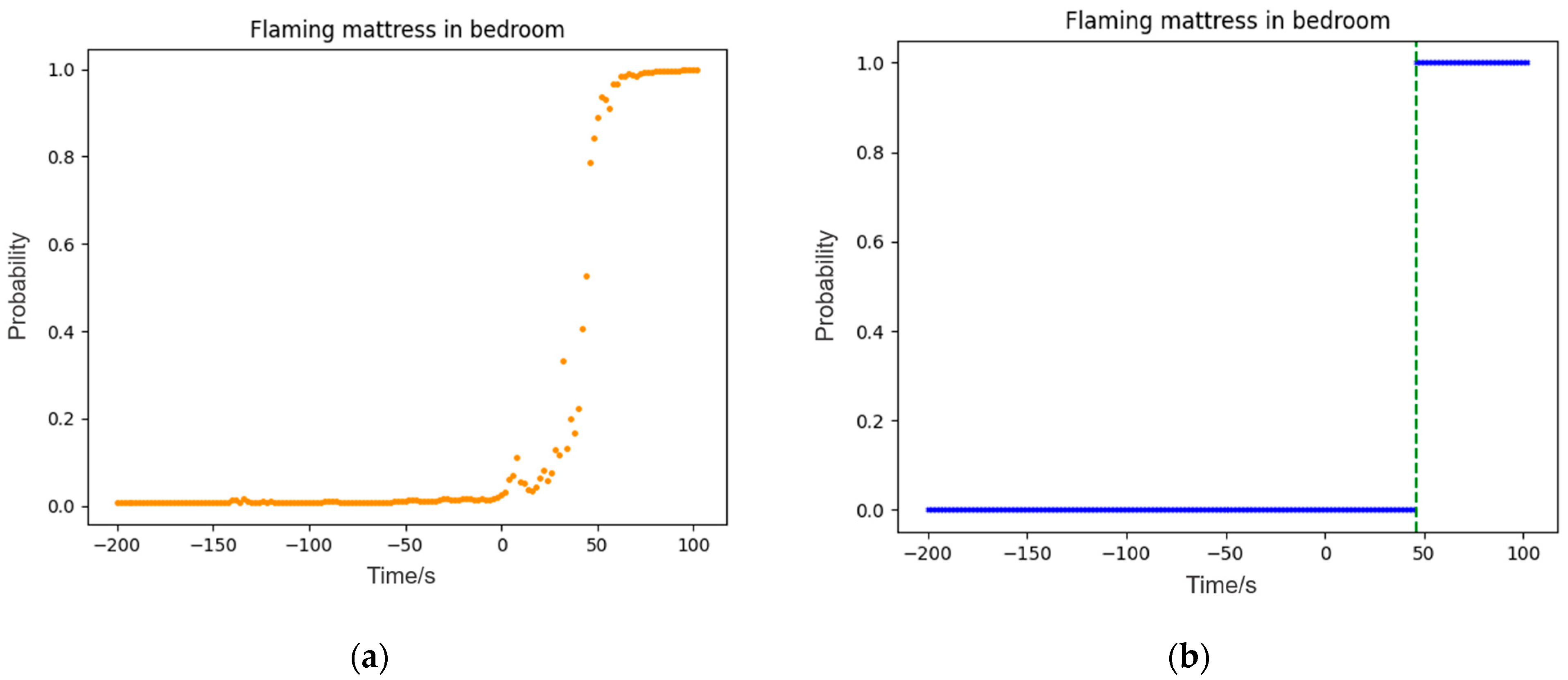
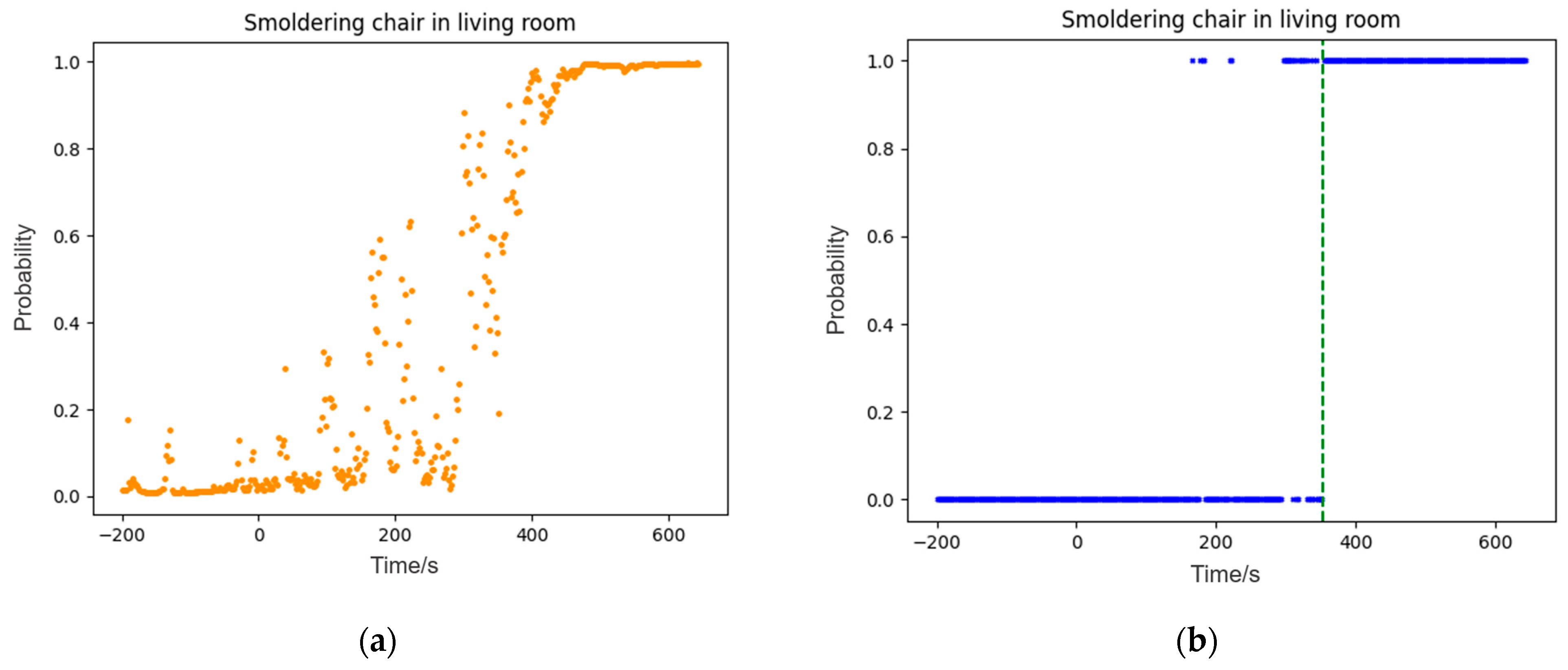
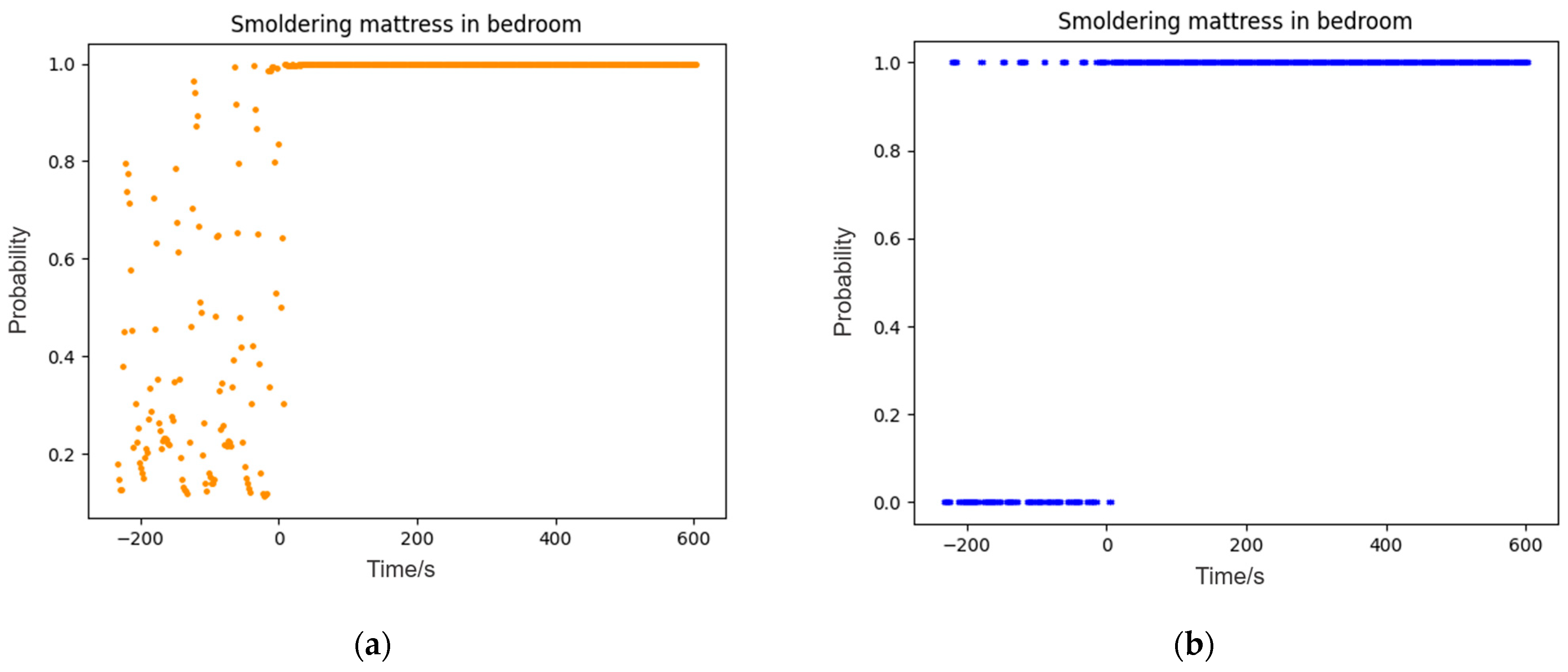
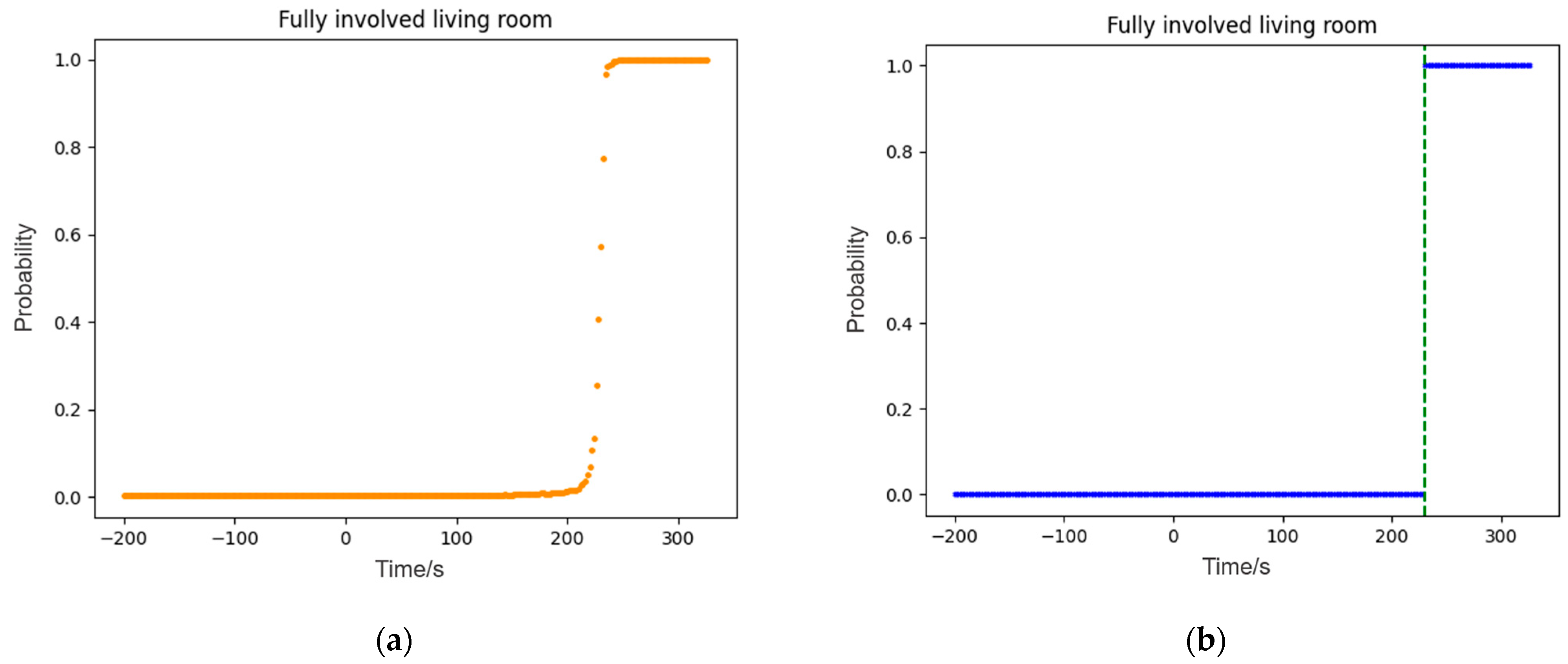
Figure 9, Figure 10, Figure 11, Figure 12, Figure 13, Figure 14, Figure 15 and Figure 16 display the output of the model after passing through the sigmoid function, shown in (a) as decimal numbers between 0 and 1. The final result is shown in (b), where a value of 1 indicates the presence of a fire, while a value of 0 indicates no fire. The dashed line indicates the alarm time after the system reaches stability.

Figure 9 and Figure 10 both depict a scenario where a chair in the living room is ignited. The experimental results obtained using the smoke detectors (photoelectric/ionization) and CO detectors reveal the instability of the alarm time in this environment. In some cases, the CO alarm can generate an alarm signal quickly, but only if its sensitivity is set at a high level, according to the full report of this NIST experiment. The algorithm proposed in this paper achieves more consistent alarm times in this type of fire and ignition source and is earlier than most traditional alarms.

Compared with Experiment I, Experiment II has a longer fire growth period according to the official NIST experiment report. Therefore, the alarm time of Experiment II is relatively delayed compared to Experiment I, as observed from the alarm time of traditional alarm devices in their most sensitive state (i.e., fastest alarm). Specifically, the alarm time of the photoelectric and ion sensors lags by 10 s, while the alarm time of the CO sensor lags by 52 s. In contrast, the alarm time of the proposed algorithm lags only by 4 s. Consequently, the proposed algorithm can identify fires more sensitively and timely.

Figure 11 presents the detection results from Experiment III, where a mattress in the bedroom was ignited. In contrast to Experiments I and II, the proposed algorithm in this paper showed an earlier detection result, with about 50 s earlier identification of this fire situation. This is related to the choice of the chair with low foam content used in the open flame experiment, as well as the location of the fire source. The alarm time provided by the traditional alarms also confirmed that the fire in this experiment indeed developed more quickly and visibly. However, the algorithm proposed in this paper still demonstrated the advantage of timely alarm.

The results of Experiment IV, shown in Figure 12, indicate that the alarm time of our model, as well as the other two traditional alarm devices, is delayed. This is because the burning process is restricted in a closed-door room, which slows down the spread of the fire. Under such conditions, the alarm time of our algorithm remains relatively early.

Compared to flaming fires, smoldering fires usually take longer to generate enough smoke to trigger an alarm. According to the National Fire Protection Association (NFPA), the alarm time for smoldering fires should be less than or equal to 60 min. As shown in Figure 13, which presents the results of Experiment V, our model judged the occurrence of fire completely after 353 s in this smoldering fire experiment. During a small period before 353 s, the output fluctuated between fire and no fire. The alarm time is completely within the prescribed range and has a significant time advantage compared to traditional alarms.

In comparison to Experiment V, Experiment VI had an air conditioner turned on in the second room, causing changes in environmental factors such as temperature and air flow. As shown in Figure 14, the alarm time of our model was significantly delayed, indicating that these environmental factors had an impact on the model and further optimization is needed in the future.

The alarm time of our model was not provided in Table 4, as shown in Figure 15, because the model incorrectly detected a fire before the start of the experiment. Although the model correctly identified the presence of a fire after the start of the experiment, it is unclear whether the initial detection was due to environmental factors or an actual fire. This is a model defect that needs to be addressed in the future as it is caused by the influence of the environment on the model.

The results of Experiment VIII are shown in Figure 16, where various household items in the living room were ignited. Our proposed model provided the recognition of the fire within a comparable time frame to that of traditional alarms.

Overall, the algorithm proposed in this paper can timely recognize most fire situations. However, in some cases, the model’s performance is affected by environmental factors, which requires further research with more real data.

6. Conclusions and Future Work

This paper focuses on the research of advanced information fusion technology for indoor fire detection. In view of the shortcomings of existing fire alarm models based on information fusion, this study innovatively proposes a fire alarm algorithm focusing on the time series characteristics. We introduce a second-order exponential smoothing method to simplify the drawbacks of data preprocessing using moving averages and obtain both smooth and trend data. An RNN structure is used to fit the second-order exponential smoothing formula and solve the problem of difficult parameter selection, improving the algorithm’s generalization ability. This method enhances the adaptability of the second-order exponential smoothing method to different fire data. The proposed ES-RNN algorithm achieves an accuracy of up to 98%, with F1-score and Matthews correlation coefficient reaching 0.97 and 0.95, respectively, demonstrating its superiority in classifying positive and negative samples. This paper also verifies the timely alarm requirement of the algorithm, which has certain advantages compared to traditional alarms.

To further improve the practicality of this fire alarm system, future work should focus on optimizing it for a wider range of fire data and reducing the interference of environmental factors on alarm performance. In addition, hardware implementation of the entire system should be conducted and validated in real-world scenarios.

References

1. Yancheng, C.; Liheng, W. Design and Implementation of Fire Monitoring and Warning User Terminal System. In Proceedings of the 2022 International Conference on Artificial Intelligence and Computer Information Technology (AICIT), Yichang, China, 16–18 September 2022; pp. 1–5. [Google Scholar]
2. Okayama, Y. A primitive study of a fire detection method controlled by artificial neural net. Fire Saf. J. 1991, 17, 535–553. [Google Scholar] [CrossRef]
3. Chen, J.; Fu, J.Q. Fire Alarm System Based on Multi-Sensor Bayes Network. In Proceedings of the 2012 International Workshop on Information and Electronics Engineering, Harbin, China, 10–11 March 2012; pp. 2551–2555. [Google Scholar]
4. Nakıp, M.; Güzeliş, C. Multi-Sensor Fire Detector based on Trend Predictive Neural Network. In Proceedings of the 2019 11th International Conference on Electrical and Electronics Engineering (ELECO), Bursa, Turkey, 28–30 November 2019; pp. 600–604. [Google Scholar]
5. Wu, L.; Chen, L.; Hao, X. Multi-Sensor Data Fusion Algorithm for Indoor Fire Early Warning Based on BP Neural Network. Information 2021, 12, 59. [Google Scholar] [CrossRef]
6. Wu, L.B.; Yuan, H. Fire Detection and Control Engineering; University of Science and Technology of China Press: Hefei, China, 2013. [Google Scholar]
7. Hamed, K. Exact distribution of the Mann–Kendall trend test statistic for persistent data. J. Hydrol. 2009, 365, 86–94. [Google Scholar] [CrossRef]
8. Brown, R.G.; Meyer, R.F.; D’Esopo, D.A. The Fundamental Theorem of Exponential Smoothing. Oper. Res. 1961, 9, 673–687. [Google Scholar] [CrossRef]
9. Li, G.; Cai, Z.; Kang, X.; Wu, Z.; Wang, Y. ESPSA: A prediction-based algorithm for streaming time series segmentation. Expert Syst. Appl. 2014, 41, 6098–6105. [Google Scholar] [CrossRef]
10. Gardner, E.S., Jr. Exponential smoothing: The state of the art. J. Forecast. 1985, 4, 1–28. [Google Scholar] [CrossRef]
11. Wu, L.F.; Liu, S.F.; Yang, Y.J. Grey double exponential smoothing model and its application on pig price forecasting in China. Appl. Soft Comput. 2016, 39, 117–123. [Google Scholar] [CrossRef]
12. Zhang, Y.; Guo, X.; Liu, R.; Zhang, H.B. Research on Network Security Trend Prediction Based on Exponential Smoothing Algorithm. In Proceedings of the 2020 IEEE 11th International Conference on Software Engineering and Service Science (Icsess 2020), Beijing, China, 16–18 October 2020; pp. 507–510. [Google Scholar]
13. Bukowski, R.W.; Peacock, R.D.; Averill, J.D.; Cleary, T.G.; Bryner, T.G.; Walton, W.D.; Reneke, P.A.; Kuligowski, E.D. Performance of Home Smoke Alarms: Analysis of the Response of Several Available Technologies in Residential Fire Settings; Technical Note (NIST TN); National Institute of Standards and Technology: Gaithersburg, MD, USA, 2006; p. 1455. [Google Scholar]
14. Cestari, L.A.; Worrell, C.; Milke, J.A. Advanced fire detection algorithms using data from the home smoke detector project. Fire Saf. J. 2005, 40, 1–28. [Google Scholar] [CrossRef]
15. Parker, C. An Analysis of Performance Measures for Binary Classifiers. In Proceedings of the 2011 IEEE 11th International Conference on Data Mining, Vancouver, BC, Canada, 11–14 December 2011; pp. 517–526. [Google Scholar]
16. Powers, D. Evaluation: From Precision, Recall and F-Factor to ROC, Informedness, Markedness & Correlation. Mach. Learn. Technol. 2008, 2, 2229–3981. [Google Scholar]
17. Chicco, D.; Jurman, G. The advantages of the Matthews correlation coefficient (MCC) over F1 score and accuracy in binary classification evaluation. BMC Genom. 2020, 21, 6. [Google Scholar] [CrossRef] [PubMed]
Figure 1. The structure of information fusion fire warning system.
Information 14 00258 g001
Figure 2. The structure of information fusion fire warning system with trend extraction.
Information 14 00258 g002
Figure 3. Single−layer RNN model architecture.
Information 14 00258 g003
Figure 4. (a) The structure of multi−layer RNN model; (b) two−layer RNN structure used for fitting in second−order exponential smoothing.
Information 14 00258 g004
Figure 5. The structure of RNN fitting second−order exponential smoothing.
Information 14 00258 g005
Figure 6. Example of how sensor data changes during a fire including (a) the sensor data of flaming mattress in bedroom; (b) the sensor data of smoldering chair in living room.
Information 14 00258 g006
Figure 7. Flowchart of ES−RNN algorithm.
Information 14 00258 g007
Figure 8. Comparison of ROC/AUC results among different algorithms.
Information 14 00258 g008
Figure 9. (a) Model output of experiment I; (b) results of alarm time in experiment I.
Information 14 00258 g009
Figure 10. (a) Model output of experiment II; (b) results of alarm time in experiment II.
Information 14 00258 g010
Figure 11. (a) Model output of experiment III; (b) results of alarm time in experiment III.
Information 14 00258 g011
Figure 12. (a) Model output of experiment IV; (b) results of alarm time in experiment IV.
Information 14 00258 g012
Figure 13. (a) Model output of experiment V; (b) results of alarm time in experiment V.
Information 14 00258 g013
Figure 14. (a) Model output of experiment VI; (b) results of alarm time in experiment VI.
Information 14 00258 g014
Figure 15. (a) Model output of experiment VII; (b) results of alarm time in experiment VII.
Information 14 00258 g015
Figure 16. (a) Model output of experiment VIII; (b) results of alarm time in experiment VIII.
Information 14 00258 g016