Article

A Deep Learning Model for Ship Trajectory Prediction Using Automatic Identification System (AIS) Data

Merchant Marine College, Shanghai Maritime University, Shanghai 201306, China
*
Author to whom correspondence should be addressed.
Information 2023, 14(4), 212; https://doi.org/10.3390/info14040212
Submission received: 15 December 2022 / Revised: 13 March 2023 / Accepted: 16 March 2023 / Published: 30 March 2023

Abstract

:
The rapid growth of ship traffic leads to traffic congestion, which causes maritime accidents. Accurate ship trajectory prediction can improve the efficiency of navigation and maritime traffic safety. Previous studies have focused on developing a ship trajectory prediction model using a deep learning approach, such as a long short-term memory (LSTM) network. However, a convolutional neural network (CNN) has rarely been applied to extract the potential correlation among different variables (e.g., longitude, latitude, speed, course over ground, etc.). Therefore, this study proposes a deep-learning-based ship trajectory prediction model (namely, CNN-LSTM-SE) that considers the potential correlation of variables and temporal characteristics. This model integrates a CNN module, an LSTM module and a squeeze-and-excitation (SE) module. The CNN module is utilized to extract data on the relationship among different variables (e.g., longitude, latitude, speed and course over ground), the LSTM module is applied to capture temporal dependencies, and the SE module is introduced to adaptively adjust the importance of channel features and focus on the more significant ones. Comparison experiments of two cargo ships at a time interval of 10 s show that the proposed CNN-LSTM-SE model can obtain the best prediction performance compared with other models on evaluation indexes of average root mean squared error (ARMSE), average mean absolute percentage error (AMAPE), average Euclidean distance (AED), average ground distance (AGD) and Fréchet distance (FD).

1. Introduction

Ships, as the main carriers of global trade, play an increasingly important role in the rapid development of technology and economic trade [1]. At present, the number of ships used in China is growing significantly [2]. As a primary means of maritime transportation, ships have made important contributions to social progress and economic development [3]. However, with the increasing number of ships, marine traffic is becoming more crowded [4,5]. Maritime traffic accidents show a rising trend; therefore, ensuring maritime traffic safety is a challenge. Port traffic organization, maritime search and rescue, customs anti-smuggling and other activities make it necessary to predict ship navigation trajectories in the near future to ensure orderly and safe passage among ships. Therefore, accurate and effective ship trajectory prediction is essential to enhance maritime safety.
The automatic identification system (AIS) is an important source of data for maritime traffic analysis (e.g., trajectory prediction, collision avoidance analysis, abnormal behavior detection, etc.) [6,7,8]. AIS is a digital navigation system between ship and shore and between ship and ship. According to international maritime organization (IMO) conventions, international merchant ships (e.g., tankers, container ships, etc.) with a deadweight of more than 300 tons and ships with passengers are required to carry AIS equipment and keep it switched on [9]. AIS data provide an abundance of real-time information on ship navigation, which is conducive to the real-time supervision of ships by relevant departments at sea, improves the efficiency of ship navigation and ensures navigation safety [10].
With the development of deep learning technology, scholars have increasingly focused on obtaining a high-accuracy ship trajectory prediction using deep learning models [11,12,13]. Chen et al. [14] applied a Bi-LSTM model which demonstrated a satisfactory accuracy not only on single vessel trajectory prediction but also on multi-vessel trajectory prediction. Ship navigation surroundings such as waves, wind and buoys may interfere with ship maneuvering operations and lead to uncertainty in a ship’s trajectory that can affect predictive performance. Qian et al. [15] used a genetic algorithm (GA) to optimize the hyperparameters of LSTM and further proposed a GA-LSTM model to predict inland ship trajectories in real time. In long-distance ship position prediction, the calculation cost of the proposed model would be relatively high, and it would be impractical in collision avoidance maneuvering. Liu et al. [16] proposed a trajectory prediction model based on adaptive chaos differential evolution algorithm (ACDE) and support vector regression (SVR) and combined the proposed model with abundant ship AIS data to solve the ship trajectory prediction problem. However, the proposed model was an offline model and could not be modified once the model has been trained. Zhang et al. [17] used multi-scale convolutional neural networks to extract specific features from multiple input data and proposed a method for predicting ship trajectory that incorporates a gated recurrent unit and attention mechanism (GRU-AM) and an autoregression (AR) model, which combines linear and non-linear models and improves the prediction accuracy of the model. However, the calculation cost of the model was relatively high. Volkova et al. [18] constructed a two-layer neural network to predict ship trajectory and used the idea of gradient descent to estimate movement trends. Park et al. [19] performed spectral clustering of AIS data to obtain ship trajectories with similarities and developed spectrally clustered AIS data using a Bi-LSTM model to predict the future ship trajectory. Suo et al. [20] first performed a cluster analysis and similarity measurement on ship trajectory data in order to avoid errors during data transmission, and then proposed a prediction model based on gated recurrent units (GRU). Bao et al. [21] proposed a deep learning model that used a multi-head attention (MHA) mechanism to calculate the correlation between each parameter to further accurately predict ship trajectory using the bidirectional gate recurrent unit (BiGRU) model. The trajectory of a ship was uncertain and subject to spatial information from other ships and bad weather, which was not considered in the literature [18,19,20,21]. Sørensen et al. [22] used a trajectory prediction model with Bi-LSTM architecture to predict a probabilistic future location as opposed to a deterministic location. The same past trajectory could result in several probable future trajectories. Zhao et al. [23] proposed a novel ensemble machine learning model to predict ship trajectory variation with the help of the EMD and ANN models. The proposed framework would rely on the historical trajectory samples. Gao et al. [24] proposed the uncertainty modelling method for the future trajectory of a ship based on multivariate Gaussian assumptions and Gaussian processes. The proposed model calculations were complex. Zheng et al. [25] proposed the hybrid model, which combines the Sine chaos mapping to improve the population quality of SSA and the optimization of the SSA-BP neural network. Ship performance and spatial characteristics were not fully considered in the proposed model. The above literature provides many ideas and methods for ship tracking prediction model design and represents the most significant prior research relevant to this paper. However, the above literature does not take into account the different effects of various data features on the trajectory prediction results, and the key data features that have a high impact on these results should be identified.
The attention mechanism has been widely used in the field of traffic flow prediction, and important breakthroughs have been made. Wang et al. [26] used an attention mechanism to filter out useless feature information to improve the accuracy of traffic flow prediction. Zhao et al. [27] proposed pyramid feature attention networks, which are optimized using channel attention to retain more structural information. Wang et al. [28] proposed a traffic flow prediction model based on deep learning and an attention mechanism to extract spatial and temporal features, which was well suited to the task of short-term traffic flow prediction.
This paper proposes a ship trajectory prediction model based on a convolutional neural network, long short-term memory and squeeze-and-excitation (SE) network (the CNN-LSTM-SE model). The proposed model considers the superiority of CNN in extracting the correlation of data features and the superiority of the LSTM model in handling time series data. It then applies the SE network to the field of ship trajectory prediction by focusing on the most important data features. The CNN-LSTM model, CNN model and LSTM model are selected as the comparative models, and ship AIS data are selected for example analysis. The results of the comparative experiments show that the proposed method has a better predictive performance. The CNN-LSTM-SE model obtained better prediction accuracy than other models (i.e., CNN-LSTM model, CNN model, and LSTM model) from the perspective of ARMSE, AMAPE, AED, AGD, and FD. The rest of this paper is organized as follows. Section 2 describes the methodology used in the paper. Section 3 contains experiments and analysis. Finally, Section 4 concludes the paper.

2. Methodology

2.1. Research Framework

In this paper, based on AIS dynamic data, the CNN-LSTM-SE model is used to predict the future position of a ship. Figure 1 illustrates the three components of the research framework: data preprocessing, model construction and model validation. Firstly, the collected ship AIS data is preprocessed, including abnormal data processing, missing value processing and data normalization. Then, a deep-learning-based ship trajectory prediction model is proposed. Longitude, latitude, speed and course over ground are considered as the input, and the output is the location of the ship (i.e., longitude and latitude). Finally, to verify the prediction performance of the proposed model, comparison experiments are conducted with the CNN-LSTM model, CNN model and LSTM model at different time intervals (10 s, 30 s, and 1 min).

2.2. Data Preprocessing

Due to unstable signal transmission rates and data transmission congestion, raw AIS data can suffer from data anomalies. There are many methods for cleaning outliers. Common methods include simple statistical analysis, cluster analysis, box plot analysis and the three sigma guidelines. In this paper, a simple statistical analysis is used, with the upper and lower normal limits of the data in the area used as the prescribed boundary for outliers. Values beyond this boundary are considered outliers and removed.
The time interval of each obtained time point is unequal due to the different sending times of AIS messages of ships. In order to ensure the completeness and accuracy of the ship trajectory, missing data need to be completed according to the time interval sampled. Common interpolation methods are linear interpolation, mean interpolation, Lagrange interpolation and spline interpolation [29,30]. In this paper, spline interpolation is employed for longitude and latitude, and linear interpolation is used for speed and course over ground.
Spline interpolation is a segmental interpolation method consisting of a polynomial function. The neighboring data points before and after the missing values are constructed as data intervals, and the interval [ x i , x i + 1 ] is noted as the i-th interval. For each interval, a k-order polynomial spline function f(x) is constructed. Its order in each interval is no greater than k and has continuous derivatives of the order k − 1.
f ( x ) = φ 0 + φ 1 x 1 + + φ k x k
where φ i is a function parameter.
The linear interpolation method assumes that the ship is sailing in an approximately straight line, and it estimates the missing data using the two closest sets of data before and after the missing point. Assuming that ( t i ,   P i ) are the missing data and the two trajectory points before and after this point are ( t m ,   P m ) and ( t n ,   P n ) , the data for the inserted trajectory point can be calculated by the following formula.
P i = P n + P n P m t n t m ( t i t m )
Because the ship’s longitude and latitude are relatively constant within a short period of time, this model adopts the spline interpolation method to determine the ship’s longitude and latitude data. For the missing values of speed and course over ground, there is usually a less rapid change of course when the ship is sailing. Since the ship’s speed and course over ground data are relatively smooth, this paper uses linear interpolation [14,21].
Different dimensionality of data can affect the prediction performance of the model. Therefore, to eliminate the dimensionality among the different data and to improve the convergence speed of the model during training, it is necessary to normalize the data. The normalization method chosen to convert the data in this model is min–max normalization, which normalizes the original data values to the range [0, 1] [31].
a * = a m i n m a x m i n
where max is the maximum value of a, min is the minimum value of a, a * is the normalized data and a is the original data.

2.3. Ship Trajectory Prediction Based on CNN-LSTM-SE

2.3.1. Convolutional Neural Network (CNN)

Convolutional neural networks (CNNs) evolved from the multilayer perceptron and have the features of weight sharing and local connectivity [32]. A CNN includes a convolutional module and a fully connected module. The convolution module consists of the convolution layer and pooling layer used to extract feature dependencies among the data. The fully connected module is used to integrate and differentiate the features extracted by the convolution module.
The convolutional layer operates by feature extraction with a suitable window size and sliding step. The calculation formula is as follows.
x i l = f ( W i l X l 1 + b i l )
where x i l is the i-th eigenvector of the l-th layer of the output value, W i l is the weight matrix of the i-th convolutional layer of the l-th layer, stands for the process of convolutional operation, X l 1 represents the output of the l-1 layer of the operation, b i l is the bias item of the operator, and f is the ReLu activation function.
The purpose of the pooling layer is to perform feature selection, reduce the number of data features and enable effective control fitting. There are many pooling methods, such as the average pooling and max pooling methods. The max pooling method is chosen here to extract a window of a given size from the input data and output the maximum value of the window [17,33,34]. The fully connected layer further integrates feature data and maps them to the output layer to output information.

2.3.2. Long Short-Term Memory (LSTM)

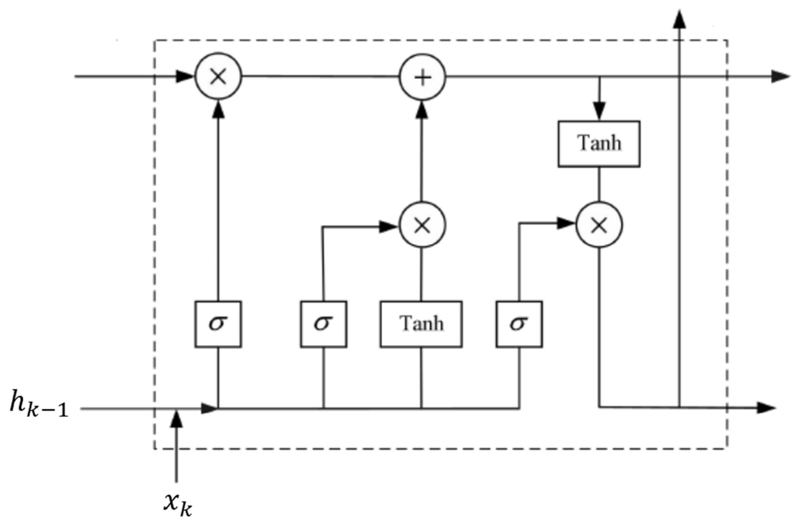
Ordinary recurrent neural networks have the disadvantage of fast decay of nodal memory, and RNNs have the disadvantage of rapidly decaying nodal memory. The LSTM model addresses both of these disadvantages [35,36]. The LSTM model contains a structure of memory units to remember past information, which is easier to train than the normal RNN [37]. The LSTM consists of three main gate structures, which are the forget gate, input gate, and output gate. The internal structure of the LSTM model is shown in Figure 2.
The forget gate mainly affects the LSTM unit at the current time by controlling historical information. The input gate is mainly used to store current information in the LSTM. The output gate determines the information that needs to be output in the current state. The LSTM is calculated by Equations (5)–(9).
f k = σ ( W f [ h k 1 , x k ] + b f )
i k = σ ( W i [ h k 1 , x k ] + b i )
C ˜ k = Tanh ( W c [ h k 1 , x k ] + b c )
o k = σ ( W o [ h k 1 , x k ] + b o )
C k = f k C k 1 + i k C ˜ k
where f k is the output of the forget gate; i k is the output of the input gate; o k is the output of the output gate; C ˜ k is the activation state of the cell; C k is the cell state at a time k; σ is the Sigmoid activation function; Tanh is the activation function; W f , W i , W c and W o are the weight matrix; h k 1 is the output value at the time k − 1; x k is the input value in the LSTM at time k; b f , b i , b c and b o are bias terms; C k 1 is the cell state at time k − 1; and is the Hadamard product of the matrix.

2.3.3. Squeeze-and-Excitation Network (SE)

The squeeze-and-excitation network is primarily used to solve the information loss situation in traditional convolutional pooling due to the same proportion of each channel in the feature map [38]. The SE obtains the weights of feature channels through autonomous learning and assigns higher weights to important channels. The SE boosts feature channels that are useful for the current task and suppresses feature channels that are of little use. The structure of SE is shown in Figure 3.
In Figure 3, X R H × W × C represents the input feature map, H and W are the length and width of the feature map and C is the number of channels. To obtain the weights of each channel of the input feature map, the SE will perform the squeeze-and-excitation operations.
The squeeze operation compresses the extracted features by performing a global average pooling in each channel and embedding the values corresponding to the global information. The squeeze operation is calculated as follows.
Z = 1 H W i = 1 H j = 1 W X c ( i , j )
where Z is the output of matrix compression, X c is the c-th input feature matrix map, i is the length ordinal number of X c , and j is the width ordinal number of X c .
The excitation operation is used to generate the weights corresponding to each feature channel by means of a fully connected layer. The first fully connected layer performs the dimensionality reduction operation, and the second fully connected layer is used to fit the complexity of the channels. Finally, the corresponding weight matrix S c is obtained using the Sigmoid activation function. The excitation operation is calculated as follows.
S c = σ ( W 2 δ ( W 1 z ) )
where σ is the Sigmoid activation function, δ is the ReLu activation function, W 1 and W 2 are the weight matrix, and z is the output of the squeeze operation.
Finally, the weight S c is added to the original channel matrix to achieve the adjustment of channel importance, which is calculated as follows.
X c ¯ = X c S c
where represents element-by-element multiplication, and X c ¯ represents the output feature map.

2.3.4. CNN-LSTM-SE Model

To deeply explore the law of the ship’s historical navigation path, this research made full use of the data most closely related to the ship’s position information to construct the ship’s trajectory prediction model. The CNN model can extract data features and capture the dependencies among features; however, it cannot take into account the time series nature of ship trajectory data and cannot capture temporal dependencies. The LSTM model is able to capture the temporal dependencies among the data. This paper combines the advantages of the CNN and LSTM models and introduces the SE module, which assigns attention weights to the extracted features, thus improving the prediction performance of the proposed model. A ship trajectory prediction model based on CNN-LSTM- SE is shown in Figure 4.
The model consists of a convolution module, an SE module, an LSTM module and a fully connected module. The convolution module is used to receive the variables that characterize the ship’s trajectory, i.e., longitude, latitude, speed and course over ground. In addition, it captures the dependencies among the variables. The SE module is used to optimize the features extracted by the CNN module to enhance the use of effective features and suppress invalid features. The LSTM module captures the temporal dependencies among sequence data. The fully connected module consists of two linear layers that integrate and differentiate the captured features and, in turn, output the predicted values.

2.4. Evaluation Index

To verify the prediction performance of the CNN-LSTM-SE model in predicting ship trajectory, two regression evaluation indexes and three distance evaluation indexes were selected to quantitatively evaluate the prediction performance of ship trajectory. The regression evaluation indexes are average root mean squared error (ARMSE) and average mean absolute percentage error (AMAPE). The three distance evaluation indexes are the average Euclidean distance (AED), the average ground distance (AGD), and the Fréchet distance (FD). The formulae are shown in Equations (13)–(17) [39,40]. In this case, the average field distance (km) is calculated according to the Haversine formula.
ARMSE = 1 2 [ 1 n i = 1 n ( l g ^ i l g i ) 2 + 1 n i = 1 n ( l t ^ i l t i ) 2 ]
AMAPE   = 1 2 n i = 1 n ( | l g ^ i l g i l g i | + | l t ^ i l t i l t i | ) × 100 %
AED = 1 n i = 1 n ( l g ^ i l g i ) 2 + ( l t ^ i l t i ) 2
A G D = 2 R n i = 1 n arcsin [ sin 2 ( Δ β i 2 ) + cos ( β i ) cos ( β ^ i ) sin 2 ( Δ α i 2 ) ]
F D = m a x ( d { ( l g ^ i , l t ^ i ) , ( l g i , l t i ) } )
where n is the predicted sample size, l g is the true value of longitude, l g ^ is the predicted value of longitude, l t is the true value of latitude, l t ^ is the predicted value of latitude, α, β, α ^ , β ^ are the radian regime quantities corresponding to the true and predicted values of latitude and longitude, respectively; α = ( l g × π ) / 180 , β and α ^ are calculated in the same way, Δ α = α ^ α , Δ β = β ^ β , R is the radius of the Earth, R = 6371   km , α ( t ) , β ( t ) are the motion position description functions, and d denotes the Euclidean distance.

3. Experiments

3.1. Experimental Setup

To verify the superiority and demonstrate the practicality of the CNN-LSTM-SE model, several experiments were conducted in this study. The experimental environment consists of hardware and software. The hardware environment included Lenovo’s Intel® Core™ i5-1135G7 with a CPU frequency of 2.40 GHz. The RAW was 16 GB, and the GPU was NVDIA GeForce GTX 750Ti. The Windows 10 operating system was used. The programming language for prediction experiments was Python 3.8; Pytorch 1.10 was also used.

3.2. Experimental Data

The AIS data can be obtained from both public-accessible databases (for free) and merchant websites [41]. The AIS raw data is complex, and the amount of information is enormous. AIS data includes mainly dynamic information (including ship location, speed, course, heading, rate of turn, destination, and estimated arrival time) as well as static information (including ship name, ship MMSI ID, message ID, ship type, ship size, and current time). The task of predicting the ship’s trajectory is mainly based on dynamic information, so only the dynamic information is used in this paper to construct the ship’s trajectory prediction model. AIS data of two cargo ships from 18 October 2022 to 23 October 2022 near the entrance of the Yangtze River in China were downloaded from the database for the experiment. Due to the high demand for cargo ship transportation in China, two cargo ships entering and leaving the Yangtze estuary were analyzed. The aim was to validate the performance of the model and to further analyze the ship control strategy. For ease of distinction, the cargo ship with a length of 264 m was labeled as ship-1, and the cargo ship with a length of 75 m was labeled as ship-2. The data size of ship-1 was 276, and the data size of ship-2 was 351.
To test the predictive effect of the model short periods, two sets of six simulation experiments were conducted. The lead time of the prediction were set to 10 s, 30 s and 1 min, respectively. The interpolated dataset was resampled for the prediction experiments [42]. In every simulation experiment, the proposed model was compared with the CNN-LSTM, CNN and LSTM models to verify the accuracy of the proposed method. In the selected data sample, the training set was 70% of the data set and the remaining 30% was the test set. After many tests on the influence of different lengths of historical navigation data on future trajectories, 1 h of historical navigation data was finally chosen as the historical data input. The parameters of the model have a great influence on the experimental results, and there is no fixed rule for parameter settings. To effectively compare the predictions, the parameters of the other models should be consistent with CNN-LSTM-SE. Through many experiments, the parameters of each model were set. Table 1 shows the parameter settings of the study. In addition, the epoch was set as 1000, the leaning rate was 0.001, the batch size was 32 and the loss function was MSE.

3.3. Results

3.3.1. Analysis of Ship-1 Trajectory Prediction Results

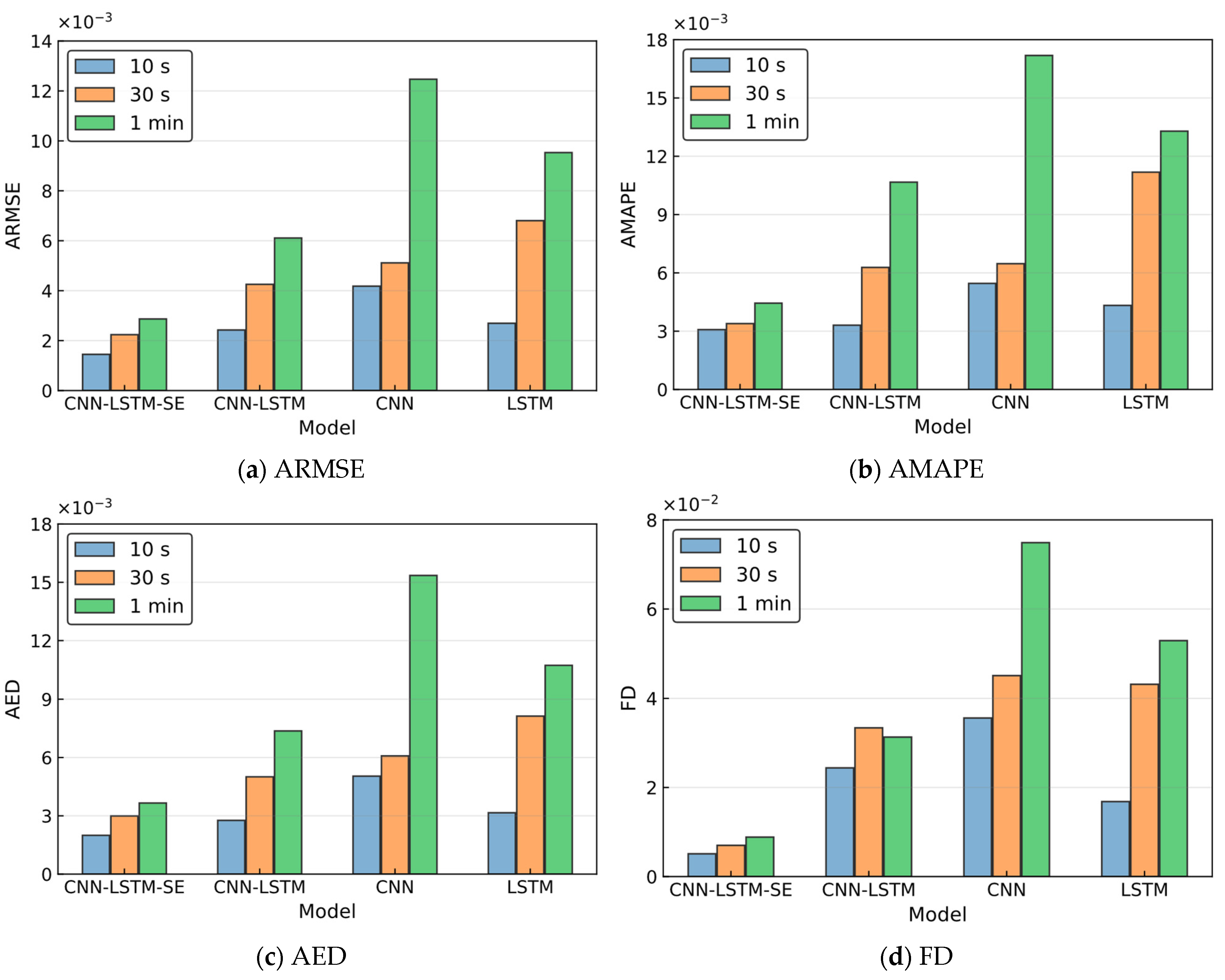
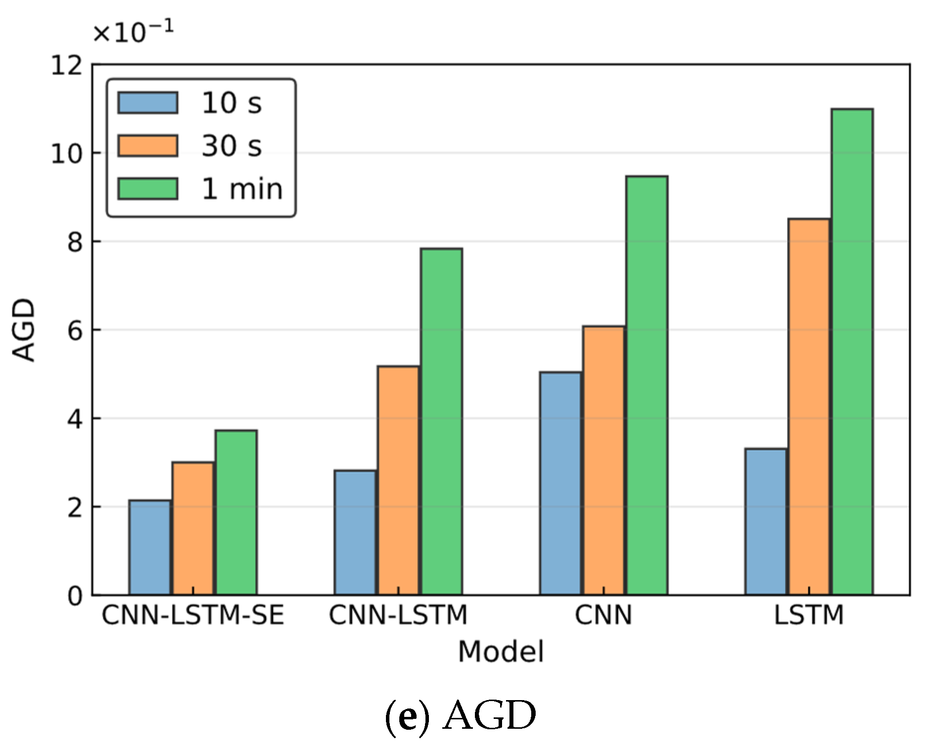
The AIS dataset from ship-1 was used for experimental analysis to test the proposed model. The evaluation index values for the various trajectory prediction models were calculated, and the results are shown in Table 2. The distribution tendency of the evaluation indexes is shown in Figure 5. At all three time intervals, the CNN-LSTM-SE model showed the best prediction effects, while the CNN model and the LSTM model presented poorer prediction effects. When the time interval was 10 s, the evaluation index values (i.e., ARMSE, AMAPE, AED, FD and AGD) of the CNN-LSTM-SE model were 0.0014, 0.0031, 0.0020, 0.0051 and 0.2141, respectively, and for the CNN-LSTM model, the evaluation index values were 0.0024, 0.0033, 0.0028, 0.0244 and 0.2816, respectively. It can be seen that the CNN-LSTM-SE model proposed in this paper achieved deep extraction of data features and improved the fitting accuracy of the model.
As the time interval increased, the prediction effect of CNN-LSTM-SE, CNN-LSTM, CNN and LSTM became increasingly inaccurate. When the time interval was 10 s, in comparison with other models, the CNN model had the worst prediction effect. For the CNN model, the evaluation index values were 0.0042, 0.0055, 0.0050, 0.0356 and 0.5037, respectively. It is easy to see that the CNN model had difficulty capturing the correlation of the trajectory data at the 10 s time interval, which seriously impacted the prediction effect. The CNN-LSTM-SE method improved the model’s ability to extract features by introducing the squeeze-and-excitation network, and the LSTM module was able to effectively capture temporal dependencies, which greatly improved its prediction effect.
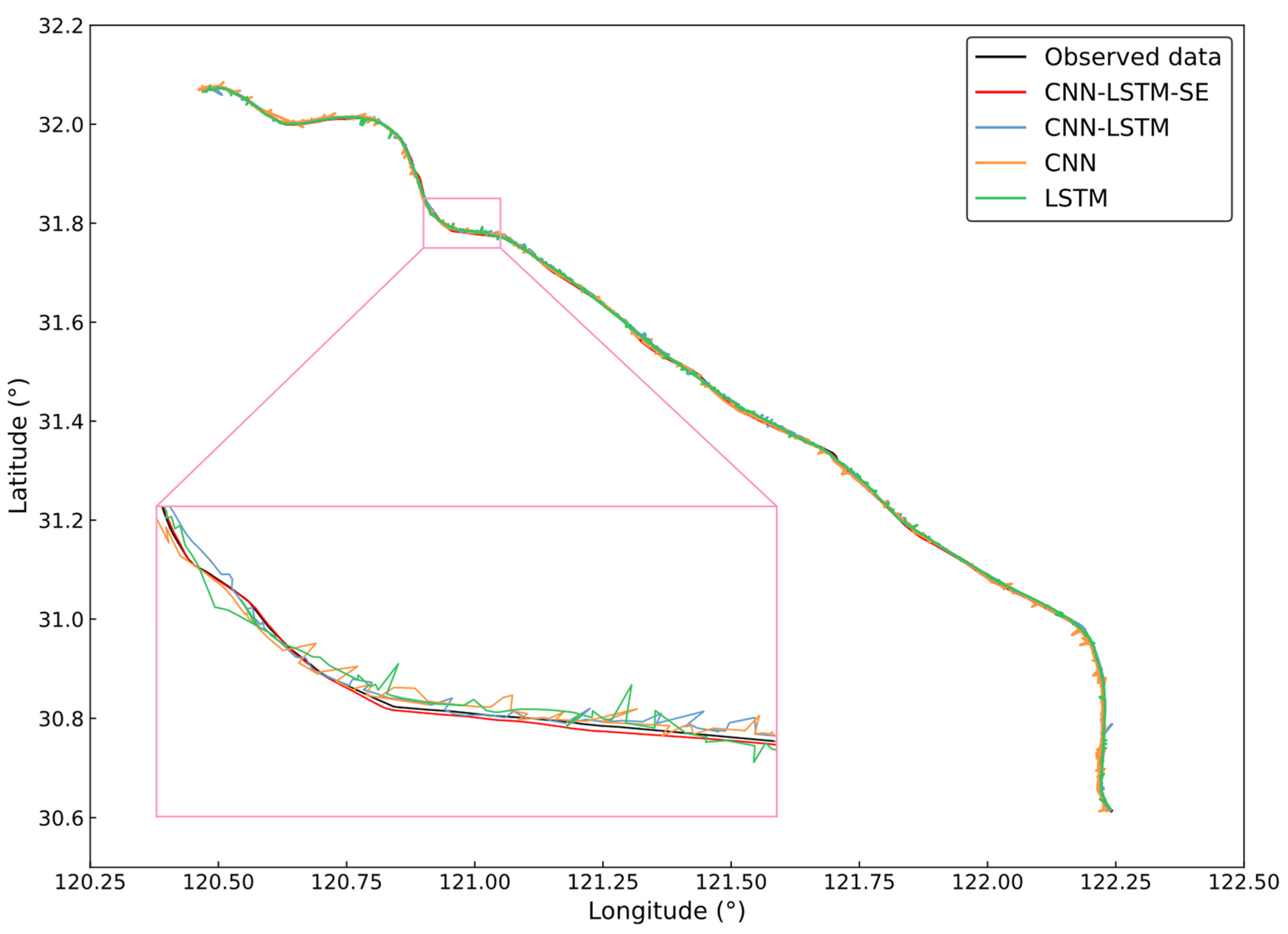
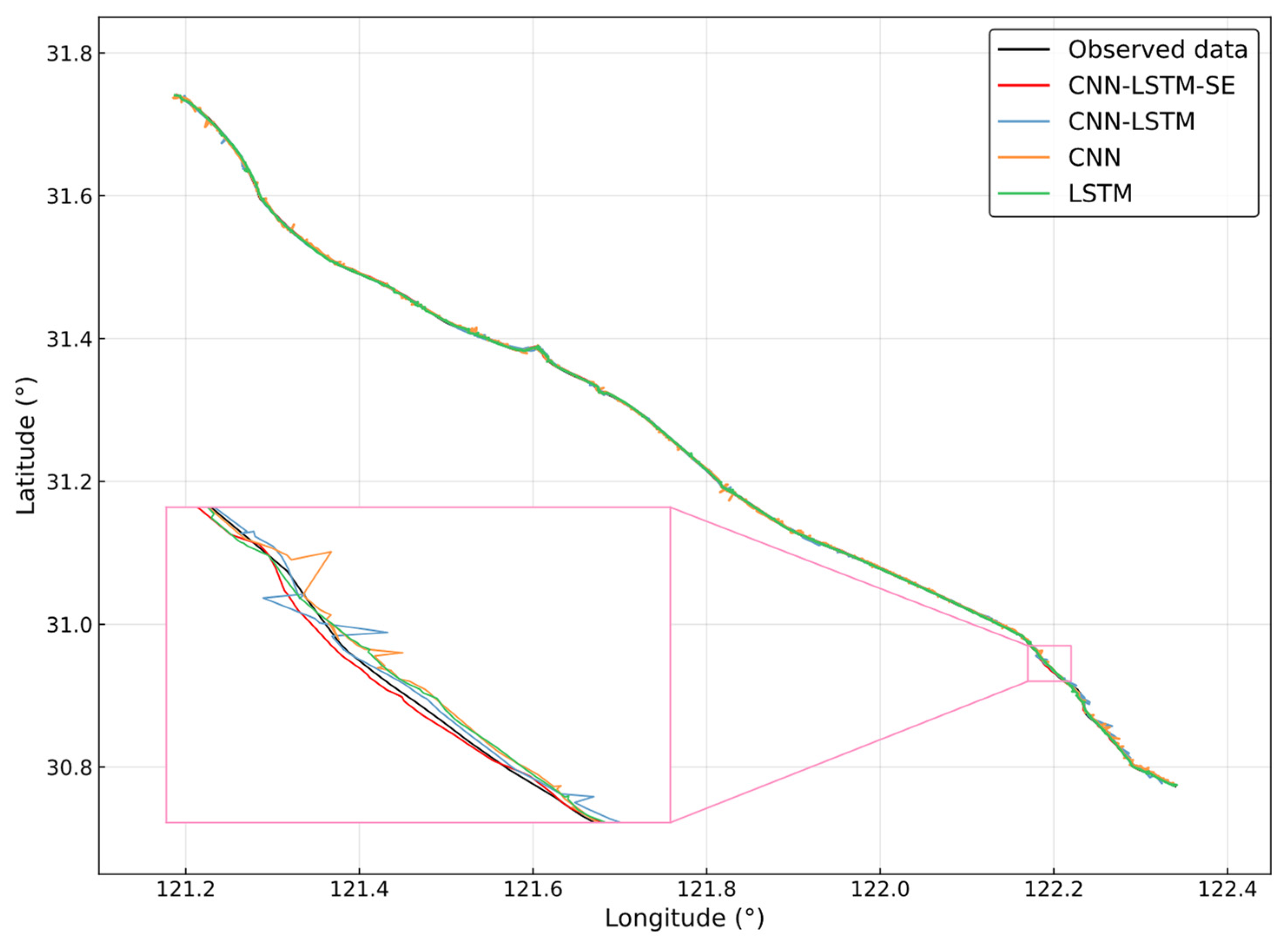
This paper shows the results of the ship-1 trajectory prediction with a time interval of 10 s. A visual representation of the trajectory prediction effect of each model is shown in Figure 6. To better compare the prediction effect of these models and better differentiate the trajectories, the partial trajectory of ship-1 is enlarged and analyzed (see the pink box in the Figure 6). As can be seen from Figure 6, the trajectory predicted by the CNN-LSTM-SE model is almost coincident with the actual trajectory of ship-1, and the other models have a poorer prediction effect, which is consistent with the evaluation index results. The comparative models predict the same general trend of the ship trajectory but still deviate from the actual trajectory, which has a large volatility. By introducing the squeeze-and-excitation network, the CNN-LSTM-SE model not only improves the ability to extract features, but also enables the whole model to be fitted with high accuracy.

3.3.2. Analysis of Ship-2 Trajectory Prediction Results

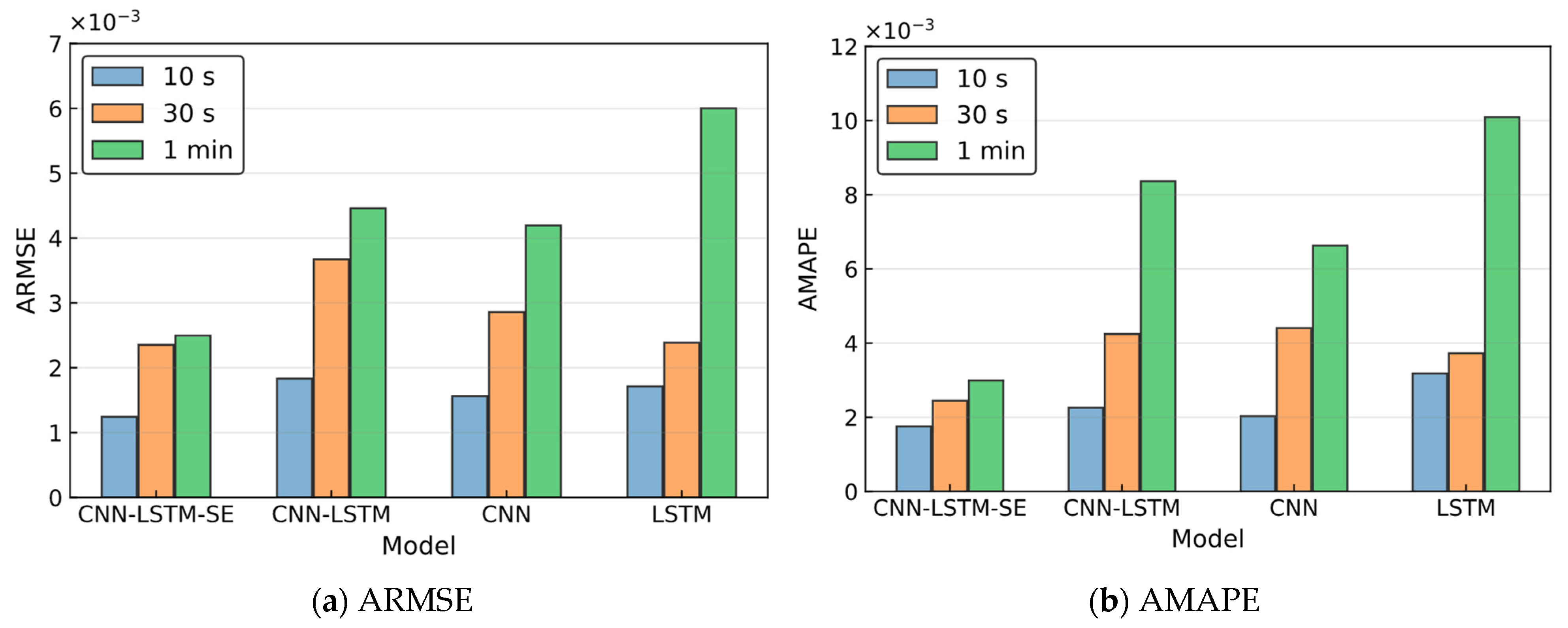
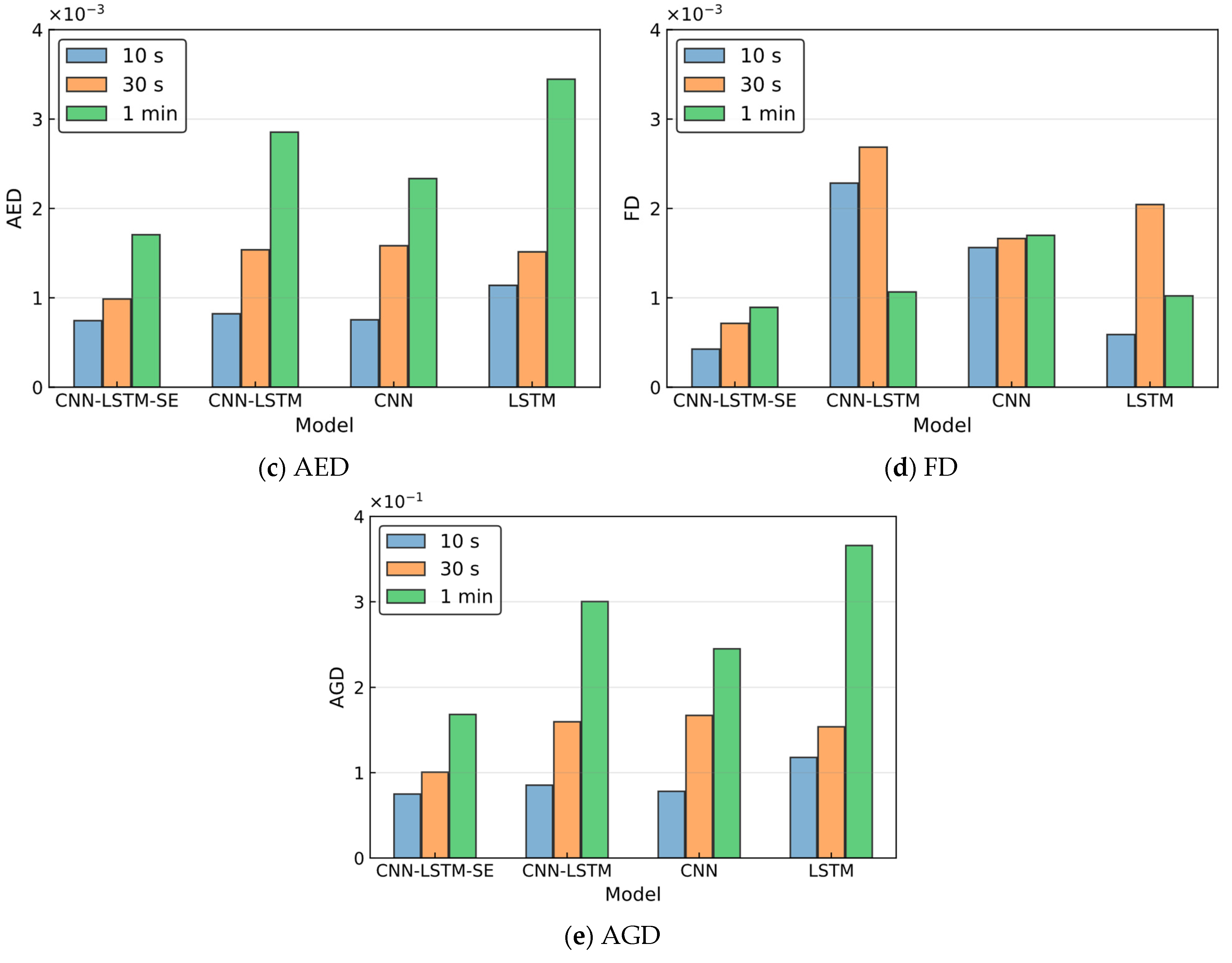
In Table 3, the ship trajectory prediction results for the ship-2 data set are given. The distribution of the evaluation index results is shown in Figure 7. In general, the CNN-LSTM-SE model is the best for ship trajectory prediction, and the comparative models are less effective. For example, at a time interval of 10 s, the evaluation index values (ARMSE, AMAPE, AED, FD and AGD) for the CNN-LSTM-SE model are 0.0012, 0.0018, 0.0007, 0.0043 and 0.0750, respectively. The CNN model does not have as good a prediction effect, with values of 0.0016, 0.002, 0.0008, 0.0156 and 0.0781, respectively. It is easy to see that the CNN-LSTM-SE model introduces the squeeze-and-excitation network based on CNN mining of correlation features of time series data, which improves prediction accuracy. In addition, the prediction effect of each model on the ship navigation trajectory gradually deteriorated as the time interval increased.
Combining Table 3 and Figure 7, compared to other models, the CNN-LSTM-SE model highlights the best ship trajectory prediction effect at different time intervals. At the time interval of 30 s, the LSTM model had a better prediction effect than the CNN model, indicating that the LSTM model can more accurately capture the time dependence of the navigation trajectory data at this time interval. The CNN-LSTM-SE model has the ability of the LSTM model to accurately capture the time dependence of serial data, improving the model’s ability to extract data features through the introduction of the squeeze-and-excitation network, which greatly improves the predictive performance of the model.
Figure 8 illustrates the effect of ship-2’s predicted trajectory at the time interval of 10 s. To better compare the prediction effect and visually distinguish the trajectories, part of the ship-2 trajectory is enlarged and compared for analysis (see the pink box in Figure 8). From Figure 8, it is easy to see that the predicted trajectory obtained from the CNN-LSTM-SE model fits the real trajectory the best and has better prediction performance, further validating the effectiveness and feasibility of CNN-LSTM-SE.

4. Conclusions

The development of international trade at sea has led to a significant increase in ship traffic, causing increased loads in navigable areas and congestion in channels, also leading to a high incidence of maritime traffic accidents. In a complex and crowded maritime environment, it is vital to ensure the safety of navigation at sea. This study proposed a CNN-LSTM-SE model to fulfill the ship trajectory prediction task. We verified the prediction performance of a proposed model at different time intervals (i.e., 10 s, 30 s and 1 min) with the help of ship AIS data samples. Moreover, we evaluated the proposed model’s accuracy compared with the other three models (i.e., CNN-LSTM model, CNN model and LSTM model). The comparison of experimental results illustrated that the proposed CNN-LSTM-SE model obtains the best prediction accuracy compared to the other models at different time intervals tested in terms of ARMSE, AMAPE, AED, AGD, and FD indicators. Moreover, the CNN-LSTM model obtained better performance than the CNN model and LSTM model for these indicators.
The prediction model proposed in this paper achieved its best prediction performance at a time interval of 10 s and its worst at an interval of 1 min. The predictive effect of the model long periods has not been verified in the experiment. Future research can focus on the long-term prediction. In future research, high-precision prediction models can be developed for long-term prediction of ship trajectories, and ship trajectories in a variety of navigational environments can be used for an example analysis.

Author Contributions

Conceptualization, X.W. and Y.X.; methodology, X.W.; investigation, X.W.; resources, Y.X.; data curation, X.W.; writing—original draft preparation, X.W.; writing—review and editing, X.W. and Y.X.; funding acquisition, Y.X. All authors have read and agreed to the published version of the manuscript.

Funding

This research was funded by the National Nature Science Foundation of China (51909155) and the Science and Technology Commission of Shanghai Municipality (22010502000, 23010501900), and was supported by the Shanghai High-level Local University Innovation Team "Maritime Safety and Security".

Institutional Review Board Statement

Not applicable.

Informed Consent Statement

Not applicable.

Data Availability Statement

The data used to support the findings of this study are available from the corresponding author upon request.

Conflicts of Interest

The authors declare no conflict of interest.

References

  1. Ma, D.; Ma, W.; Hao, S.; Jin, S.; Qu, F. Ship’s Response to Low-Sulfur Regulations: From the Perspective of Route, Speed and Refueling Strategy. Comput. Ind. Eng. 2021, 155, 107140. [Google Scholar] [CrossRef]
  2. Benz, L.; Münch, C.; Hartmann, E. Development of a Search and Rescue Framework for Maritime Freight Shipping in the Arctic. Transp. Res. A Policy Pract. 2021, 152, 54–69. [Google Scholar] [CrossRef]
  3. Zhou, Y.; Daamen, W.; Vellinga, T.; Hoogendoorn, S. Review of Maritime Traffic Models from Vessel Behavior Modeling Perspective. Transp. Res. Part C Emerg. Technol. 2019, 105, 323–345. [Google Scholar] [CrossRef]
  4. Guo, S.; Mou, J.; Chen, L.; Chen, P. An Anomaly Detection Method for AIS Trajectory Based on Kinematic Interpolation. J. Mar. Sci. Eng. 2021, 9, 609. [Google Scholar] [CrossRef]
  5. Liu, H.; Liu, Y.; Li, B.; Qi, Z. Ship Abnormal Behavior Detection Method Based on Optimized GRU Network. J. Mar. Sci. Eng. 2022, 10, 249. [Google Scholar] [CrossRef]
  6. Chen, K.; Zhu, Y.; Yan, K.; Cai, Y.; Ren, Z.; Gao, D. The Ship Track Prediction Method Based on Long Short-term Memory Network. Ship Ocean Eng. 2019, 48, 121–125. [Google Scholar] [CrossRef]
  7. Gao, M.; Shi, G.-Y. Ship-Handling Behavior Pattern Recognition Using Ais Sub-Trajectory Clustering Analysis Based on the T-Sne and Spectral Clustering Algorithms. Ocean Eng. 2020, 205, 106919. [Google Scholar] [CrossRef]
  8. Murray, B.; Perera, L.P. Ship behavior prediction via trajectory extraction-based clustering for maritime situation awareness. J. Ocean Eng. Sci. 2022, 7, 1–13. [Google Scholar] [CrossRef]
  9. Rodger, M.; Guida, R. Classification-Aided SAR and AIS Data Fusion for Space-Based Maritime Surveillance. Remote Sens. 2021, 13, 104. [Google Scholar] [CrossRef]
  10. Murray, B.; Perera, L.P. A Dual Linear Autoencoder Approach for Vessel Trajectory Prediction Using Historical Ais Data. Ocean Eng. 2020, 209, 107478. [Google Scholar] [CrossRef]
  11. Gao, D.; Zhu, Y.; Zhang, J.; He, Y.; Yan, K.; Yan, B. A Novel MP-LSTM Method for Ship Trajectory Prediction Based on Ais Data. Ocean Eng. 2021, 228, 108956. [Google Scholar] [CrossRef]
  12. Feng, H.; Cao, G.; Xu, H.; Ge, S. IS-STGCNN: An Improved Social spatial-temporal graph convolutional neural network for ship trajectory prediction. Ocean Eng. 2022, 266, 112960. [Google Scholar] [CrossRef]
  13. Liu, R.W.; Liang, M.; Nie, J.; Lim, W.Y.B.; Zhang, Y.; Guizani, M. Deep Learning-Powered Vessel Trajectory Prediction for Improving Smart Traffic Services in Maritime Internet of Things. IEEE Trans. Netw. Sci. Eng. 2022, 9, 3080–3094. [Google Scholar] [CrossRef]
  14. Chen, X.; Wei, C.; Zhou, G.; Wu, H.; Wang, Z.; Biancardo, S.A. Automatic Identification System (AIS) Data Supported Ship Trajectory Prediction and Analysis via a Deep Learning Model. J. Mar. Sci. Eng. 2022, 10, 1314. [Google Scholar] [CrossRef]
  15. Qian, L.; Zheng, Y.; Li, L.; Ma, Y.; Zhou, C.; Zhang, D. A New Method of Inland Water Ship Trajectory Prediction Based on Long Short-Term Memory Network Optimized by Genetic Algorithm. Appl. Sci. 2022, 12, 4073. [Google Scholar] [CrossRef]
  16. Liu, J.; Shi, G.; Zhu, K. Vessel Trajectory Prediction Model Based on AIS Sensor Data and Adaptive Chaos Differential Evolution Support Vector Regression (ACDE-SVR). Appl. Sci. 2019, 9, 2983. [Google Scholar] [CrossRef] [Green Version]
  17. Zhang, L.; Zhang, J.; Niu, J.; Wu, Q.M.J.; Li, G. Track Prediction for HF Radar Vessels Submerged in Strong Clutter Based on MSCNN Fusion with GRU-AM and AR Model. Remote Sens. 2021, 13, 2164. [Google Scholar] [CrossRef]
  18. Volkova, T.A.; Balykina, Y.E.; Bespalov, A. Predicting Ship Trajectory Based on Neural Networks Using AIS Data. J. Mar. Sci. Eng. 2021, 9, 254. [Google Scholar] [CrossRef]
  19. Park, J.; Jeong, J.; Park, Y. Ship Trajectory Prediction Based on Bi-LSTM Using Spectral-Clustered AIS Data. J. Mar. Sci. Eng. 2021, 9, 1037. [Google Scholar] [CrossRef]
  20. Suo, Y.; Chen, W.; Claramunt, C.; Yang, S. A Ship Trajectory Prediction Framework Based on a Recurrent Neural Network. Sensors 2020, 20, 5133. [Google Scholar] [CrossRef]
  21. Bao, K.; Bi, J.; Gao, M.; Sun, Y.; Zhang, X.; Zhang, W. An Improved Ship Trajectory Prediction Based on AIS Data Using MHA-BiGRU. J. Mar. Sci. Eng. 2022, 10, 804. [Google Scholar] [CrossRef]
  22. Sørensen, K.A.; Heiselberg, P.; Heiselberg, H. Probabilistic Maritime Trajectory Prediction in Complex Scenarios Using Deep Learning. Sensors 2022, 22, 2058. [Google Scholar] [CrossRef] [PubMed]
  23. Zhao, J.; Lu, J.; Chen, X.; Yan, Z.; Yan, Y.; Sun, Y. High-fidelity data supported ship trajectory prediction via an ensemble machine learning framework. Phys. A 2022, 586, 126470. [Google Scholar] [CrossRef]
  24. Gao, D.; Zhu, Y.; Soares, C.G. Uncertainty modelling and dynamic risk assessment for long-sequence AIS trajectory based on multivariate Gaussian Process. Reliab. Eng. Syst. Safe 2023, 230, 108963. [Google Scholar] [CrossRef]
  25. Zheng, Y.; Li, L.; Qian, L.; Cheng, B.; Hou, W.; Zhuang, Y. Sine-SSA-BP Ship Trajectory Prediction Based on Chaotic Mapping Improved Sparrow Search Algorithm. Sensors 2023, 23, 704. [Google Scholar] [CrossRef]
  26. Wang, Y.; Xu, S.; Feng, D. A New Method for Short-Term Traffic Flow Prediction Based on Multi-Segments Features. In Proceedings of the 2020 12th International Conference on Machine Learning and Computing, Shenzhen, China, 15–17 February 2020; ACM: New York, NY, USA, 2020; pp. 34–38. [Google Scholar] [CrossRef]
  27. Zhao, T.; Wu, X. Pyramid Feature Attention Network for Saliency Detection. In Proceedings of the 2019 IEEE/CVF Conference on Computer Vision and Pattern Recognition (CVPR), Long Beach, CA, USA, 15–20 June 2019; IEEE: Piscataway, NJ, USA, 2019; pp. 3080–3089. [Google Scholar] [CrossRef] [Green Version]
  28. Wang, K.; Ma, C.; Qiao, Y.; Lu, X.; Hao, W.; Dong, S. A Hybrid Deep Learning Model with 1dcnn-Lstm-Attention Networks for Short-Term Traffic Flow Prediction. Phys. A Stat. Mech. Appl. 2021, 583, 126293. [Google Scholar] [CrossRef]
  29. Hu, Y.K.; Xia, W.; Hu, X.X.; Sun, H.Q.; Wang, Y.H. Prediction of Ship Track Based on Recurrent Neural Network. Sys. Eng. Elect. Technol. 2020, 42, 871–877. [Google Scholar] [CrossRef]
  30. Capobianco, S.; Millefiori, L.M.; Forti, N.; Braca, P.; Willett, P. Deep Learning Methods for Vessel Trajectory Prediction Based on Recurrent Neural Networks. IEEE Trans. Aero. Elec. Sys. 2021, 57, 4329–4346. [Google Scholar] [CrossRef]
  31. Tengesdal, T.; Johansen, T.A.; Brekke, E.F. Ship Collision Avoidance Utilizing the Cross-Entropy Method for Collision Risk Assessment. IEEE Trans. Intell. Transp. Syst. 2022, 23, 11148–11161. [Google Scholar] [CrossRef]
  32. Liu, Z.; Zhuang, Y.; Jia, P.; Wu, C. A Novel Underwater Image Enhancement and Improved Underwater Biological Detection Pipeline. arXiv 2022. [Google Scholar] [CrossRef]
  33. Wu, S.; Chen, X.; Shi, C.; Shi, C.; Fu, J.; Wang, S. Ship detention prediction via feature selection scheme and support vector machine (SVM). Marit. Policy Manag. 2022, 49, 140–153. [Google Scholar] [CrossRef]
  34. Zhao, J.; Yan, Z.; Chen, X.; Han, B.; Wu, S.; Ke, R. k-GCN-LSTM: A k-hop Graph Convolutional Network and Long–Short-Term Memory for ship speed prediction. Phys. A 2022, 606, 128107. [Google Scholar] [CrossRef]
  35. Cornia, M.; Baraldi, L.; Serra, G.; Cucchiara, R. Predicting Human Eye Fixations via an LSTM-Based Saliency Attentive Model. IEEE Trans. Image Process. 2018, 27, 5142–5154. [Google Scholar] [CrossRef] [Green Version]
  36. Li, Z.-Y.; Yu, C.-H.; Lin, Y.-T.; Su, H.-L.; Kan, K.-W.; Liu, F.-C.; Chen, C.-T.; Lin, Y.-T.; Hsu, H.-F.; Lin, Y.-H. The Potential Application of Spring Sargassum glaucescens Extracts in the Moisture-Retention of Keratinocytes and Dermal Fibroblast Regeneration after UVA-Irradiation. Cosmetics 2019, 6, 17. [Google Scholar] [CrossRef] [Green Version]
  37. Ran, X.; Shan, Z.; Fang, Y.; Lin, C. An LSTM-Based Method with Attention Mechanism for Travel Time Prediction. Sensors 2019, 19, 861. [Google Scholar] [CrossRef] [PubMed] [Green Version]
  38. Hu, J.; Shen, L.; Sun, G. Squeeze-and-Excitation Networks. In Proceedings of the IEEE Conference on Computer Vision and Pattern Recognition, Salt Lake City, UT, USA, 18–23 June 2018; IEEE: Piscataway, NJ, USA, 2018; pp. 7132–7141. [Google Scholar]
  39. Peng, Y.; Xiang, W. Short-Term Traffic Volume Prediction Using GA-BP Based on Wavelet Denoising and Phase Space Reconstruction. Phys. A 2020, 549, 123913. [Google Scholar] [CrossRef]
  40. Wang, W.; Zhang, H.; Li, T.; Guo, J.; Huang, W.; Wei, Y.; Cao, J. An Interpretable Model for Short Term Traffic Flow Prediction. Math. Comput. Simul. 2020, 171, 264–278. [Google Scholar] [CrossRef]
  41. Mazzarella, F.; Vespe, M.; Alessandrini, A.; Tarchi, D.; Aulicino, G.; Vollero, A. A novel anomaly detection approach to identify intentional AIS on-off switching. Expert Syst. Appl. 2017, 78, 110–123. [Google Scholar] [CrossRef]
  42. Wang, S.; He, Z. A Prediction Model of Vessel Trajectory Based on Generative Adversarial Network. J. Navig. 2021, 74, 1161–1171. [Google Scholar] [CrossRef]
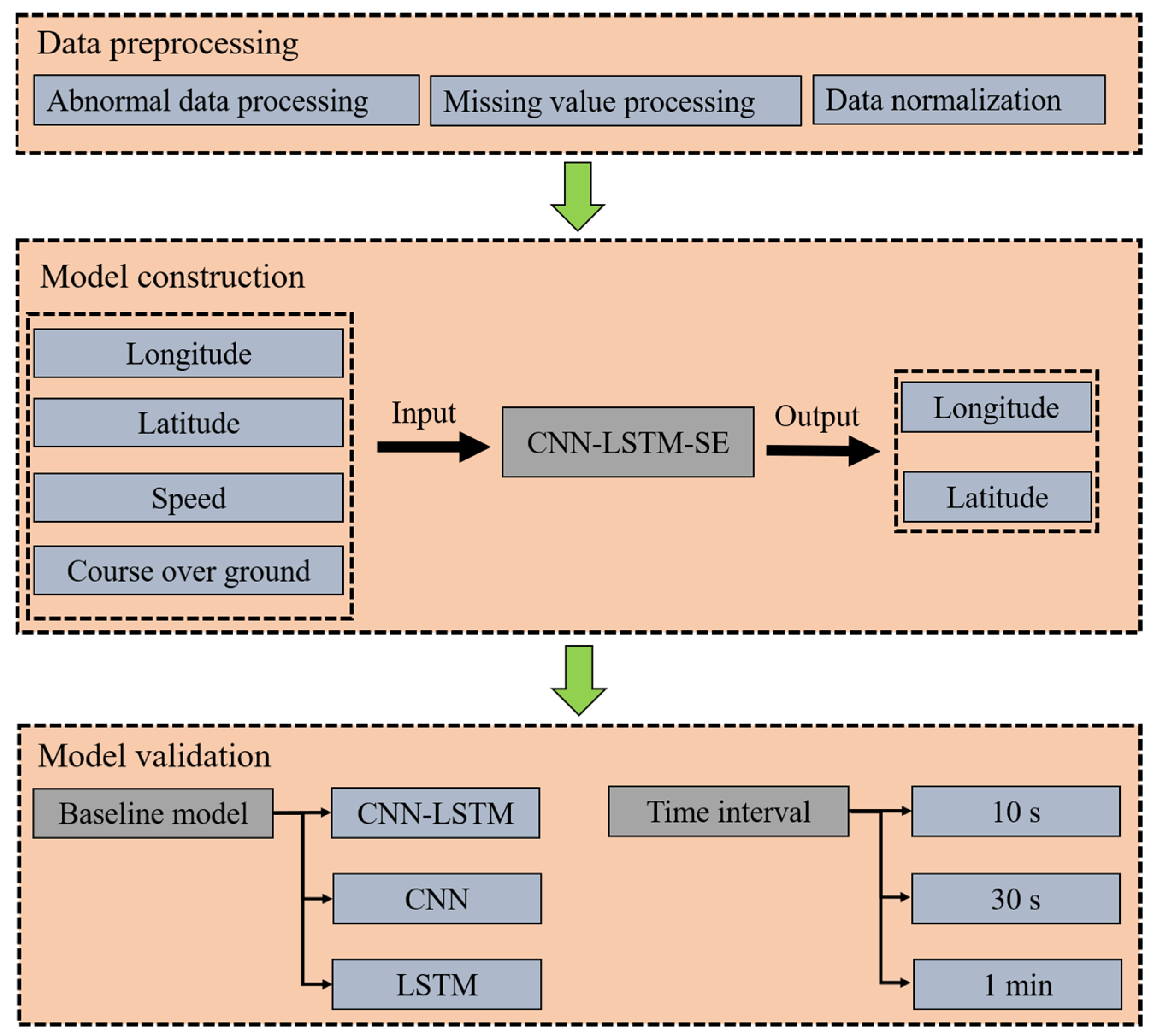
Figure 1. The research framework of the ship trajectory prediction method.
Information 14 00212 g001
Figure 2. The cell structure of the LSTM.
Information 14 00212 g002
Figure 3. The squeeze-and-excitation network structure.
Information 14 00212 g003
Figure 4. The overall structure of the prediction model.
Information 14 00212 g004
Figure 5. Distribution of evaluation indexes of ship-1.
Information 14 00212 g005aInformation 14 00212 g005b
Figure 6. Performance of prediction models for ship-1 with a time interval of 10 s.
Information 14 00212 g006
Figure 7. Distribution of evaluation indexes of ship-2.
Information 14 00212 g007aInformation 14 00212 g007b
Figure 8. Performance of prediction models for ship-2 with a time interval of 10 s.
Information 14 00212 g008
Table 1. Model parameter settings.
ModelTime IntervalParameter NameOptimal Parameters
CNN-LSTM-SE10 sKernel size2
Stride2
LSTM node300
Linear layer node100
Output layer node2
30 sKernel size2
Stride1
LSTM node300
Linear layer node100
Output layer node2
1 minKernel size2
Stride1
LSTM node150
Linear layer node50
Output layer node2
Table 2. Trajectory prediction results of ship-1.
Time IntervalModelARMSEAMAPEAEDFDAGD
10 sCNN-LSTM-SE0.00140.00310.00200.00510.2141
CNN-LSTM0.00240.00330.00280.02440.2816
CNN0.00420.00550.00500.03560.5037
LSTM0.00270.00430.00320.01680.3308
30 sCNN-LSTM-SE0.00220.00340.00300.00700.3001
CNN-LSTM0.00430.00630.00500.03340.5171
CNN0.00510.00650.00610.04510.6077
LSTM0.00680.01120.00810.04320.8504
1 minCNN-LSTM-SE0.00290.00440.00370.00890.3721
CNN-LSTM0.00610.01070.00740.03130.7831
CNN0.01250.01720.01540.07490.9467
LSTM0.00950.01330.01070.05291.0987
Table 3. Trajectory prediction results of ship-2.
Time IntervalModelARMSEAMAPEAEDFDAGD
10 sCNN-LSTM-SE0.00120.00180.00070.00430.0750
CNN-LSTM0.00180.00230.00080.02280.0854
CNN0.00160.00200.00080.01560.0781
LSTM0.00170.00320.00110.00590.1179
30 sCNN-LSTM-SE0.00240.00240.00100.00710.1006
CNN-LSTM0.00370.00420.00150.02690.1597
CNN0.00290.00440.00160.01660.1671
LSTM0.00240.00370.00150.02040.1538
1 minCNN-LSTM-SE0.00250.00300.00170.00890.1682
CNN-LSTM0.00450.00840.00290.01070.3002
CNN0.00420.00660.00230.01700.2448
LSTM0.00600.01010.00340.01020.3659
Disclaimer/Publisher’s Note: The statements, opinions and data contained in all publications are solely those of the individual author(s) and contributor(s) and not of MDPI and/or the editor(s). MDPI and/or the editor(s) disclaim responsibility for any injury to people or property resulting from any ideas, methods, instructions or products referred to in the content.