Intrinsically Interpretable Gaussian Mixture Model

Abstract

Understanding the reasoning behind a predictive model’s decision is an important and longstanding problem driven by ethical and legal considerations. Most recent research has focused on the interpretability of supervised models, whereas unsupervised learning has received less attention. However, the majority of the focus was on interpreting the whole model in a manner that undermined accuracy or model assumptions, while local interpretation received much less attention. Therefore, we propose an intrinsic interpretation for the Gaussian mixture model that provides both global insight and local interpretations. We employed the Bhattacharyya coefficient to measure the overlap and divergence across clusters to provide a global interpretation in terms of the differences and similarities between the clusters. By analyzing the GMM exponent with the Garthwaite–Kock corr-max transformation, the local interpretation is provided in terms of the relative contribution of each feature to the overall distance. Experimental results obtained on three datasets show that the proposed interpretation method outperforms the post hoc model-agnostic LIME in determining the feature contribution to the cluster assignment.

1. Introduction

Predictive modeling is ubiquitous and has been adopted in high-stakes domains as a result of its ability to make precise and reliable decisions. The General Data Protection Regulation (GDPR) in the European Union mandates that model decisions in crucial fields including medical diagnosis, credit scoring, law and justice must be understood and interpreted prior to their implementation. The notion of interpreting a model’s prediction dates back to the late 1980s [1]. Since then, there have been several efforts to improve interpretability, the majority of which have focused on supervised learning methods, such as support vector machines [2], random forests [3], and deep learning [4]. Supervised learning has the advantage of not only knowing the number of classes but also the distribution of each population. It also has access to both the learning sample and objective function to minimize an error.

Clustering, which is unsupervised learning, divides and clusters data into groups by maximizing the similarity within a group and the differences among groups. It is also useful to extract unknown patterns from data. Due to its exploratory nature, providing only cluster results is not adequate. The cluster assignments are determined using all the features of the data, which makes the inclusion of a particular point in a cluster difficult to explain. It also limits the user’s ability to discern the commonalities between points within a cluster or understand why points end up in different clusters, especially in cases of high dimensions or uncertainty.

Due to its subjective nature and lack of a consistent definition and measure, assessing interpretability is a difficult endeavor. Additionally, interpretability is extremely context-dependent (domain, target audience, data type, etc.) [5,6]. The input data type is another factor to consider when selecting an output type. For instance, a tree is an effective method for describing tabular data, but it is inadequate when attempting to explain images.

Many works have attempted to bridge this gap and provide interpretable clustering models. Nonetheless, local interpretation has received less attention and has mostly adopted model-agnostic approaches. The reliance on model-agnostic and locally approximative models fails to represent the underlying model behavior, particularly in cases of overlap or uncertainty. In addition, when offering a local interpretation that considers only a small portion of the model, the interpretation cannot represent the model logic, and thus, may be deceptive.

In this paper, we discuss developing an interpretable Gaussian mixture model (GMM) without sacrificing accuracy by considering both global and local interpretations. The interpretation of the cluster is supplied with as much specificity and distinction as feasible. The local interpretation uses the GMM exponent to identify the features that led to the assignment of a given point.

This paper first provides some background knowledge on the GMM along with the interpretability fundamentals. Second, it reviews and discusses studies on unsupervised interpretability. The proposed method is then presented, along with the results and their discussion.

2. Background

In this section, GMM and the basics of interpretability are briefly presented.

2.1. GMM

A GMM consists of several Gaussian distributions called components. Each component is added to other components to form the probability density function (PDF) of the GMM. Formally, for a random vector x the PDF of the GMM $p\left(x\right)$ is defined as follows [7]:

$$\begin{array}{c}\hfill p\left(x\right)={\Sigma }_{k=1}^K{P}_k\mathcal{N}\left(x\right|{\mu }_k,{\Sigma }_k),\end{array}$$

(1)

where $P_k$ represents the weight (mixing proportions) such that $P_k>0$, and ${\Sigma }_{k=1}^K{P}_k=1$; ${\mu }_k$ and ${\Sigma }_k$ represent the mean vector and covariance matrix of the k component, respectively; K is the number of components.

The PDF of the GMM component is [7]:

$$\begin{array}{c}\hfill \mathcal{N}\left(x\right|\mu ,\Sigma )=\frac{1}{{\left(2\pi \right)}^{D/2}{|\Sigma |}^{(1/2)}}exp\{-\frac{1}{2}{(x-\mu )}^T{\Sigma }^{-1}(x-\mu )\}\end{array}$$

(2)

Because the components might overlap, the result of GMM is not a hard assignment of a point to one cluster; rather, a point can belong to multiple clusters with a certain probability for each cluster.

2.2. Interpreteability

Interpretability aims to provide understandable model predictions to the user. Regardless of its different definitions and considerations, interpretability approaches have three main dimensions: scope, stage, and specificity (Figure 1).

Figure 1. Interpretation dimensions.

In the scope dimension approaches can be classified into two main categories: local and global. Local interpretation is provided per prediction to explain the model decision for an individual outcome, while global interpretation provides interpretation for the entire model’s behavior [8]. As the output, the local interpretation can be either feature-based, where it is provided in terms of feature contribution, e.g., feature weights [9], or saliency maps [10,11]. The other form is instance-based, which can be a similar case (prototype) [12], counterfactual [13], or the most influential example which is done by tracing back to training data [14]. Global interpretation usually takes the form of a proxy model (converting the model into a simpler one) [15] or by augmenting the interpretation within the model building process to make it intrinsic. However, because it is difficult to provide an accurate global interpretation, approaches usually rely on some proxies that compromise the model’s accuracy.

The second dimension is the stage when the interpretation takes place. The interpretation process can take place at two different stages, post hoc, where the process of providing interpretation occurs after building a model, and ante hoc (intrinsic), which occurs during the model building process.

The last dimension is specificity. Approaches can be either model-specific or model-agnostic. Model-specific approaches are restricted to one black-box model or one class of models (e.g., neural networks, CNN, or support vector machines). Model agnostic is untied to any particular type of black-box model and can be applied to any machine learning model. Agnostic models use reverse engineering approaches to reveal the underlying black-box model logic. During this process, a black box is queried with test data to produce output records, and the data are then used to approximate the original model and construct an interpretation for it.

These dimensions may overlap as one model can be post hoc and either local or global. Some examples include LIME [9], which is local, post hoc, and model agnostic, and GoldenEye [16], which is global, post hoc, and model agnostic. However, no overlap can be found between intrinsic and agnostic models.

3. Related Work

Most of the literature on interpretability covers supervised learning and particularly neural networks. Little research has been conducted on the interpretation of unsupervised learning, namely clustering.

Interpretable clustering models refer to clustering models that provide explanations as to what characterizes a cluster and how a cluster is distinguished from others.

Decision rules are among the most interpretable and understandable techniques widely used to either explain models or build transparent models.

Pelleg and Moore [17] fit data in a mixture model where each component is contained in an M-dimensional hyperrectangle, and each component has a pair of M-length vectors that define the upper $R^h$ and lower $R^l$ boundaries for every dimension (attributes). They allow overlap among hyperrectangles to allow soft-membership. In the early stages of EM, they allow rectangles to have soft tails. In the Gaussian mixture, the distance is calculated from the point to the cluster mean. In their model, the distance is measured to the closest point included in the rectangle; in other words, the distance is computed by how far away a point x is from the boundary of rectangle R, so the mean point is stretched into an interval.

The resulting clusters can then be converted into rule-based boundaries, which only consider continuous attributes.

The discriminative rectangle mixture (DReaM) [18] model utilizes the same idea. It learns a rectangular decision rule for each cluster. Domain experts are utilized to gain background knowledge and consider rules of thumb, such as clinical guidelines, in a semi-supervised manner to separate samples into groups. This makes GMM more interpretable. However, rectangular shapes may not necessarily fit the data of the clusters, so they may sacrifice accuracy in favor of interpretability. Furthermore, the resulting rules become remarkably long in high-dimensional settings. Fitting data using a rectangle approach assumes the local independence of features. This can be interpreted as assuming diagonal covariance in GMM that then takes the covariance along the diagonal of the sides of the hyperrectangle. Additionally, the transition from soft clustering to hard clustering and from elliptical modeling to rectangular modeling is a design choice that is not fully justified mathematically or grounded in probability.

In [19], the cluster interpretation is generated by optimizing a multi-objective function. In addition to centroid-based clustering objectives, the interpretability level, which measures the fraction of agreement among a cluster’s node concerning a feature’s value, is included as a tunable parameter. The authors assume that the interpretability level and feature of interest will be provided by the user. The explanation is generated as logical combinations of the feature values for the feature of interest associated with the nodes in each cluster using frequent pattern mining. The interpretation is a logical or over combinations of the feature values of the feature of interest associated with the nodes in each cluster. To quantify the interpretability, they compute an interpretability score per cluster concerning a feature value, which is given by the maximum fraction of nodes that share the feature’s value. However, in some cases, the algorithm might not converge to a local maximum to achieve the given interpretability level.

The Search for Explanations for Clusters of Process Instances (SECPI) algorithm [20], is a post hoc explanation method that applies SVMs on cluster results. SECPI takes an instance to be explained as input after converting it to a sequence of binary attributes and returns the label along with the score (probability). Adopting a winner-takes-all model (per cluster—k SVM models), the model with the highest probability determines the label along with the score. The interpretation output is a set of rules that are formalized as a set of sets of attribute indices. The explanation is interpreted as all attributes that need to be inverted, so the instance would leave its current cluster.

One strategy to improve interpretability is to describe the clusters using an example. Humans learn by example, and exemplar-based reasoning is one of the most effective strategies for tactical decision-making. In this strategy, the most representative example of the cluster, termed a prototype, is used as an interpretation.

Case-based reasoning, investigated in [12], provides an interpretable framework called the Bayesian case model (BCM) that performs joint inference on cluster labels, prototypes, and features. The BCM is composed of two parts: the first is the standard discrete mixture model to learn the structure of instances. The second part is for learning the explanation (example) by applying uniform distribution over all the data points to find the most representative instance per group (cluster). However, the authors assume the number of clusters, all the parameters, and the type of probability distributions are correct for each type of data. In addition, the data are composed of discrete values only. Moreover, being dependent on examples, interpretation is an over-generalization and a mistake that is only rectified if the distribution of the data points is clean, which is rare [21].

Carrizosa et al. [22] proposed a post hoc distance-based prototype interpretation given the dissimilarity between instances. The prototype was found over the clustering results by optimizing a bi-objective function that maximizes true positive and minimizes false positives using two methods. The first method, covering, utilizes a user-provided dissimilarity threshold for the closeness between data instances, where the distance between the prototype and an individual must be less than the threshold. In the second method, set-partitioning, an individual is assigned to the closest prototype. The authors just focused on the case where there is only one prototype per cluster with a hard clustering condition.

Decision trees are a human-understandable format; thus, many approaches consider providing the interpretation as a tree. ExKMC [23] separates each cluster from the others using a threshold cut based on a single feature to form a binary threshold three with k-leaves representing k-cluster labels, and each internal node contains a threshold value that partitions the data to form a cluster ruled by the condition from the root-to-leaf path. Essentially, they find k-centers and assign each data point to its closest center forming labels. Then, they build a binary tree to fit the clustering label, using dynamic programming to find optimal split. They just focus on k-leaves trees for each cluster to maintain only a small number of conditions. They also provide theoretical results on explainable k-means and k-medians clustering.

A two-phase interpretable model is proposed by IBM’s group [24], and the authors first applied their Locally Supervised Metric Learner (LSML) of patient similarity analytics to estimate the outcome-adjusted behavioral distances between users. Then, based on the adjusted behavioral distances, hierarchical clustering is employed to generate sub-cohorts and learn the key features (which contain behavioral signals about implicit user preferences and barriers) that drive the differential outcomes. Additionally, they provide prototypical examples that represent the 10 closest instances to the centroid.

Kim et al. [25] proposed the Mind the Gap Model (MGM), an interpretable clustering model that simultaneously decomposes observations into k clusters while returning a comprehensive list of distinguishable dimensions that allows for differentiating among clusters. MGM has two parts: interpretable feature extraction and selection. In the former, the features are grouped by a logical formula considering only and/oroperators for the sake of dimensionality reduction. Each dimension can be a member of one group (logical formula) to avoid searching all combinations of d, which is an NP-complete satisfiability problem [25]. In feature selection, the model selects the group that creates a large separation -gap- in the parameter’s value. This model is focused on binary value data.

As shown in Table 1, most of the existing works focus on categorical data [12,19,20,22,23,24]. Continuous data are considered in two works. Both works address the interpretation of GMM with rules as an interpretation output [17,18]. This is due to the difficulty of determining and handling the thresholds and intervals in continuous data. None of the existing works overcome uncertainty in the context of interpretation. They either adopt hard clustering or well-separated data.

Table 1. Related Work Summary. The column Config. contains any configuration or supplementary information that the model requires, where P-h refers to post hoc.

Ref.	Approach	Config.	Output	P-h
Continues data
[17]	Fit data in M-dimensional hyper-rectangle	# of clusters	Rule	No
[18]	Discriminative model learn rectangular decision rules	Domain expert for decision boundaries, # of clusters	Rule	No
Discrete data
[12]	Use discrete mixture model. Then apply uniform distribution over all data to find the representative instance per cluster	# of clusters	Prototype	No
[19]	Simultaneously optimize distance and interpretability	# of clusters, interpretability level, feature of interest	Rule	No
[23]	Use k-means to extract class label of cluster assignments, then return tree with k-leaves.	# of clusters	Tree	No
[24]	Supervised Learner for similarity then hierarchical clustering for key feature defining the different outcomes	Label provided by physician	Features, Prototype	Yes
[20]	After clustering data use a k SVM models (on cluster results)	attributes template, search depth, early stop parameter	Rule	Yes
[22]	Find prototype that maximize true positive and minimize false positive	dissimilarity between individuals	Prototype	Yes
Binary data
[25]	Finds set of distinguishable dimensions per cluster utilizing searching over logical formula	# of clusters	Features	No

Another shortcoming is the lack of effective evaluation in the majority of the literature, which either focuses on cluster objectives or provides only a theoretical analysis.

To the best of our knowledge, the literature on clustering only provides a global interpretation, which results in useful insight into inner workings. However, it is still necessary to follow the decision-making process of a new observation, i.e., to provide a local interpretation of a new instance.

The local interpretation in clusters can be provided by relying on a post hoc model agnostic such as the Local Interpretable Model-Agnostic Explanations (LIME) [9], and SHapley Additive exPlanations (SHAP) [26]. However, it has been demonstrated that post hoc techniques that rely on input perturbations, such as LIME and SHAP, are not reliable [27].

4. Contribution: Intrinsic GMM Interpretations

In the context of clustering, interpretability refers to a cluster’s characteristics and how it is distinguished from other clusters. In our work, we explain a cluster’s similarities and differences by utilizing the overlap. If two clusters overlap a feature, it implies that they have similarities in that feature; thus, we exclude it from the distinguishing list between those two clusters.

To determine key features globally per cluster, we eliminate highly overlapped features. Locally, the key features are determined through an exponent analysis.

4.1. Global Interpretation

Global interpretation provides useful insight into the inner workings of the latent space. It highlights the relationship and differences among classes. Our approach focuses on finding differences between clusters and commonalities by utilizing the overlap coefficient. Determining the overlap helps to provide sub-feature values that are important for characterizing a cluster.

The cluster overlapping phenomenon is not well characterized mathematically, especially in multivariate cases [28]. It affects a human’s ability to perceive the cluster assignment and has a strong impact on the prediction certainty which affects the interpretability of the resulting clusters.

Many measures were designed to capture the overlap/similarity between two probability distributions. Following Krzanowski [29], those measures can be broadly classified into two categories. The first category is measures based on ideas from information theory such as Kullback & Leibler’s [30] and Sibson’s [31] measures. The second category represents measures related to the Bhattacharyya measure of affinity, such as Bhattacharyya [32] and Matusita [33].

The Bhattacharyya coefficient $BC$ reflects the amount of overlap between two statistical samples or distributions, and it is a generalization of the Mahalanobis distance with a different covariance [34]. The coefficient is bounded below by zero, which implies that the two distributions are completely distinguishable, and above by one, when the distributions are identical and hence indistinguishable. The Bhattacharyya coefficient geometric interpretation is the cosine of the angle between two vectors [35], and the angle must be bounded by $0\le val\le \pi$ therefore, $BC$ always lies between 0 and unity.

In contrast to other coefficients that assume the availability of the set of observations, Bhattacharyya has a closed-form formula between two Gaussian densities [36] (see Equation (3)):

$$\begin{array}{c}\hfill BC[{\mu }_1,{\Sigma }_1,{\mu }_2,{\Sigma }_2]=|\frac{{\Sigma }_1+{\Sigma }_2}{2}{|}^{-\frac{1}{2}}|{\Sigma }_1{|}^{\frac{1}{4}}{|{\Sigma }_2|}^{\frac{1}{4}}exp\left(-\frac{1}{8}{\Delta }_{\mu }^T{\left(\frac{{\Sigma }_1+{\Sigma }_2}{2}\right)}^{-1}{\Delta }_{\mu }\right),\end{array}$$

(3)

where ${\Delta }_{\mu }={\mu }_2-{\mu }_1$, $\mu$ is the population mean, $\Sigma$ is the covariance matrix.

The $BC$ coefficient between two Gaussian distributions of a given list of features $f_1,\dots ,f_s$, is the $BC$ coefficient of the two lower-dimensional Gaussians that are obtained by projecting the original Gaussians onto the linear space spanned by the features $f_1,\dots ,f_s$.

To illustrate how to use the overlapping idea, we assume there are three occupational clusters: students, teachers, and CEOs. Age distinguishes students from the other two clusters, but it cannot do the same between teachers and CEOs, though income could.

Our approach to providing the cluster’s distinguishing feature values under the overlap is to examine every feature $f_i$ for each pair of clusters by calculating $BC$, as illustrated by Algorithm 1. When $BC$ is lower than or equal to 0.05%, then the two clusters are considerably different in this feature value, and it can be used to distinguish between them. If $BC$ is greater than or equal to 0.95%, then the two clusters have a feature value that is statistically indistinguishable since the percentages of the overlapping area of the normal density curve account for 95% of the normal curve, as recommended by [37].

The values in between must undergo another round of examination by taking a pair of features as a single feature fail. This process will continue until an acceptable $BC$ is achieved or there is no further feature combination. When the clusters are indistinguishable, another indicator needs to be considered: the cluster’s weight to outweigh the likelihood of one cluster over another.

However, it is important to note that the cluster weight is not the same as the prior probability (mixing coefficient), $P_k$ Equation (2) shows that the denominator contains ${\left(2\pi \right)}^{D/2}$, which is constant for all clusters, and ${|\Sigma |}^{1/2}$ for each cluster is the same according to our assumption (we are using all the attributes). Accordingly, we define the cluster weight as follows:

$$\begin{array}{c}\hfill w_k=\frac{P_k}{|{\Sigma }_k{|}^{1/2}}\end{array}$$

(4)

which is normalized over all clusters:

$$\begin{array}{c}\hfill W_k=\frac{w_k}{{\Sigma }_{j=1}^K{w}_j}\end{array}$$

(5)

The final outputs of this process are clusters’ weight and a list of distinguishing feature values per pair of clusters and commonalities. The list of features helps gain insight into the borderlines between the clusters. Where the cluster weights are fed into the local interpretation, see Algorithm 2.

Algorithm 1 Global interpretation

Build GMM foreach pair of clusters$C_j,C_t$do        for each feature $f_i\in D$ do           Find Bhattacharyya coefficient between $C_j,C_t$ of $f_i$           if $BC\le 0.05$ then              add the feature to distinguish list between clusters {j,t} and remove $f_i$ from D           else if $BC\ge 0.95$ then              add the feature to common list between clusters {j,t} and remove $f_i$ from D           end if       end for end for The remaining features go through another round over the pair of features, and the process will continue by adding more features until an acceptable $BC$ value is achieved or there is no further feature combination.

Algorithm 2 Local interpretation

Find GMM assignment for x Pick top two clusters $C_a$ and $C_b$, check their total probabilities if less than 0.90 keep adding more clusters. Find Mahalanobis distance $MD$ between x and each of $C_a$, $C_b$… if ($M{D}_a\le M{D}_b$ and $P\left(x\right|C_a)\ge P\left(x\right|C_b)$) then       The assignment is based on the features else       The point is closer to $C_b$ but $C_a$ has a higher cluster weight end if $w_1,w_2\leftarrow$ Garthwaite–Kock $M{D}_a,\mathrm{and}M{D}_b$ foreach feature$f_i$do       if ($w_1\left[i\right]<w_2\left[i\right]$) then             add $f_i$ to $C_a$ distinguish list       else if ($w_1\left[i\right]>w_2\left[i\right]$) then             add $f_i$ to $C_b$ distinguish list       else             ignore $f_i$▹$f_i$ contributes equally for both clusters       end if end for The rest of the features must go to another round over the pair of features, and process will continue by adding more features until finding the feature combination.

4.2. Local Interpretation

In many cases, there is a need to trace the path of decision-making to a new observation to provide a local interpretation to a new instance. Our local interpretation is based on Gaussian exponent quantification. The aim is for a given instance x, to determine the exact contribution for each feature $x_j$ per cluster assignment. The cluster assignment (posterior probability) is given by [7]:

$$\begin{array}{c}\hfill p\left(k\right|x)=\frac{P_k\mathcal{N}\left(x\right|{\mu }_k,{\Sigma }_k)}{{\Sigma }_{j=1}^K{P}_j\mathcal{N}\left(x\right|{\mu }_j,{\Sigma }_j)}\end{array}$$

(6)

It also defines the responsibility that a component k takes for ‘explaining’ the observation x. The functional dependence of the Gaussian on x is defined through the quadratic form:

$$\begin{array}{cc}\hfill {\Delta }^2& \hfill ={(x-\mu )}^T{\Sigma }^{-1}(x-\mu ),\hfill \end{array}$$

(7)

where x is a $d\times 1$ random vector $x=(x_1,\dots ,x_d)$, $\mu$ is a $d\times 1$ vector representing the population mean, and $\Sigma$ is a $d\times d$ matrix representing the population variance.

This quantity ${\Delta }^2$ is called the Mahalanobis distanceand represents the exponent. It determines the contribution of the input features to the prediction.

Quantifying the exact contribution of individual feature $x_j$ to the quadratic form is not always easy. For the identity matrix, it is obvious that the contribution is ${(x_j-{\mu }_j)}^2$. Additionally, in a diagonal matrix where all off-diagonal of covariance matrix $\Sigma$ are zeros (conditional independence of a feature), each feature contributes solely to the exponent by ${(x_j-{\mu }_j)}^2\times {{\widehat{\sigma }}_j}^2$, where the symbols ${\sigma }_j^2,{{\widehat{\sigma }}_j}^2$ denote the $jth$ diagonal entries of $\Sigma ,{\Sigma }^{-1}$.

However, quantifying an individual variable’s contribution is tricky. The Garthwaite–Kock corr-max transformation [38] is a novel method that is able to find the relative contribution of each feature to the predictions. The corr-max transformation finds meaningful partitions, which is based on a transformation that maximizes the sum of the correlations between individual variables and the variables to which they transform under a constraint. By forming new variables through rotation, the contributions of individual variables to a quadratic form become more transparent. To form the partition, Garthwaite–Kock consider [38]:

$$\begin{array}{c}\hfill x\stackrel{}{\to }w=A(x-\mu ),\end{array}$$

(8)

where w is a $d\times 1$ vector, A is a $d\times d$ matrix, and:

$$\begin{array}{c}\hfill w^{T}w={(x-\mu )}^T{\Sigma }^{-1}(x-\mu ),\end{array}$$

(9)

for any value of x, then:

$$\begin{array}{c}\hfill {\Delta }^2={\Sigma }_{i=0}^d{w}_i^2,\end{array}$$

(10)

so w yields a partition of ${\Delta }^2$.

Each $w_j$ corresponds to the contribution of feature $x_j$ to the exponent. When sorting $w=\{w_1,\dots ,w_d\}$, a large value of $w_j$ implies a larger distance from the cluster mean; hence, the corresponding feature is less similar to the cluster characteristics. A small contribution implies less distance, and hence, more effect on the assignment.

The cluster assignment of the top two clusters is then considered, unless their probabilities total are less than 0.90, in which case all the clusters satisfying this total are considered. There are two important considerations in local interpretation. The first is the Mahalanobis distance between the point of interest and each cluster; the second is the cluster weight. In some cases, the cluster weight plays a higher role in the assignment, so we need to compare the final assignment and the distances to determine the main cause.

Another challenging factor is the correlations. If all the features are independent, it would be easier to interpret. If two or more features are col-linear, it would affect the feature contribution results.

5. Results and Discussion

To demonstrate the efficacy of the proposed approach, we evaluate its performance on real-world datasets. We present the results for both global and local interpretations.

5.1. Data Sets and Performance Metrics

The datasets considered for the experiments are as follows:

• Iris: it is likely the most well-known dataset in the literature of machine learning. It has three classes. Each class represents a distinct iris plant type described with four features: sepal length (${\mathrm{F}}_1$), sepal width (${\mathrm{F}}_2$), petal length (${\mathrm{F}}_3$), and petal width (${\mathrm{F}}_4$).
• The Swiss banknotes [39]: it includes measurements of the shape of genuine and forged bills. Six real-valued features (Length (${\mathrm{F}}_1$), Left (${\mathrm{F}}_2$), Right (${\mathrm{F}}_3$), Bottom (${\mathrm{F}}_4$), Top (${\mathrm{F}}_5$), and Diagonal (${\mathrm{F}}_6$)) correspond to two classes: counterfeit (1) or genuine (0).
• Seeds: Seeds is a University of California, Irvine, (UCI) dataset that includes measurements of geometrical properties of seven real-valued parameters, namely area (${\mathrm{F}}_1$), perimeter (${\mathrm{F}}_2$), compactness (${\mathrm{F}}_3$), length of the kernel (${\mathrm{F}}_4$), width of the kernel (${\mathrm{F}}_5$), asymmetry coefficient (${\mathrm{F}}_6$), and length of the kernel groove (${\mathrm{F}}_7$). These measures correspond to three distinct types of wheat. ${\mathrm{F}}_3$ (Compactness) is calculated as follows: $F_3=\frac{4\pi F_1}{F_2^2}$.

The Adjusted Rand Index (ARI) is used to evaluate how well the clustering results match the ground-truth labels. The results are averaged over five runs. We marginalize out over features to validate the selected similar and different features with the full model.

Having a d-dimensional feature space $X=\{x^1,\dots x^i,\dots x^d\}$ with the feature set $D=\{f_1,\dots ,f_d\}$, the conditional contribution for cluster $C_k$ over feature $f_i$ by considering all features in D except $f_i$, is computed as follows:

$$\begin{array}{c}\hfill I\left(f_i\right|k)=\frac{1}{n}{\Sigma }_{j=1}^n|P\left(C_k\right|x_j^{D-\left\{f_i\right\}})-P\left(C_k\right|x_j^D)|\end{array}$$

(11)

The marginalised contribution over feature $f_i$ is given by:

$$\begin{array}{c}\hfill I\left(f_i\right)={\Sigma }_{k=1}^{K}I\left(f_i\right|k)\end{array}$$

(12)

In addition, we evaluate our local interpretation using two metrics. The first is comprehensiveness, which requires including all contributed features; omitting these features reduces the confidence of the model. The second metric is sufficiency, which involves finding the subset of features that, if maintained, will maintain or increase the model’s confidence.

S is the selected subset of features as class evidence and D is the full features.

$$\begin{array}{c}\hfill {\mathrm{comprehensiveness}}_k=P\left(C_k\right|x^D)-P\left(C_k\right|x^{D-S})\end{array}$$

(13)

comprehensiveness should always result in a positive value, as removing evidence should reduce the model’s prediction probability. A high comprehensiveness value indicates that the right subset of features has been determined.

$$\begin{array}{c}\hfill {\mathrm{sufficiency}}_k=P\left(C_k\right|x^S)-P\left(C_k\right|x^D)\end{array}$$

(14)

When the sufficiency value is negative, it indicates that the wrong features were selected, as the model’s prediction would be greater or the same if the supporting features were retained.

5.2. Global Interpretation

For global interpretation, the three tested datasets and our findings are presented under each subsection. The results obtained on the dataset Seeds dataset are moved to Appendix A because of the large number of related figures and tables.

5.2.1. Iris Dataset

For the global interpretation, we first eliminate highly overlapped features if there were any. The computation of the $BC$ values for each pair of clusters per feature is depicted in Table 2. ${\mathrm{F}}_2$, sepal width, has a similar range of $BC$ Values for all clusters, indicating that all clusters are comparable relative to this feature. Therefore, ${\mathrm{F}}_2$ is not considered a distinguishing feature, although it can be combined with other features. Additionally, for clusters ${\mathrm{C}}_1$ and ${\mathrm{C}}_3$, the value of $BC$ for ${\mathrm{F}}_1$, sepal length, is 0.89, indicating that both clusters have a comparable range of $BC$ values.

Table 2. $BC$ values over one feature of the Iris dataset.

Features	${\mathbf{F}}_1$	${\mathbf{F}}_2$	${\mathbf{F}}_3$	${\mathbf{F}}_4$
${\mathrm{C}}_1$, ${\mathrm{C}}_2$	0.27	0.810	0.00004	0.0002
${\mathrm{C}}_1$, ${\mathrm{C}}_3$	0.89	0.944	0.40000	0.3000
${\mathrm{C}}_2$, ${\mathrm{C}}_3$	0.50	0.640	0.00015	0.0015

In contrast, ${\mathrm{F}}_3$, petal length, has the lowest $BC$ value, less than 0.05, for both ${\mathrm{C}}_1$ vs. ${\mathrm{C}}_2$ and ${\mathrm{C}}_2$ vs. ${\mathrm{C}}_3$, indicating a statistically significant difference in the distributions of this feature. Consequently, ${\mathrm{F}}_3$ is added to the list of distinguishing features for the prior classes. The same results were obtained for ${\mathrm{F}}_4$, petal width.

None of the $BC$ values for ${\mathrm{C}}_1$ and ${\mathrm{C}}_3$ are below 0.05. All the feature $BC$ values are between 0.05 and 0.95, which can be utilized as pairs to differentiate clusters in a subsequent round.

In a second round, as shown in Table 3, we only consider the pair of features ${\mathrm{F}}_1$ and ${\mathrm{F}}_2$ when comparing ${\mathrm{C}}_1$ vs. ${\mathrm{C}}_2$ and ${\mathrm{C}}_2$ vs. ${\mathrm{C}}_3$. In both cases, the $BC$ value is more than 0.05, suggesting that ${\mathrm{F}}_3$ and ${\mathrm{F}}_4$ are the best candidates. However, none of the $BC$ values for ${\mathrm{C}}_1$ vs. ${\mathrm{C}}_3$ are smaller than 0.05, thus indicating that the cluster ${\mathrm{C}}_2$ is clearly distinct from the other two clusters ${\mathrm{C}}_1$ and ${\mathrm{C}}_3$.

Table 3. $BC$ values over pair of features of the Iris dataset (Algorithms 1 round 2 output).

Features	${\mathbf{F}}_1$, ${\mathbf{F}}_2$	${\mathbf{F}}_1$, ${\mathbf{F}}_3$	${\mathbf{F}}_1$, ${\mathbf{F}}_4$	${\mathbf{F}}_2$, ${\mathbf{F}}_3$	${\mathbf{F}}_2$, ${\mathbf{F}}_4$	${\mathbf{F}}_3$, ${\mathbf{F}}_4$
${\mathrm{C}}_1$, ${\mathrm{C}}_2$	0.0768	-	-	-	-	-
${\mathrm{C}}_1$, ${\mathrm{C}}_3$	0.8699	0.19689	0.307	0.3779	0.2137	0.246
${\mathrm{C}}_2$, ${\mathrm{C}}_3$	0.0658	-	-	-	-	-

Nonetheless, for the sake of statistical analysis, we consider the distinguishing features ${\mathrm{F}}_3$ and ${\mathrm{F}}_4$ when examining overlap between ${\mathrm{C}}_1$ vs. ${\mathrm{C}}_3$ and ${\mathrm{C}}_2$ vs. ${\mathrm{C}}_3$; outcomes are presented in Table 4.

Table 4. $BC$ values over pairs of features of the Iris dataset (including the distinguishing features).

Features	${\mathbf{F}}_1$, ${\mathbf{F}}_2$	${\mathbf{F}}_1$, ${\mathbf{F}}_3$	${\mathbf{F}}_1$, ${\mathbf{F}}_4$	${\mathbf{F}}_2$, ${\mathbf{F}}_3$	${\mathbf{F}}_2$, ${\mathbf{F}}_4$	${\mathbf{F}}_3$, ${\mathbf{F}}_4$
${\mathrm{C}}_1$, ${\mathrm{C}}_2$	$7.68\times {10}^{-2}$	$1.61\times {10}^{-8}$	$3.70\times {10}^{-4}$	$9.56\times {10}^{-7}$	$1.44\times {10}^{-5}$	$1.16\times {10}^{-6}$
${\mathrm{C}}_1$, ${\mathrm{C}}_3$	$8.70\times {10}^{-1}$	$1.97\times {10}^{-1}$	$3.07\times {10}^{-1}$	$3.78\times {10}^{-1}$	$2.14\times {10}^{-1}$	$2.46\times {10}^{-1}$
${\mathrm{C}}_2$, ${\mathrm{C}}_3$	$6.58\times {10}^{-2}$	$5.90\times {10}^{-7}$	$9.60\times {10}^{-4}$	$7.82\times {10}^{-7}$	$1.30\times {10}^{-5}$	$9.27\times {10}^{-5}$

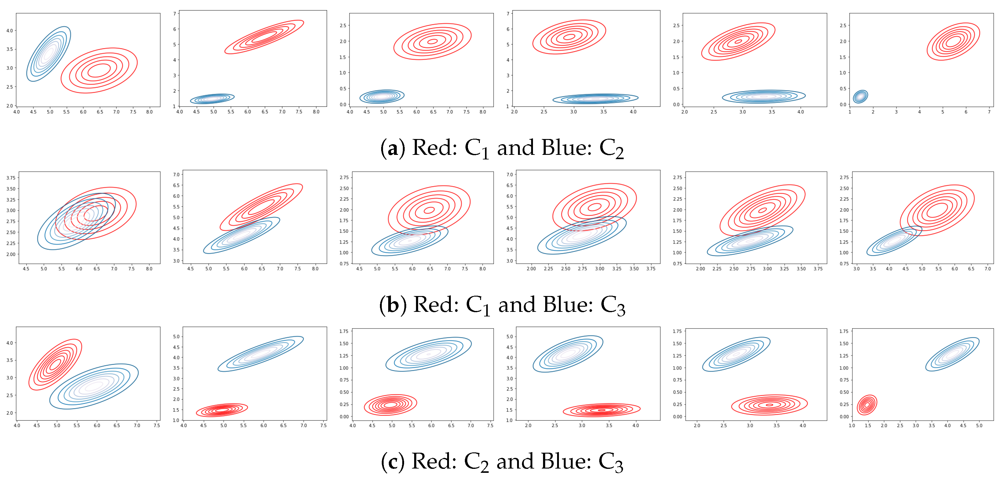
From Table 4 and Figure 2, it is evident that clusters ${\mathrm{C}}_1$ vs. ${\mathrm{C}}_2$ and ${\mathrm{C}}_2$ vs. ${\mathrm{C}}_3$ are substantially differentiated from one another, whereas clusters ${\mathrm{C}}_1$ vs. ${\mathrm{C}}_3$ are not.

Figure 2. $BC$ plot over pairs of features: (${\mathrm{F}}_1$, ${\mathrm{F}}_2$), (${\mathrm{F}}_1$, ${\mathrm{F}}_3$), (${\mathrm{F}}_1$, ${\mathrm{F}}_4$), (${\mathrm{F}}_2$, ${\mathrm{F}}_3$), (${\mathrm{F}}_2$, ${\mathrm{F}}_4$), and (${\mathrm{F}}_3$, ${\mathrm{F}}_4$). Each subfigure represents a pair of clusters of the Iris dataset.

The high rate of overlap between clusters ${\mathrm{C}}_1$ and ${\mathrm{C}}_3$ necessitates an additional round in which three attributes are considered. Table 5 depicts the results of the third round. Sets ${\mathrm{F}}_1$, ${\mathrm{F}}_3$, and ${\mathrm{F}}_4$ offered the lowest $BC$ value, 0.1, making those features the best option for discriminating, although it is greater than 0.05. These numbers are consistent with the Iris cluster analysis literature, as many authors state that the Iris data could be considered 2-cluster data as well as 3-cluster data based on the visual observation of the 2-D projection of the Iris data [40,41].

Table 5. $BC$ values over sets of three features of the Iris dataset.

Features	${\mathbf{F}}_1$, ${\mathbf{F}}_2$, ${\mathbf{F}}_3$	${\mathbf{F}}_1$, ${\mathbf{F}}_2$, ${\mathbf{F}}_4$	${\mathbf{F}}_1$, ${\mathbf{F}}_3$, ${\mathbf{F}}_4$	${\mathbf{F}}_2$, ${\mathbf{F}}_3$, ${\mathbf{F}}_4$
${\mathrm{C}}_1$, ${\mathrm{C}}_3$	0.17	0.24	0.1	0.16

In general, the overlap rate between each pair of clusters is substantially lower than when only a subset of features is considered. Using $BC$ as a reference, features ${\mathrm{F}}_1$, ${\mathrm{F}}_3$, and ${\mathrm{F}}_4$ best distinguish the two clusters.

Iris Global Interpretation

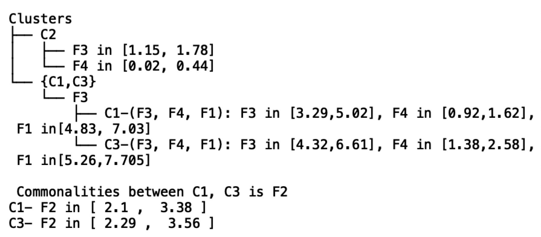
Because cluster ${\mathrm{C}}_2$ is distinguishable from clusters ${\mathrm{C}}_1$ and ${\mathrm{C}}_3$, the algorithm includes it first along with the two distinguishing features listed in order of importance and their domains. The least separable clusters are ${\mathrm{C}}_1$ and ${\mathrm{C}}_3$, which have the best chance of being separated using the set of features ${\mathrm{F}}_3$, ${\mathrm{F}}_4$ and ${\mathrm{F}}_1$. It finally provides the indistinguishable feature ${\mathrm{F}}_2$ (see Figure 3).

Figure 3. Iris dataset global interpretation.

After setting the feature list, the cluster weight is determined using Equations (4) and (5) for each cluster; we obtained the following weights $w_1=0.375$, $w_2=0.6,$ and $w_3=0.025$.

To validate our results, we employe marginalization over features by utilizing Equations (11) and (12). Table 6 displays the results. We can observe that feature ${\mathrm{F}}_2$ has a lesser impact than features ${\mathrm{F}}_3$ and ${\mathrm{F}}_4$. It is essential to note that no changes were made to ${\mathrm{C}}_2$’s assignment because ${\mathrm{C}}_2$ is highly separable by more than one feature (see Table 2), and it has the highest cluster weight.

Table 6. Iris dataset: marginalization over each feature.

	${\mathbf{C}}_1$	${\mathbf{C}}_2$	${\mathbf{C}}_3$
${\mathrm{F}}_1$	$6.6460\times {10}^{-2}$	$2.73\times {10}^{-33}$	$6.6460\times {10}^{-2}$
${\mathrm{F}}_2$	$5.0140\times {10}^{-2}$	$3.78\times {10}^{-31}$	$5.0150\times {10}^{-2}$
${\mathrm{F}}_3$	$7.4690\times {10}^{-2}$	$6.45\times {10}^{-20}$	$7.4691\times {10}^{-2}$
${\mathrm{F}}_4$	$9.3927\times {10}^{-2}$	$8.02\times {10}^{-25}$	$9.3927\times {10}^{-2}$

5.2.2. Swiss Banknote Dataset

There are only two clusters in the data; therefore, there is no need to examine various pairings of clusters; each feature is examined separately. As shown in Table 7, feature ${\mathrm{F}}_6$ (diagonal) has the lowest $BC$, whereas feature ${\mathrm{F}}_1$ (area) has the highest $BC$, exceeding the 0.95 threshold. Thus, it has to be removed from the list of features to be investigated and added to the list of common features.

Table 7. $BC$ values over one feature of the Swiss banknote dataset.

	${\mathbf{F}}_1$	${\mathbf{F}}_2$	${\mathbf{F}}_3$	${\mathbf{F}}_4$	${\mathbf{F}}_5$	${\mathbf{F}}_6$
${\mathrm{C}}_1$, ${\mathrm{C}}_2$	0.98	0.83	0.77	0.4	0.75	0.1

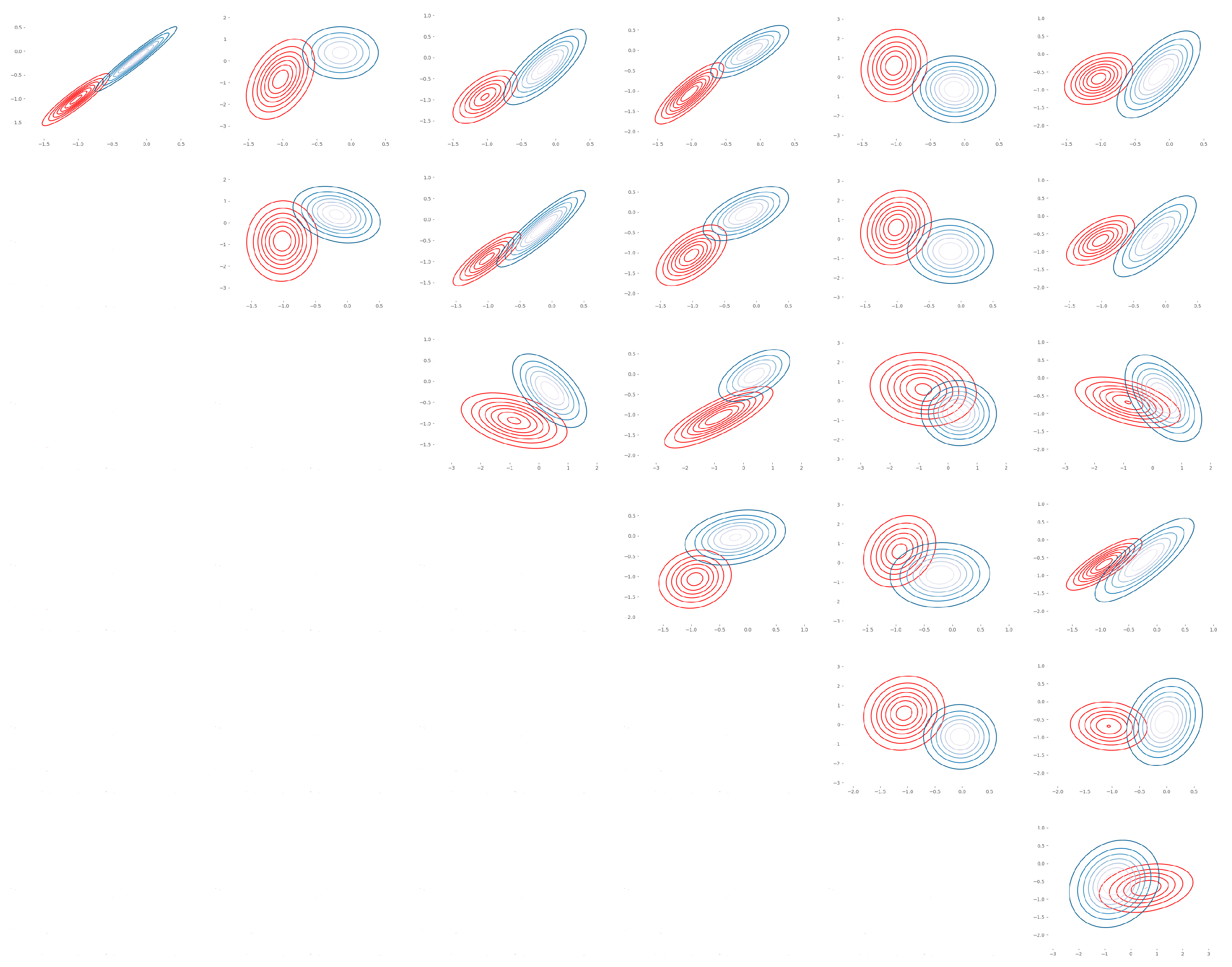
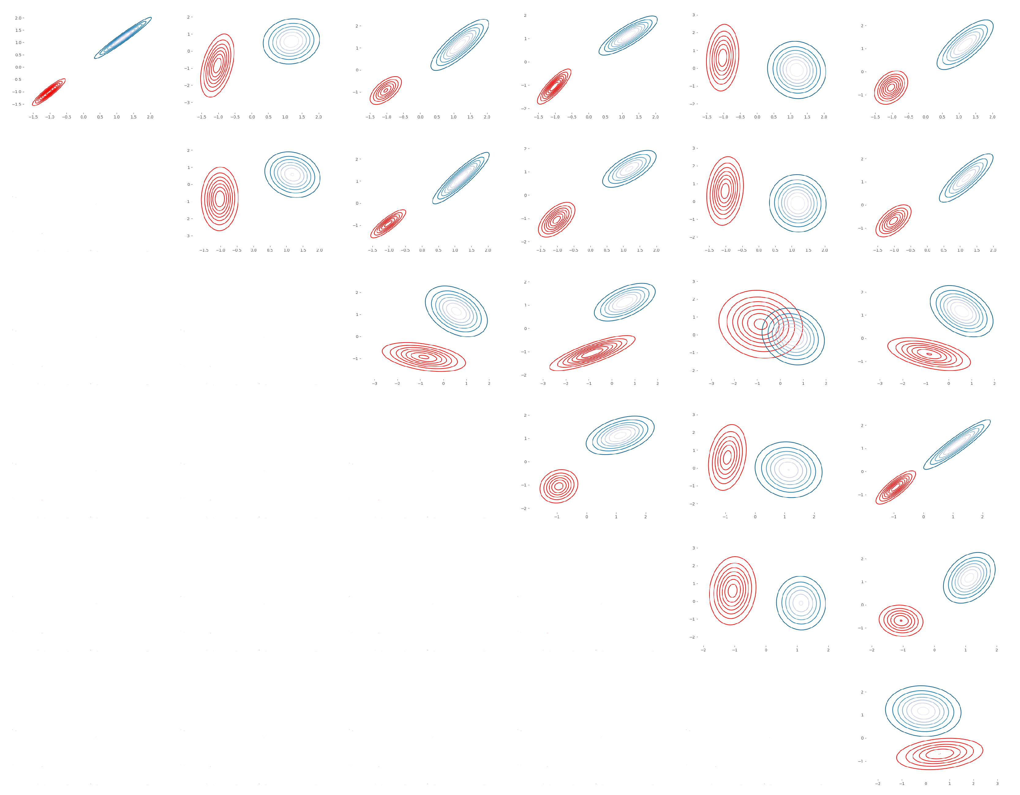
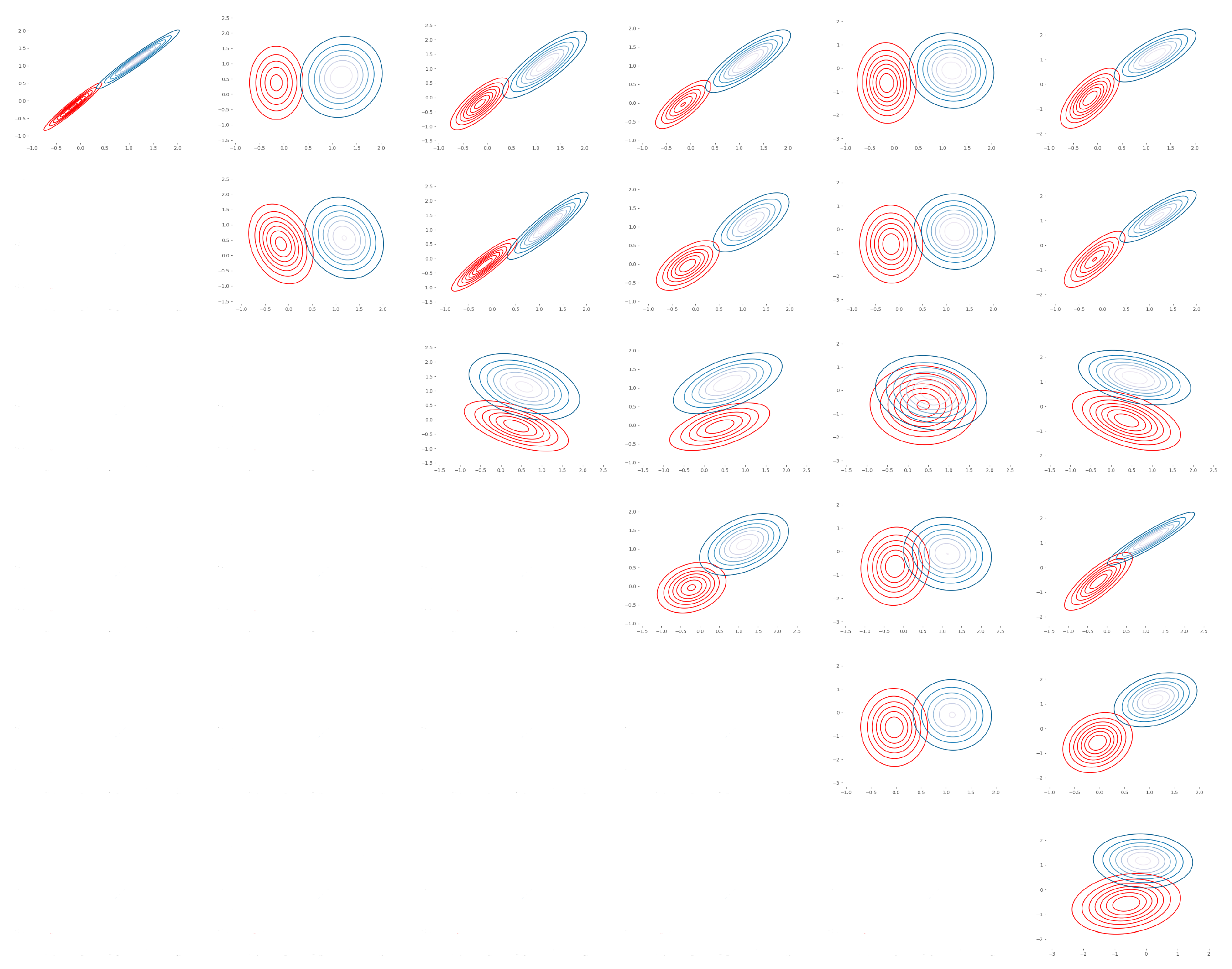
Features ${\mathrm{F}}_1$, ${\mathrm{F}}_2$, and ${\mathrm{F}}_3$ have no influence on the assignment when marginalization is employed (Table 8). Feature ${\mathrm{F}}_4$ has a 1% impact on the probability of assigning 20% of the test instances. The removal of feature ${\mathrm{F}}_5$ decreases the probability of a single instance. Finally, feature ${\mathrm{F}}_6$ prompted a total reversal of two instances and a 50% decrease in a third instance. However, no value is regarded as a distinguishing feature, and another round is necessary for every pair of features.

Table 8. Marginalization over each feature of the Swiss banknote dataset.

	${\mathbf{F}}_1$	${\mathbf{F}}_2$	${\mathbf{F}}_3$	${\mathbf{F}}_4$	${\mathbf{F}}_5$	${\mathbf{F}}_6$
Change	0	0	0	0.0003	0.008059	0.03862

As shown in Table 9, the $BC$ value of the pair of features (${\mathrm{F}}_4$, ${\mathrm{F}}_6$) is less than 0.05, making it a distinguishing pair. Validation using Equation (11) yields 0.13, demonstrating the importance of combining the two features. It is worth noting that we maintain feature ${\mathrm{F}}_1$ to illustrate that retaining features with a high $BC$ value, which does not improve the ability to differentiate clusters (see Table 9).

Table 9. $BC$ values over pair of features of the Swiss banknote dataset.

	${\mathbf{F}}_2$	${\mathbf{F}}_3$	${\mathbf{F}}_4$	${\mathbf{F}}_5$	${\mathbf{F}}_6$
${\mathrm{F}}_1$	0.75	0.70	0.40	0.73	0.100
${\mathrm{F}}_2$		0.73	0.33	0.64	0.090
${\mathrm{F}}_3$			0.30	0.60	0.070
${\mathrm{F}}_4$				0.06	0.017
${\mathrm{F}}_5$					0.089

Cluster ${\mathrm{C}}_1$ weighs 0.416% and Cluster ${\mathrm{C}}_2$ weighs 0.584% of the total clusters weight. Therefore, we are aware that the assignment is mostly dependent on the value of the features.

Swiss Banknote Global Interpretation

The features ${\mathrm{F}}_6$ and ${\mathrm{F}}_4$ are the best to distinguish the two clusters, with a $BC$ value of 0.017. However, the feature ${\mathrm{F}}_1$ is the most indistinguishable between the two distributions with a $BC$ value of 0.98; hence, it is added as a common or similar feature (Figure 4).

Figure 4. Swiss banknote dataset Global Interpretation.

5.2.3. Seeds Dataset

Calculating the $BC$ values for each pair of clusters using a single feature (see Table 10 demonstrates that clusters ${\mathrm{C}}_1$ and ${\mathrm{C}}_3$ are distinguishable with three features (${\mathrm{F}}_1$, ${\mathrm{F}}_2$, and ${\mathrm{F}}_5$). In addition, feature ${\mathrm{F}}_4$ has a very low $BC$; hence, the set of features (${\mathrm{F}}_1$, ${\mathrm{F}}_2$, ${\mathrm{F}}_5$) is the distinguishing list between the clusters ${\mathrm{C}}_1$ and ${\mathrm{C}}_3$. On the other hand, cluster ${\mathrm{C}}_2$ overlapped with the other two, especially with cluster ${\mathrm{C}}_3$, as evidenced by $BC$ values of features ${\mathrm{F}}_3$ and ${\mathrm{F}}_6$ exceeding 0.95. Table 11 shows that when features were removed, cluster ${\mathrm{C}}_2$ changed the most.

Table 10. $BC$ values over one feature of the Seeds dataset.

	${\mathbf{F}}_1$	${\mathbf{F}}_2$	${\mathbf{F}}_3$	${\mathbf{F}}_4$	${\mathbf{F}}_5$	${\mathbf{F}}_6$	${\mathbf{F}}_7$
${\mathrm{C}}_1$, ${\mathrm{C}}_2$	0.280	0.380	0.720	0.650	0.350	0.790	0.930
${\mathrm{C}}_1$, ${\mathrm{C}}_3$	0.006	0.008	0.660	0.080	0.020	0.910	0.120
${\mathrm{C}}_2$, ${\mathrm{C}}_3$	0.190	0.210	0.990	0.410	0.300	0.950	0.310

Table 11. Marginalization over each feature of the Seeds dataset.

	${\mathbf{F}}_1$	${\mathbf{F}}_2$	${\mathbf{F}}_3$	${\mathbf{F}}_4$	${\mathbf{F}}_5$	${\mathbf{F}}_6$	${\mathbf{F}}_7$
${\mathrm{C}}_1$	0.073	0.073	0.065	0.028	0.002	0.004	0.000
${\mathrm{C}}_2$	0.094	0.110	0.085	0.067	0.040	0.040	0.047
${\mathrm{C}}_3$	0.020	0.033	0.020	0.039	0.039	0.039	0.039

Another round is needed over the features in between the ranges of 0.05 and 0.95, namely those for the clusters ${\mathrm{C}}_1$, ${\mathrm{C}}_2$ = {${\mathrm{F}}_1$, ${\mathrm{F}}_2$, ${\mathrm{F}}_3$, ${\mathrm{F}}_4$, ${\mathrm{F}}_5$, ${\mathrm{F}}_6$, ${\mathrm{F}}_7$}, ${\mathrm{C}}_1$, ${\mathrm{C}}_3$ = {${\mathrm{F}}_3$, ${\mathrm{F}}_4$, ${\mathrm{F}}_6$, ${\mathrm{F}}_7$}, and ${\mathrm{C}}_2$, ${\mathrm{C}}_3$ = {${\mathrm{F}}_1$, ${\mathrm{F}}_2$, ${\mathrm{F}}_4$, ${\mathrm{F}}_5$, ${\mathrm{F}}_7$}, (see Appendix A Table A1, Table A2 and Table A3 along with their corresponding Figure A1, Figure A2 and Figure A3). It is evident that retaining features with considerable overlap serves neither cluster ${\mathrm{C}}_2$ nor cluster ${\mathrm{C}}_3$ (see pair of features (${\mathrm{F}}_3$, ${\mathrm{F}}_6$) in Table A3). As a result, it is concluded that considering only two features is insufficient to distinguish cluster ${\mathrm{C}}_2$ from the other clusters. The three features were more effective in differentiating the clusters ${\mathrm{C}}_1$ and ${\mathrm{C}}_2$ when the set of features ${\mathrm{F}}_1$, ${\mathrm{F}}_2$, and ${\mathrm{F}}_3$ was used, but it was still insufficient (more than 0.05). The best set of features to differentiate ${\mathrm{C}}_1$ from ${\mathrm{C}}_2$ are ${\mathrm{F}}_1$, ${\mathrm{F}}_2$, ${\mathrm{F}}_3$, and ${\mathrm{F}}_7$, which allow the least potential overlap between the two clusters ($BC$ = 0.056).

Clearly, the clusters ${\mathrm{C}}_1$ and ${\mathrm{C}}_3$ are distinct from one another, as shown by the plot in Figure A2 with three $BC$ values below 0.05.

Finally, for the clusters ${\mathrm{C}}_2$, ${\mathrm{C}}_3$, after removing features ${\mathrm{F}}_3$ and ${\mathrm{F}}_6$, a combination of features cannot exceed five. The set of four features yields the following values: 0.13, 0.1, 0.12, 0.12, and 0.11. This required the use of five features to distinguish the clusters ${\mathrm{C}}_2$ and ${\mathrm{C}}_3$.

Finally, we calculate the cluster weight using Equations (5) and (6) and obtain the following weights, $w_1=0.7$, $w_2=0.17$, and $w_3=0.13$.

5.3. Local Interpretation

We apply our local interpretation method to the three datasets by selecting instances that exhibit a pattern that cannot be interpreted by features alone.

5.3.1. Iris Dataset

The Mahalanobis distance and the cluster weight are two crucial factors to consider when interpreting the GMM assignment. We selected the first two Iris testing points to be closer to cluster ${\mathrm{C}}_3$ in terms of distance, although cluster ${\mathrm{C}}_1$ has a greater probability due to its greater weight (see Section 5.2.1). The values for each point are listed in Appendix B, listed as iris-1, iris-2, iris-3, and iris-4 (Table A4).

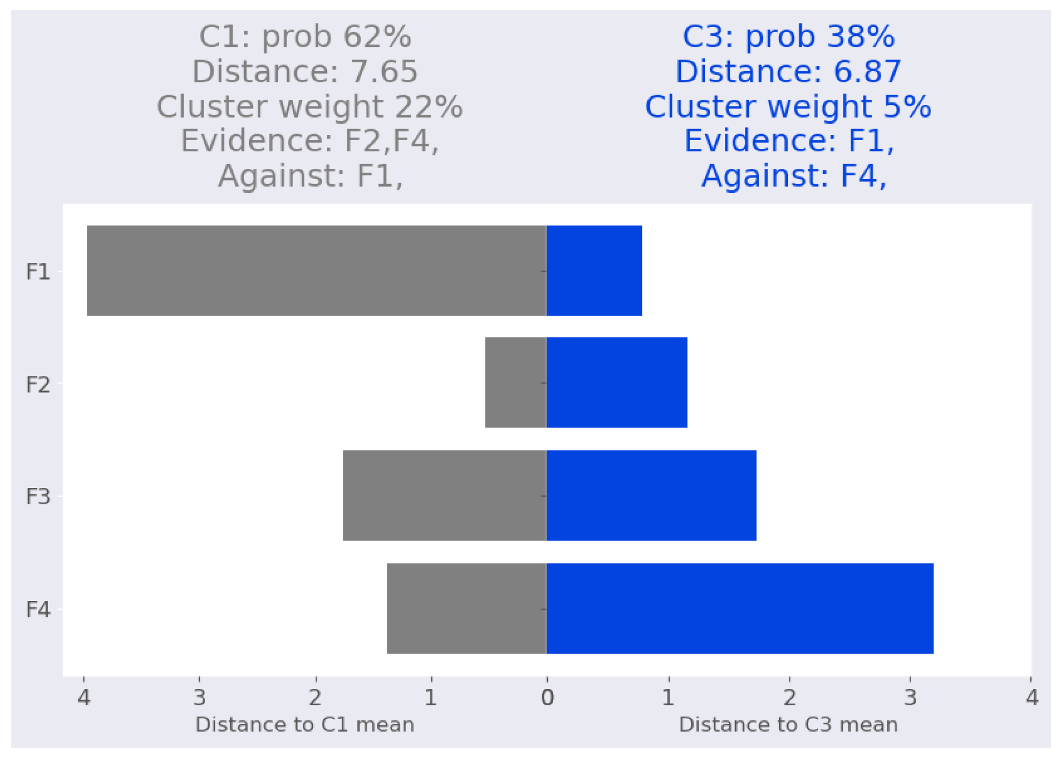
Figure 5 depicts our interpretation of the point iris-1. Notably, iris-1 is closer to cluster ${\mathrm{C}}_3$ than ${\mathrm{C}}_1$, yet ${\mathrm{C}}_1$ is assigned a higher probability due to its higher cluster weight.

Figure 5. Iris dataset: iris-1 local Interpretation.

For the cluster ${\mathrm{C}}_1$, features ${\mathrm{F}}_2$ and ${\mathrm{F}}_4$ provide evidence that supports the cluster assignment while feature ${\mathrm{F}}_1$ does not. This result is supported by Table 12, which demonstrates that eliminating feature ${\mathrm{F}}_2$ reduces the cluster probability from 62% to 46%, while eliminating feature ${\mathrm{F}}_4$ reduces the probability to 22%. In contrast, eliminating feature ${\mathrm{F}}_1$, which does not support the cluster assignment, boosts the probability from 62% to 98% due to its substantial contribution to the cluster mean distance (52%).

Table 12. Validating local interpretation point iris-1. Clu. is the cluster number, Prob: cluster probability, Dist: Mahalanobis distance from the point to the corresponding cluster mean.

Clu.	Prob.	Dist.	${\mathbf{F}}_1$	${\mathbf{F}}_2$	${\mathbf{F}}_3$	${\mathbf{F}}_4$
${\mathrm{C}}_1$	62%	7.65	4.00	0.50	1.75	1.38
${\mathrm{C}}_3$	38%	6.86	0.78	1.15	1.72	3.20
${\mathrm{C}}_1$	98%	1.70	-	0.20	0.03	1.50
${\mathrm{C}}_3$	2%	6.80	-	1.00	2.54	3.20
${\mathrm{C}}_1$	46%	7.23	3.50	-	1.90	1.80
${\mathrm{C}}_3$	54%	4.20	0.50	-	1.90	1.90
${\mathrm{C}}_1$	85%	5.10	2.00	0.60	-	2.50
${\mathrm{C}}_3$	15%	6.70	1.80	1.10	-	3.80
${\mathrm{C}}_1$	22%	7.50	3.80	0.90	2.80	-
${\mathrm{C}}_3$	78%	3.80	0.70	0.30	2.80	-

In terms of the Mahalanobis distance, the point is closer to cluster ${\mathrm{C}}_3$. Feature ${\mathrm{F}}_1$ is the nearest evidence feature, but feature ${\mathrm{F}}_4$ defies the cluster assignment. Eliminating feature ${\mathrm{F}}_1$ on the cluster ${\mathrm{C}}_3$ assignment results in the probability declining from 38% to 2%. As it contributes equally to both clusters (${\mathrm{C}}_1$: 1.75 and ${\mathrm{C}}_3$: 1.72; the difference is minor), feature ${\mathrm{F}}_3$ is neutral and is not counted for either cluster.

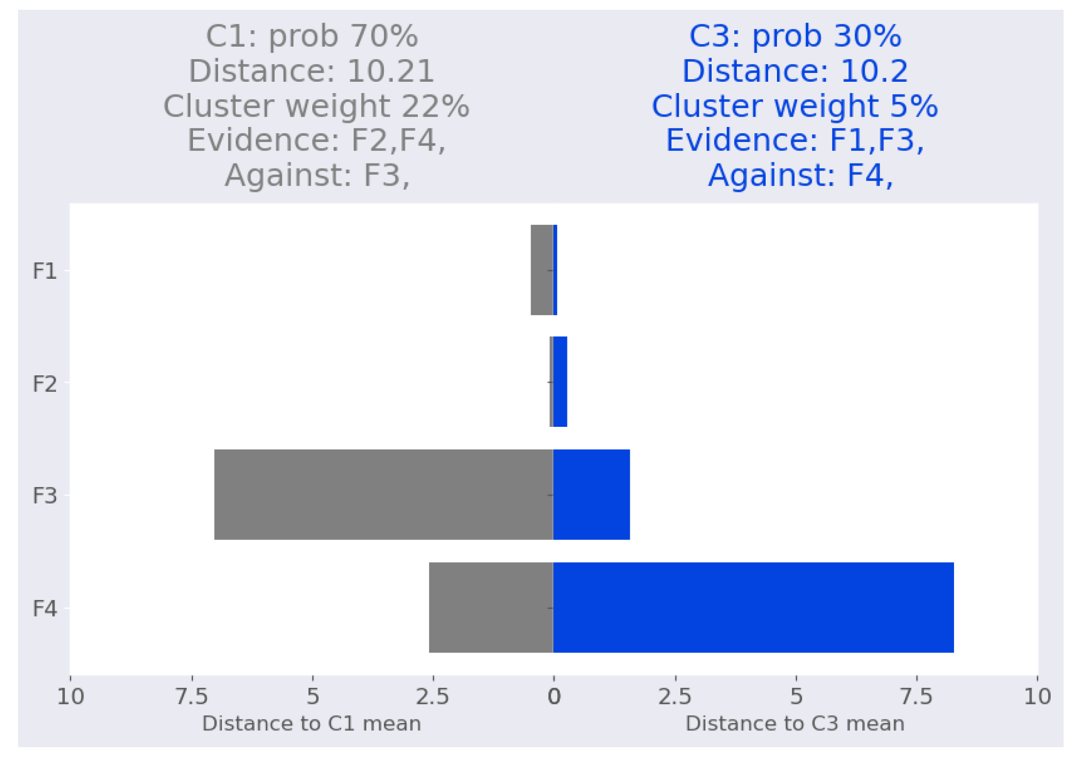
Figure 6 depicts the iris-2 interpretation, which reveals that the distances between iris-2 and the two clusters are approximately equal (10.2 and 10.21). However, GMM assigned a 70% probability to cluster ${\mathrm{C}}_1$ and a 30% probability to cluster ${\mathrm{C}}_3$. This is due to cluster weight rather than impact of the features. For cluster ${\mathrm{C}}_1$, features ${\mathrm{F}}_2$ and ${\mathrm{F}}_4$ represent the evidence, and their removal reduces the likelihood to 69% and 62%, respectively, as shown in Table 13. In contrast, feature ${\mathrm{F}}_3$ is considered to be against the cluster assignment, and eliminating it boosts the cluster probability from 70% to 99.5%.

Figure 6. Iris dataset: iris-2 local interpretation.

Table 13. Validating local interpretation point iris-2. Clu. is the cluster number, Prob: cluster probability, Dist: Mahalanobis distance from the point to the corresponding cluster mean.

Clu	Prob.	Dist.	${\mathbf{F}}_1$	${\mathbf{F}}_2$	${\mathbf{F}}_3$	${\mathbf{F}}_4$
${\mathrm{C}}_1$	70.0%	10.21	0.50	0.10	7.04	2.6
${\mathrm{C}}_3$	30.0%	10.20	0.08	0.30	1.57	8.3
${\mathrm{C}}_1$	94.4%	6.60	-	0.03	4.20	2.4
${\mathrm{C}}_3$	5.6%	9.60	-	0.30	0.90	8.4
${\mathrm{C}}_1$	69.0%	9.80	0.40	-	7.10	2.3
${\mathrm{C}}_3$	31.0%	8.55	0.18	-	1.70	6.7
${\mathrm{C}}_1$	99.5%	0.96	0.22	0.14	-	0.6
${\mathrm{C}}_3$	0.5%	9.50	0.07	0.30	-	9.1
${\mathrm{C}}_1$	62.0%	3.75	0.40	0.01	3.30	-
${\mathrm{C}}_3$	38.0%	3.50	0.14	0.08	3.30	-

In other cases, the Mahalanobis distance between the point and higher probability cluster is smaller than the distance between the point and the lesser probability cluster. This is demonstrated in iris-3 (Figure 7) where all features are closer to cluster ${\mathrm{C}}_1$ rather than ${\mathrm{C}}_3$.

Figure 7. Iris dataset: iris-3 local interpretation.

As shown in Table 14, marginalizing over a single feature never flips the assignment or reduces it by more than 8%.

Table 14. Iris dataset: validating local interpretation point iris-3. Clu. is the cluster number, Prob: cluster probability, Dist: Mahalanobis distance from the point to the corresponding cluster mean.

Clu	Prob.	Dist.	${\mathbf{F}}_1$	${\mathbf{F}}_2$	${\mathbf{F}}_3$	${\mathbf{F}}_4$
${\mathrm{C}}_1$	98.0%	4.64	0.120	1.97	0.42	2.12
${\mathrm{C}}_3$	2.0%	11.01	0.420	3.80	3.70	3.10
${\mathrm{C}}_1$	98.1%	4.10	-	1.80	0.09	2.19
${\mathrm{C}}_3$	1.9%	9.30	-	4.13	1.90	3.30
${\mathrm{C}}_1$	93.0%	3.70	0.023	-	0.54	3.11
${\mathrm{C}}_3$	7.0%	6.06	0.920	-	3.90	1.23
${\mathrm{C}}_1$	94.0%	4.60	0.040	2.06	-	2.50
${\mathrm{C}}_3$	6.0%	8.01	0.100	3.80	-	4.10
${\mathrm{C}}_1$	92.0%	4.02	0.095	2.70	1.20	-
${\mathrm{C}}_3$	8.0%	7.80	0.530	1.97	5.30	-

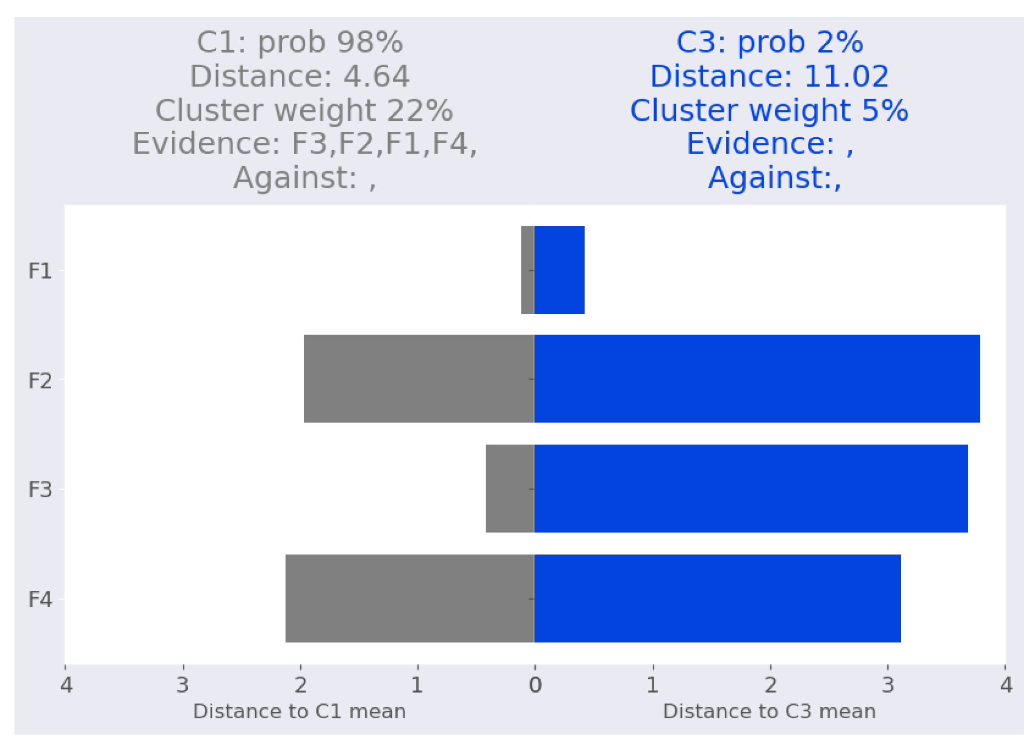
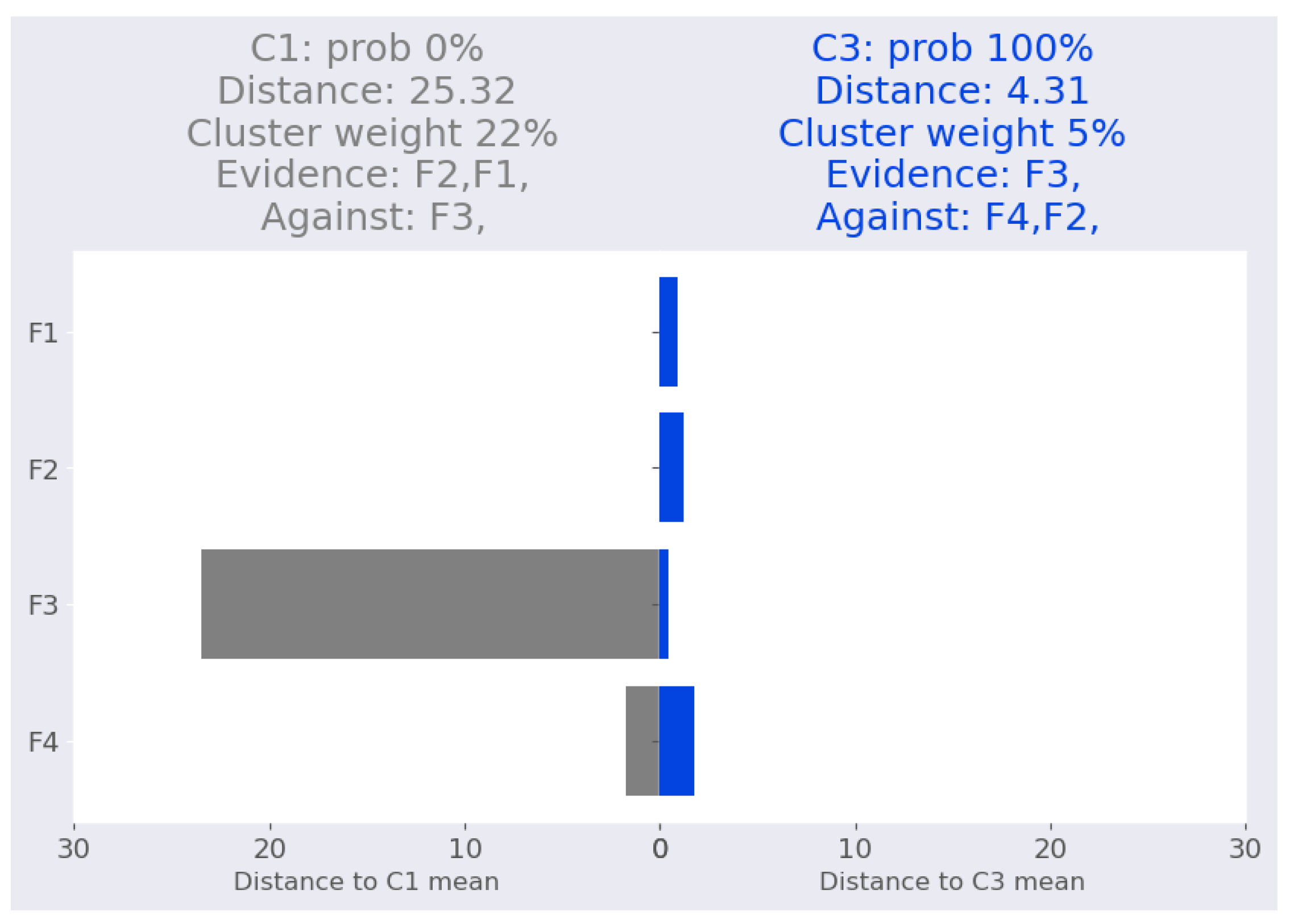
The last point is iris-4. GMM is 100 percent certain that it belongs to the cluster ${\mathrm{C}}_3$. The distances between iris-4 and the two closest clusters are vastly different. According to our interpretation, which is shown in Figure 8, the evidence for the cluster ${\mathrm{C}}_3$ comes from feature ${\mathrm{F}}_3$. This is confirmed by Table 15. On the other hand, feature ${\mathrm{F}}_4$ contributes equally to both clusters, while features ${\mathrm{F}}_1$ and ${\mathrm{F}}_2$ are more closely related to the cluster ${\mathrm{C}}_1$.

Figure 8. Iris dataset: iris-4 local interpretation.

Table 15. Validating local interpretation point iris-4. Clu. is the cluster number, Prob: cluster probability, Dist: Mahalanobis distance from the point to the corresponding cluster mean.

Clu.	Prob.	Dist.	${\mathbf{F}}_1$	${\mathbf{F}}_2$	${\mathbf{F}}_3$	${\mathbf{F}}_4$
${\mathrm{C}}_1$	0%	25.30	0.040	0.002	23.50	1.80
${\mathrm{C}}_3$	100%	4.30	0.900	1.200	0.46	1.76
${\mathrm{C}}_1$	1%	19.20	-	0.004	17.10	2.16
${\mathrm{C}}_3$	99%	4.19	-	1.350	1.10	1.70
${\mathrm{C}}_1$	0%	25.00	0.070	-	23.50	1.46
${\mathrm{C}}_3$	100%	2.60	1.240	-	0.40	0.94
${\mathrm{C}}_1$	16%	9.50	2.500	0.050	-	6.95
${\mathrm{C}}_3$	84%	4.20	1.400	1.200	-	1.60
${\mathrm{C}}_1$	0%	24.85	0.005	0.030	24.80	-
${\mathrm{C}}_3$	100%	1.58	1.030	0.420	0.13	-

Finally, Table 16 displays local metrics across the three points (for iris-3, the models select all features). The drop in probability in the comprehensiveness column indicates that the correct features were selected. Furthermore, none of the values in the sufficiency column were negative, so retaining these features helped increase, or at the very least maintained, confidence in the model’s original prediction.

Table 16. Iris dataset: local interpretability metrics.

Point	Original Prediction	Comprehensiveness	Sufficiency
iris-1	${\mathrm{C}}_1$: 62%	${\mathrm{C}}_1$: 25% (37%)	${\mathrm{C}}_1$: 93% (31%)
iris-2	${\mathrm{C}}_1$: 70%	${\mathrm{C}}_1$: 66% (4%)	${\mathrm{C}}_1$: 99.5% (29.5%)
iris-4	${\mathrm{C}}_3$: 100%	${\mathrm{C}}_3$: 81% (19%)	${\mathrm{C}}_3$: 100% (0%)

5.3.2. Swiss Banknote Dataset

For the Swiss banknote, the model has a high degree of confidence in the assignment of the test data evidenced by all of the selected points belonging one hundred percent to the cluster. The values of the selected points are listed in Appendix B, (Table A5).

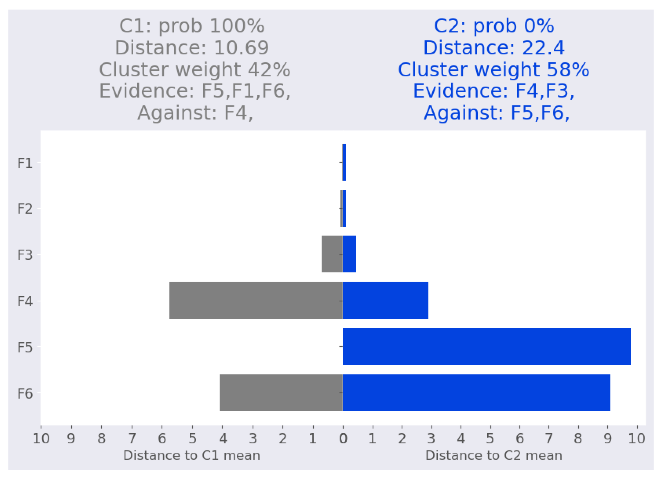
For the first point swiss-1, the instance is assigned with absolute confidence to the cluster ${\mathrm{C}}_1$ due to the similarities of features ${\mathrm{F}}_5$, ${\mathrm{F}}_1$, and ${\mathrm{F}}_6$ (Figure 9). Cluster ${\mathrm{C}}_2$ is supported by features ${\mathrm{F}}_4$ and ${\mathrm{F}}_3$.

Figure 9. Swiss banknote dataset: Swiss-1 local interpretation.

We validated this interpretation by removing features ${\mathrm{F}}_5$ and ${\mathrm{F}}_6$ to determine their effect on the cluster assignment probability. As shown in Table 17, the distance from cluster ${\mathrm{C}}_1$ decreased from 10.7 to 3.11, while the distance from cluster ${\mathrm{C}}_2$ decreased from 22.4 to 2.2, resulting in the probability of cluster ${\mathrm{C}}_2$ increasing from 0% to 61%. Table 18 shows that the largest decline induced by a single feature is obtained when feature ${\mathrm{F}}_5$ is removed.

Table 17. Validating local interpretation point swiss-1 after removing two features (${\mathrm{F}}_5$, ${\mathrm{F}}_6$). Clu. is the cluster number, Prob: cluster probability, Dist: Mahalanobis distance from the point to the corresponding cluster mean.

Clu.	Prob.	Dist.	${\mathbf{F}}_1$	${\mathbf{F}}_2$	${\mathbf{F}}_3$	${\mathbf{F}}_4$	${\mathbf{F}}_5$	${\mathbf{F}}_6$
${\mathrm{C}}_1$	100%	10.70	0.0500	0.100	0.70	5.80	0.0002	4.07
${\mathrm{C}}_2$	0%	22.40	0.1000	0.080	0.40	2.88	9.8000	9.10
${\mathrm{C}}_1$	39%	3.11	0.0005	0.014	0.18	2.90	-	-
${\mathrm{C}}_2$	61%	2.20	0.3400	0.500	0.95	0.40	-	-

Table 18. Validating local interpretation point swiss-1. Clu. is the cluster number, Prob: cluster probability, Dist: Mahalanobis distance from the point to the corresponding cluster mean.

Clu.	Prob.	Dist.	${\mathbf{F}}_1$	${\mathbf{F}}_2$	${\mathbf{F}}_3$	${\mathbf{F}}_4$	${\mathbf{F}}_5$	${\mathbf{F}}_6$
${\mathrm{C}}_1$	100.0%	10.70	0.0500	0.1000	0.70	5.80	0.0002	4.07
${\mathrm{C}}_2$	0.0%	22.40	0.1000	0.0800	0.40	2.88	9.8000	9.10
${\mathrm{C}}_1$	99.7%	10.01	-	0.0500	0.70	5.40	0.0020	3.90
${\mathrm{C}}_2$	0.3%	22.30	-	0.1200	0.40	2.80	9.8000	9.30
${\mathrm{C}}_1$	98.9%	10.13	0.0200	-	0.50	5.70	0.0002	3.90
${\mathrm{C}}_2$	1.1%	20.50	0.1600	-	0.19	2.60	9.0400	8.70
${\mathrm{C}}_1$	99.8%	8.70	0.0400	0.0034	-	5.26	0.0008	3.40
${\mathrm{C}}_2$	0.2%	22.30	0.0700	0.0300	-	3.04	10.0000	9.15
${\mathrm{C}}_1$	99.8%	3.50	0.0070	0.0900	0.40	-	0.9000	2.10
${\mathrm{C}}_2$	0.2%	16.20	0.0200	0.0015	0.73	-	5.7000	9.70
${\mathrm{C}}_1$	68.0%	9.40	0.0300	0.1200	0.70	4.80	-	3.80
${\mathrm{C}}_2$	32.0%	11.40	0.0600	0.0400	0.80	0.30	-	10.15
${\mathrm{C}}_1$	99.7%	3.20	0.0004	0.0140	0.17	2.90	0.1100	-
${\mathrm{C}}_2$	0.3%	15.40	0.4000	0.0170	0.50	3.50	11.0000	-

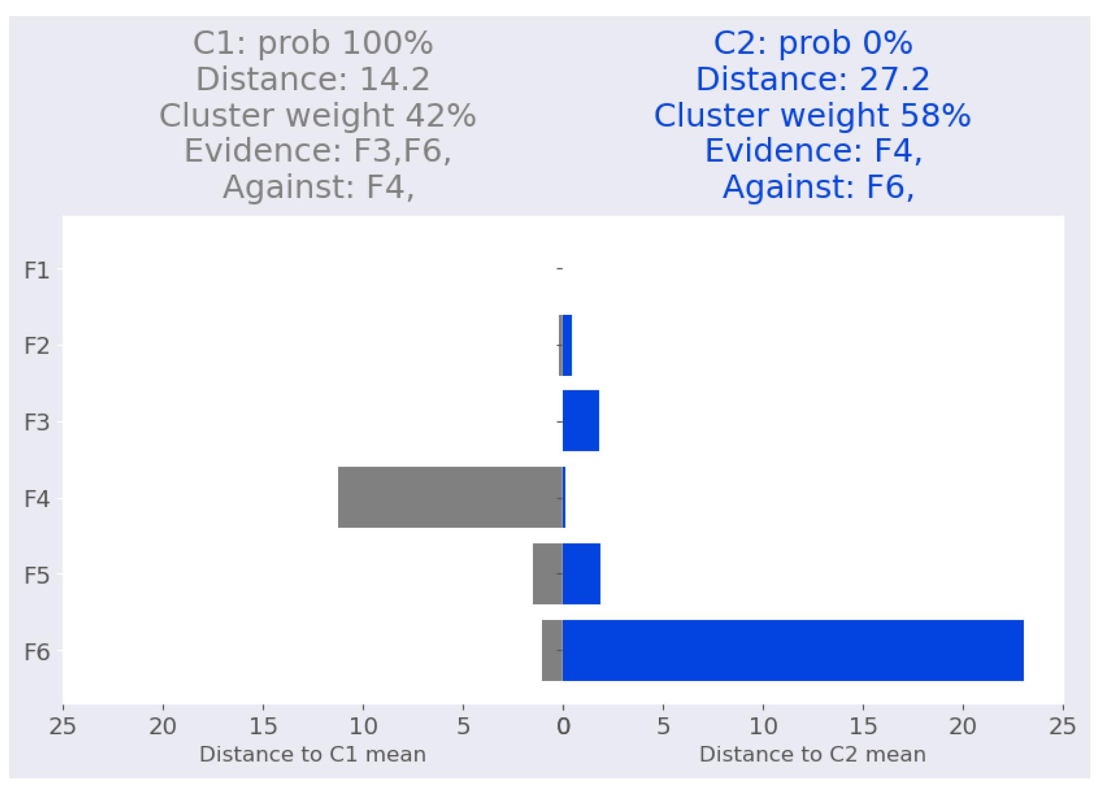
The second point interpretation is depicted in Figure 10, with absolute certainty that this point belongs to cluster ${\mathrm{C}}_1$ based on features ${\mathrm{F}}_3$ and ${\mathrm{F}}_6$ as an evidence and feature ${\mathrm{F}}_4$ as opposition. When the two evidence features are eliminated, the assignment yielded a 97% certainty that this point belongs to cluster ${\mathrm{C}}_2$, as shown in Table 19. Moreover, when examining the impact of removing each feature individually (Table 20), we observe that the feature ${\mathrm{F}}_6$ has the greatest influence due to its large distance from the mean of cluster ${\mathrm{C}}_2$.

Figure 10. Swiss banknote dataset: Swiss-2 local interpretation.

Table 19. Validating local interpretation point swiss-2 after removing two features (${\mathrm{F}}_3$, ${\mathrm{F}}_6$). Prob: cluster probability, Clu. is the cluster number, Dist: Mahalanobis distance from the point to the corresponding cluster mean.

Clu.	Prob.	Dist.	${\mathbf{F}}_1$	${\mathbf{F}}_2$	${\mathbf{F}}_3$	${\mathbf{F}}_4$	${\mathbf{F}}_5$	${\mathbf{F}}_6$
${\mathrm{C}}_1$	100%	14.2	0.0300	0.25	0.012	11.300	1.5	1.1
${\mathrm{C}}_2$	0%	27.2	0.0009	0.40	1.800	0.120	1.9	23.1
${\mathrm{C}}_1$	3%	9.8	0.0010	0.30	-	8.500	1	-
${\mathrm{C}}_2$	97%	3.5	0.1000	0.20	-	0.003	3.2	-

Table 20. Validating local interpretation point swiss-2. Clu. is the cluster number, Prob: cluster probability, Dist: Mahalanobis distance from the point to the corresponding cluster mean.

Clu.	Prob.	Dist.	${\mathbf{F}}_1$	${\mathbf{F}}_2$	${\mathbf{F}}_3$	${\mathbf{F}}_4$	${\mathbf{F}}_5$	${\mathbf{F}}_6$
${\mathrm{C}}_1$	100.0%	14.20	0.03000	0.250	0.012	11.300	1.500	1.10
${\mathrm{C}}_2$	0.0%	27.20	0.00090	0.400	1.800	0.120	1.900	23.10
${\mathrm{C}}_1$	99.8%	13.60	-	0.340	0.009	10.800	1.500	1.00
${\mathrm{C}}_2$	0.2%	27.04	-	0.370	1.800	0.100	1.900	22.80
${\mathrm{C}}_1$	99.0%	14.00	0.07000	-	0.080	11.300	1.500	1.12
${\mathrm{C}}_2$	1.0%	24.60	0.00980	-	1.100	0.200	1.400	21.90
${\mathrm{C}}_1$	99.5%	14.00	0.03000	0.330	-	11.120	1.500	1.00
${\mathrm{C}}_2$	0.5%	25.52	0.03000	0.060	-	0.050	2.150	23.20
${\mathrm{C}}_1$	100.0%	0.42	0.06000	0.300	0.030	-	0.006	0.05
${\mathrm{C}}_2$	0.0%	27.20	0.00004	0.400	1.700	-	2.120	22.94
${\mathrm{C}}_1$	100.0%	7.40	0.00800	0.150	0.007	6.600	-	0.64
${\mathrm{C}}_2$	0.0%	26.44	0.00340	0.200	2.000	0.600	-	23.70
${\mathrm{C}}_1$	7.0%	9.93	0.00200	0.400	0.020	8.500	1.100	-
${\mathrm{C}}_2$	93.0%	5.10	0.25000	0.006	1.980	0.005	2.800	-

Finally, Table 21 displays local metrics for the two points. We can see the high drop in probability in the comprehensiveness column, indicating that the correct features were selected. Furthermore, none of the values in the sufficiency column were negative, thus maintaining the same level of confidence for the model.

Table 21. Swiss banknote dataset: local interpretability metrics.

Point	Original Prediction	Comprehensiveness	Sufficiency
Swiss-1	${\mathrm{C}}_1$: 100%	${\mathrm{C}}_1$: 30% (70%)	${\mathrm{C}}_1$: 100% (0%)
Swiss-2	${\mathrm{C}}_1$: 100%	${\mathrm{C}}_1$: 12% (88%)	${\mathrm{C}}_3$: 100% (0%)

5.3.3. Seeds Dataset

The correlation between features ${\mathrm{F}}_1$ and ${\mathrm{F}}_2$ in the cluster ${\mathrm{C}}_2$ is 0.97. They are highly correlated, and their values are used to calculate the feature ${\mathrm{F}}_3$. We select an instance that demonstrates the significance of resolving the correlation. The sample is assigned to the cluster ${\mathrm{C}}_1$ with a certainty of 72%. The contribution of feature ${\mathrm{F}}_2$ to the total distance from the mean of cluster ${\mathrm{C}}_2$ is 11.3. When feature ${\mathrm{F}}_1$ is removed, this contribution decreases to 1.7. The model cannot identify the contribution of each of the correlated features (see Table 22).

Table 22. Validating local interpretation point seed-1. Clu. is the cluster number, Prob: cluster probability, Dist: Mahalanobis distance from the point to the corresponding cluster mean.

Clu.	Prob.	Dist.	${\mathbf{F}}_1$	${\mathbf{F}}_2$	${\mathbf{F}}_3$	${\mathbf{F}}_4$	${\mathbf{F}}_5$	${\mathbf{F}}_6$	${\mathbf{F}}_7$
${\mathrm{C}}_1$	72.0%	21.50	2.20	0.050	0.1000	8.27	0.00200	2.300	8.60
${\mathrm{C}}_2$	28.0%	20.60	1.50	11.300	5.9000	0.08	1.30000	0.025	0.53
${\mathrm{C}}_1$	0.5%	19.94	-	0.360	0.0002	8.75	0.03700	2.300	8.50
${\mathrm{C}}_2$	99.5%	7.44	-	1.700	3.5000	0.12	1.50000	0.020	0.63
${\mathrm{C}}_1$	0.5%	19.80	0.33	-	0.0014	8.90	0.01700	2.300	8.30
${\mathrm{C}}_2$	99.5%	7.15	1.70	-	3.0000	0.20	1.50000	0.030	0.65
${\mathrm{C}}_1$	0.3%	20.10	0.70	0.090	-	8.50	0.00005	2.300	8.50
${\mathrm{C}}_2$	97.0%	6.10	2.10	0.400	-	0.10	3.20000	0.050	0.30
${\mathrm{C}}_1$	98.0%	15.20	6.30	0.200	1.5000	-	0.00500	2.000	5.10
${\mathrm{C}}_2$	2.0%	20.34	1.30	11.500	5.7000	-	1.30000	0.030	0.60
${\mathrm{C}}_1$	65.0%	21.20	1.80	0.030	0.1400	8.30	-	2.300	8.60
${\mathrm{C}}_2$	35.0%	20.50	1.14	12.000	6.7000	0.10	-	0.020	2.70
${\mathrm{C}}_1$	86.0%	18.90	2.05	0.007	0.0005	7.32	0.17000	-	9.36
${\mathrm{C}}_2$	14.0%	19.50	1.20	10.600	5.8000	0.08	1.26000	-	0.55
${\mathrm{C}}_1$	99.9%	6.80	1.70	0.100	0.0080	2.08	0.06000	2.800	-
${\mathrm{C}}_2$	0.1%	20.30	1.20	12.200	5.5000	0.17	1.20000	0.050	-

It is essential to note that the instance is incorrectly assigned to cluster ${\mathrm{C}}_1$, and should instead be placed in ${\mathrm{C}}_2$. However, correlated features are a prevalent problem that has been addressed using a variety of strategies, such as modifying the model architecture and even the dataset [42] or eliminating redundant neurons from neural networks [43]. One strategy that might be taken to remedy this issue is to remove correlated features and then retrain the model. Table 23 demonstrates that removing the area and perimeter features helps to resolve this issue and improves the model’s overall performance.

Table 23. Validating local interpretation point seed-1 after removing ${\mathrm{F}}_1$ and ${\mathrm{F}}_2$ and retrain the model. Clu. is the cluster number, Prob: cluster probability, Dist: Mahalanobis distance from the point to the corresponding cluster mean.

Clu.	Prob.	Dist.	${\mathbf{F}}_3$	${\mathbf{F}}_4$	${\mathbf{F}}_5$	${\mathbf{F}}_6$	${\mathbf{F}}_7$
${\mathrm{C}}_1$	0.01%	31.80	0.650	12.400000	1.8000	2.400	14.550
${\mathrm{C}}_2$	99.99%	5.00	2.200	0.200000	1.1000	0.080	1.400
${\mathrm{C}}_1$	0.01%	26.30	-	10.000000	0.3000	2.500	13.500
${\mathrm{C}}_2$	99.99%	4.60	-	0.000001	3.4000	0.004	1.100
${\mathrm{C}}_1$	20.00%	8.10	1.800	-	0.6000	1.900	3.800
${\mathrm{C}}_2$	80.00%	5.00	2.200	-	1.2000	0.090	1.500
${\mathrm{C}}_1$	0.01%	24.10	0.300	8.600000	-	2.700	12.500
${\mathrm{C}}_2$	99.99%	5.00	2.800	0.380000	-	0.100	1.800
${\mathrm{C}}_1$	0.01%	30.20	1.200	11.500000	2.9000	-	14.600
${\mathrm{C}}_2$	99.99%	5.00	2.100	0.190000	1.2000	-	1.500
${\mathrm{C}}_1$	63.00%	4.00	0.100	1.500000	0.0002	2.400	-
${\mathrm{C}}_2$	37.00%	4.60	2.000	0.800000	1.6400	0.120	-

5.4. Comparisons with LIME

Since none of the related model-specific work provides a local interpretation, we compare our local interpretation to model-agnostic LIME [9]. Despite being model-agnostic, LIME requires the availability of training data in the case of tabular data.

LIME calculates the mean and standard deviation for each feature of the tabular data and then discretizes them into quartiles to sample around the instance of interest. Since the approximation of the black-box model is dependent on the data, the interpretation is in some way misleading.

5.4.1. Iris Dataset

LIME is a stochastic model in the sense that it generates slightly different output per run. Therefore, we run LIME multiple times and select the most repeated samples. LIME generates two interpretations for the point iris-1 as shown in Figure 11 and Figure 12, LIME regards features ${\mathrm{F}}_4$, ${\mathrm{F}}_3$, and ${\mathrm{F}}_2$ as evidence favoring the cluster assignment for cluster ${\mathrm{C}}_1$, however feature ${\mathrm{F}}_1$ is considered against. According to LIME’s alternative interpretation of cluster ${\mathrm{C}}_1$, features ${\mathrm{F}}_4$ and ${\mathrm{F}}_3$ constitute evidence, but ${\mathrm{F}}_1$ and ${\mathrm{F}}_2$ are against. However, Table 12, show that removing feature ${\mathrm{F}}_3$ (which is intended to be evidence) increases the assignment probability from 62% to 85%; therefore, it cannot be considered an evidence feature if its removal increases the assignment. Due to its location at the same distance from both clusters, ${\mathrm{F}}_3$ neither supports nor opposes the assignment.

Figure 11. LIME interpretation for point iris-1 (sample-1).

Figure 12. LIME interpretation for point iris-1 (sample-2).

For cluster ${\mathrm{C}}_3$, LIME outputs features ${\mathrm{F}}_3$, ${\mathrm{F}}_1$, ${\mathrm{F}}_4$, and ${\mathrm{F}}_2$ as evidence of the assignment, whereas the other interpretation provides features ${\mathrm{F}}_3$, ${\mathrm{F}}_4$, and ${\mathrm{F}}_1$ as evidence of the assignment and ${\mathrm{F}}_2$ is considered against.

However, removing feature ${\mathrm{F}}_4$ causes a drop in the distance between the point and the cluster mean from 6.86 to 3.8, and the assignment probability increases from 38% to 78%. Therefore, ${\mathrm{F}}_4$ is against the assignment of the point to cluster ${\mathrm{C}}_3$, which contradicts LIME. Our method, on the other hand, produces a consistent interpretation and is able to identify the correct set of features.

For the iris-2 point, LIME outputs features ${\mathrm{F}}_4$, ${\mathrm{F}}_3$, and ${\mathrm{F}}_1$ as an evidence of the assignment for cluster ${\mathrm{C}}_1$ (Figure 13). However, removing ${\mathrm{F}}_1$ increases the cluster probability from 70% to 94.4%, while removing ${\mathrm{F}}_3$ increases the cluster probability to 99.5%. ${\mathrm{F}}_2$, however, is considered against the cluster. If we remove ${\mathrm{F}}_2$, the cluster probability decreased by 1%.

Figure 13. LIME interpretation for point iris-2.

LIME considers ${\mathrm{F}}_3$ and ${\mathrm{F}}_2$ as evidence of ${\mathrm{C}}_3$. Removing ${\mathrm{F}}_2$ causes an increase in cluster probability by 1%, while ${\mathrm{F}}_1$ is counted against ${\mathrm{C}}_3$. Indeed, eliminating ${\mathrm{F}}_1$ reduces the cluster’s probability from 30% to 5%.

LIME suggests two interpretations for the instance iris-3, as shown by Figure 14 and Figure 15. Both interpretations agree over features ${\mathrm{F}}_1$, ${\mathrm{F}}_3$, and ${\mathrm{F}}_4$ as evidence. However, ${\mathrm{F}}_3$ and ${\mathrm{F}}_2$ cannot be used as evidence for cluster ${\mathrm{C}}_3$ since their contribution to both distances, and their impact when they are removed are inconsistent with this claim (see Table 14).

Figure 14. LIME interpretation for point iris-3 (sample-1).

Figure 15. LIME interpretation for point iris-3 (sample-2).

Figure 16 shows LIME’s interpretation for the instance iris-4 where it considers feature ${\mathrm{F}}_2$ as supporting the cluster ${\mathrm{C}}_3$ assignment. This contradicts its impact when it is removed to lower the overall distance from 4.3 to 2.6. However, there is no effect on the distance to cluster ${\mathrm{C}}_1$ (see Table 15).

Figure 16. LIME explanation for point iris-4.

5.4.2. Swiss Banknote Dataset

Figure 17 and Figure 18 show that LIME agrees with our interpretation presented in Figure 9, specifically that features ${\mathrm{F}}_5$ and ${\mathrm{F}}_6$ constitute evidence. LIME also deems feature ${\mathrm{F}}_4$ to be evidence, even though it contradicts cluster ${\mathrm{C}}_1$ and supports the other cluster, as shown in Table 18.

Figure 17. LIME explanation for point swiss-1 (sample-1).

Figure 18. LIME explanation for point swiss-1 (sample-2).

LIME selects features ${\mathrm{F}}_6$, ${\mathrm{F}}_4$, ${\mathrm{F}}_5$, and ${\mathrm{F}}_3$ as evidence of the cluster assignment for the point swiss-2, as shown in Figure 19. Table 20 reveals that feature ${\mathrm{F}}_4$ is the most remote feature from the mean of cluster ${\mathrm{C}}_1$. Eliminating this feature decreases the overall distance from 14.2 to 0.42. Therefore, ${\mathrm{F}}_4$ would never be considered as proof of the ${\mathrm{C}}_1$ assignment.

Figure 19. LIME explanation for point swiss-2.

The simplicity of an interpretation and its comprehensiveness are two important factors to consider. The majority of approaches make a trade-off between these two factors, whereas feature-based approaches can attain the optimal balance [44]. Our method can quantify the degree of influence of each feature in a simple and concise way. The corr-max transformation provides an estimate of each feature’s contribution to a quadratic form where the necessary matrices are readily determined. It is a consistent method since, given the same model and input, it always returns the same interpretation. In addition, the interpretation is intrinsic and never compromises accuracy, and we test it in a cost-effective manner compared to other methods, and it avoids the out-of-distribution problem [45]. However, strongly correlated features are a typical issue that hinders the capacity of the approach to define the role of each of the correlated features. Our method is susceptible to this issue.

Interpretation must reflect the logic of a model, and a blind test performed by a model-agnostic to build an equivalent model is not adequate to show the reasoning as the logical equivalence of models is not implied by their output being equivalent.

6. Conclusions

We developed an approach to intrinsically interpret GMM on global and local scales. Our approach provides a global perspective by identifying distinguishing and overlapping features to determine the characteristics of clusters along with cluster weights. Locally, our approach quantifies the features’ contributions to the overall distance from the cluster means. Because it lacks a global perspective, local interpretation fails to represent the real behavior of the model on occasion. To prevent this, we considered global weight while providing local interpretation. Our approach is able to find a precise interpretation while preserving accuracy and model assumptions. The global interpretation is determined by utilizing overlap to identify distinguishing features across clusters, whereas the local interpretation utilizes the corr-max transformation to determine the precise contribution of each feature per instance, in addition to incorporating cluster weights. There are a variety of methods that alter the model to provide an interpretation but affect the accuracy or assumptions. In comparison, our solution maintained the original model’s logic and accuracy.

However, in the case of strongly correlated features, it is difficult to determine the relative importance of each feature; hence, this situation should be noted when interpreting the cluster assignment. In the future, we will address this issue for a more robust interpretation. Additionally, for the purpose of comparison, we intend to broaden the scope of our studies so that they encompass additional data formats and use additional approaches, such as SHAP [26,46].

References

1. Michie, D. Machine learning in the next five years. In Proceedings of the 3rd European Conference on European Working Session on Learning, Glasgow, UK, 3–5 October 1988; Pitman Publishing, Inc.: Glasgow, UK, 1988; pp. 107–122. [Google Scholar]
2. Shukla, P.; Verma, A.; Verma, S.; Kumar, M. Interpreting SVM for medical images using Quadtree. Multimed. Tools Appl. 2020, 79, 29353–29373. [Google Scholar] [CrossRef]
3. Palczewska, A.; Palczewski, J.; Robinson, R.M.; Neagu, D. Interpreting random forest classification models using a feature contribution method. In Integration of Reusable Systems; Springer: Berlin/Heidelberg, Germany, 2014; pp. 193–218. [Google Scholar]
4. Samek, W.; Wiegand, T.; Müller, K.R. Explainable artificial intelligence: Understanding, visualizing and interpreting deep learning models. arXiv 2017, arXiv:1708.08296. [Google Scholar]
5. Holzinger, A.; Saranti, A.; Molnar, C.; Biecek, P.; Samek, W. Explainable AI methods-a brief overview. In Proceedings of the xxAI-Beyond Explainable AI: International Workshop, Held in Conjunction with ICML 2020, Vienna, Austria, 18 July 2020; Revised and Extended Papers. Springer: Berlin/Heidelberg, Germany, 2022; pp. 13–38. [Google Scholar]
6. Bennetot, A.; Donadello, I.; Qadi, A.E.; Dragoni, M.; Frossard, T.; Wagner, B.; Saranti, A.; Tulli, S.; Trocan, M.; Chatila, R.; et al. A practical tutorial on explainable ai techniques. arXiv 2021, arXiv:2111.14260. [Google Scholar]
7. Bishop, C.M. Pattern Recognition and Machine Learning; Springer: Berlin/Heidelberg, Germany, 2006. [Google Scholar]
8. Guidotti, R.; Monreale, A.; Ruggieri, S.; Turini, F.; Giannotti, F.; Pedreschi, D. A survey of methods for explaining black box models. ACM Comput. Surv. CSUR 2019, 51, 93. [Google Scholar] [CrossRef]
9. Tulio Ribeiro, M.; Singh, S.; Guestrin, C. “Why should i trust you?”: Explaining the predictions of any classifier. In Proceedings of the 22nd ACM SIGKDD International Conference on Knowledge Discovery and Data Mining, San Francisco, CA, USA, 13–17 August 2016; ACM: New York, NY, USA, 2016; pp. 1135–1144. [Google Scholar]
10. Zeiler, M.D.; Fergus, R. Visualizing and understanding convolutional networks. In Proceedings of the European Conference on Computer Vision, Zurich, Switzerland, 6–12 September 2014; Springer: Berlin/Heidelberg, Germany, 2014; pp. 818–833. [Google Scholar]
11. Simonyan, K.; Vedaldi, A.; Zisserman, A. Deep Inside Convolutional Networks: Visualising Image Classification Models and Saliency Maps. arXiv 2013, arXiv:cs.CV/1312.6034. [Google Scholar]
12. Kim, B.; Rudin, C.; Shah, J.A. The bayesian case model: A generative approach for case-based reasoning and prototype classification. In Proceedings of the Advances in Neural Information Processing Systems, Montreal, QC, Canada, 8–13 December 2014; pp. 1952–1960. [Google Scholar]
13. Wellawatte, G.P.; Seshadri, A.; White, A.D. Model agnostic generation of counterfactual explanations for molecules. Chem. Sci. 2022, 13, 3697–3705. [Google Scholar] [CrossRef]
14. Koh, P.W.; Liang, P. Understanding black-box predictions via influence functions. In Proceedings of the International Conference on Machine Learning, Sydney, NSW, Australia, 6–11 August 2017; pp. 1885–1894. [Google Scholar]
15. Craven, M.; Shavlik, J.W. Extracting tree-structured representations of trained networks. In Advances in Neural Information Processing Systems; The MIT Press: Cambridge, MA, USA, 1996; pp. 24–30. [Google Scholar]
16. Henelius, A.; Puolamäki, K.; Boström, H.; Asker, L.; Papapetrou, P. A peek into the black box: Exploring classifiers by randomization. Data Min. Knowl. Discov. 2014, 28, 1503–1529. [Google Scholar] [CrossRef]
17. Pelleg, D.; Moore, A. Mixtures of rectangles: Interpretable soft clustering. In Proceedings of the Eighteenth International Conference on Machine Learning, Williamstown, MA, USA, 28 June–1 July 2001; pp. 401–408. [Google Scholar]
18. Chen, J.; Chang, Y.; Hobbs, B.; Castaldi, P.; Cho, M.; Silverman, E.; Dy, J. Interpretable clustering via discriminative rectangle mixture model. In Proceedings of the 2016 IEEE 16th International Conference on Data Mining (ICDM), Barcelona, Spain, 12–15 December 2016; pp. 823–828. [Google Scholar]
19. Saisubramanian, S.; Galhotra, S.; Zilberstein, S. Balancing the tradeoff between clustering value and interpretability. In Proceedings of the AAAI/ACM Conference on AI, Ethics, and Society, New York, NY, USA, 7–9 February 2020; pp. 351–357. [Google Scholar]
20. De Koninck, P.; De Weerdt, J.; vanden Broucke, S.K. Explaining clusterings of process instances. Data Min. Knowl. Discov. 2017, 31, 774–808. [Google Scholar] [CrossRef]
21. Kim, B.; Khanna, R.; Koyejo, O.O. Examples are not enough, learn to criticize! criticism for interpretability. In Proceedings of the Advances in Neural Information Processing Systems, Barcelona, Spain, 5–10 December 2016; pp. 2280–2288. [Google Scholar]
22. Carrizosa, E.; Kurishchenko, K.; Marín, A.; Morales, D.R. Interpreting clusters via prototype optimization. Omega 2022, 107, 102543. [Google Scholar] [CrossRef]
23. Dasgupta, S.; Frost, N.; Moshkovitz, M.; Rashtchian, C. Explainable k-means and k-medians clustering. In Proceedings of the 37th International Conference on Machine Learning, Vienna, Austria, 13–18 July 2020; pp. 12–18. [Google Scholar]
24. Hsueh, P.Y.S.; Das, S. Interpretable Clustering for Prototypical Patient Understanding: A Case Study of Hypertension and Depression Subgroup Behavioral Profiling in National Health and Nutrition Examination Survey Data. In Proceedings of the AMIA, Washington, DC, USA, 4–8 November 2017. [Google Scholar]
25. Kim, B.; Shah, J.A.; Doshi-Velez, F. Mind the Gap: A Generative Approach to Interpretable Feature Selection and Extraction. In Advances in Neural Information Processing Systems 28; Cortes, C., Lawrence, N.D., Lee, D.D., Sugiyama, M., Garnett, R., Eds.; Curran Associates, Inc.: Montreal, QC, Canada, 2015; pp. 2260–2268. [Google Scholar]
26. Lundberg, S.M.; Lee, S.I. A unified approach to interpreting model predictions. In Proceedings of the Advances in Neural Information Processing Systems, Long Beach, CA, USA, 4–9 December 2017; pp. 4765–4774. [Google Scholar]
27. Slack, D.; Hilgard, S.; Jia, E.; Singh, S.; Lakkaraju, H. Fooling lime and shap: Adversarial attacks on post hoc explanation methods. In Proceedings of the AAAI/ACM Conference on AI, Ethics, and Society, New York, NY, USA, 7–9 February 2020; pp. 180–186. [Google Scholar]
28. Sun, H.; Wang, S. Measuring the component overlapping in the Gaussian mixture model. Data Min. Knowl. Discov. 2011, 23, 479–502. [Google Scholar] [CrossRef]
29. Krzanowski, W.J. Distance between populations using mixed continuous and categorical variables. Biometrika 1983, 70, 235–243. [Google Scholar] [CrossRef]
30. Kullback, S.; Leibler, R.A. On information and sufficiency. Ann. Math. Stat. 1951, 22, 79–86. [Google Scholar] [CrossRef]
31. Sibson, R. Information radius. Zeitschrift für Wahrscheinlichkeitstheorie und verwandte Gebiete 1969, 14, 149–160. [Google Scholar] [CrossRef]
32. Bhattacharyya, A. On a measure of divergence between two statistical populations defined by their probability distributions. Bull. Calcutta Math. Soc. 1943, 35, 99–109. [Google Scholar]
33. Matusita, K. Decision rule, based on the distance, for the classification problem. Ann. Inst. Stat. Math. 1956, 8, 67–77. [Google Scholar] [CrossRef]
34. AbdAllah, L.; Kaiyal, M. Distances over Incomplete Diabetes and Breast Cancer Data Based on Bhattacharyya Distance. Int. J. Med Health Sci. 2018, 12, 314–319. [Google Scholar]
35. Kailath, T. The divergence and Bhattacharyya distance measures in signal selection. IEEE Trans. Commun. Technol. 1967, 15, 52–60. [Google Scholar] [CrossRef]
36. Nielsen, F.; Nock, R. Cumulant-free closed-form formulas for some common (dis) similarities between densities of an exponential family. arXiv 2020, arXiv:2003.02469. [Google Scholar]
37. Guillerme, T.; Cooper, N. Effects of missing data on topological inference using a total evidence approach. Mol. Phylogenet. Evol. 2016, 94, 146–158. [Google Scholar] [CrossRef]
38. Garthwaite, P.H.; Koch, I. Evaluating the contributions of individual variables to a quadratic form. Aust. N. Z. J. Stat. 2016, 58, 99–119. [Google Scholar] [CrossRef]
39. Flury, B. Multivariate Statistics: A Practical Approach; Chapman & Hall, Ltd.: London, UK, 1988. [Google Scholar]
40. Grinshpun, V. Application of Andrew’s plots to visualization of multidimensional data. Int. J. Environ. Sci. Educ. 2016, 11, 10539–10551. [Google Scholar]
41. Cai, W.; Zhou, H.; Xu, L. Clustering Preserving Projections for High-Dimensional Data. J. Phys. Conf. Ser. 2020, 1693, 012031. [Google Scholar] [CrossRef]
42. Saranti, A.; Hudec, M.; Mináriková, E.; Takáč, Z.; Großschedl, U.; Koch, C.; Pfeifer, B.; Angerschmid, A.; Holzinger, A. Actionable Explainable AI (AxAI): A Practical Example with Aggregation Functions for Adaptive Classification and Textual Explanations for Interpretable Machine Learning. Mach. Learn. Knowl. Extr. 2022, 4, 924–953. [Google Scholar] [CrossRef]
43. Yeom, S.K.; Seegerer, P.; Lapuschkin, S.; Binder, A.; Wiedemann, S.; Müller, K.R.; Samek, W. Pruning by explaining: A novel criterion for deep neural network pruning. Pattern Recognit. 2021, 115, 107899. [Google Scholar] [CrossRef]
44. Covert, I.; Lundberg, S.M.; Lee, S.I. Explaining by Removing: A Unified Framework for Model Explanation. J. Mach. Learn. Res. 2021, 22, 9477–9566. [Google Scholar]
45. Hase, P.; Xie, H.; Bansal, M. The out-of-distribution problem in explainability and search methods for feature importance explanations. Adv. Neural Inf. Process. Syst. 2021, 34, 3650–3666. [Google Scholar]
46. Gevaert, A.; Saeys, Y. PDD-SHAP: Fast Approximations for Shapley Values using Functional Decomposition. arXiv 2022, arXiv:2208.12595. [Google Scholar]
Disclaimer/Publisher’s Note: The statements, opinions and data contained in all publications are solely those of the individual author(s) and contributor(s) and not of MDPI and/or the editor(s). MDPI and/or the editor(s) disclaim responsibility for any injury to people or property resulting from any ideas, methods, instructions or products referred to in the content.
Article Metrics
Citations
Article Access Statistics
Multiple requests from the same IP address are counted as one view.