A Survey of Machine Learning Assisted Continuous-Variable Quantum Key Distribution

Abstract

Continuous-variable quantum key distribution (CV-QKD) shows potential for the rapid development of an information-theoretic secure global communication network; however, the complexities of CV-QKD implementation remain a restrictive factor. Machine learning (ML) has recently shown promise in alleviating these complexities. ML has been applied to almost every stage of CV-QKD protocols, including ML-assisted phase error estimation, excess noise estimation, state discrimination, parameter estimation and optimization, key sifting, information reconciliation, and key rate estimation. This survey provides a comprehensive analysis of the current literature on ML-assisted CV-QKD. In addition, the survey compares the ML algorithms assisting CV-QKD with the traditional algorithms they aim to augment, as well as providing recommendations for future directions for ML-assisted CV-QKD research.

1. Introduction

Quantum key distribution (QKD) utilizes the principles of quantum mechanics to share a pair of secret keys between two parties to encrypt sensitive data with information-theoretic unconditional security (when using a one-time pad). In continuous-variable QKD (CV-QKD), information is normally encoded on the quadratures of an electric-field, which can be achieved using classical optical hardware and digital signal processing [1], making its implementation simpler than the alternative discrete-variable QKD. For example, the coherent measurement of CV quantum signals is possible using homodyne or heterodyne detectors [2].

Practical implementation of real-time CV-QKD is highly complex, with three major factors limiting its widespread implementation [3,4]. Firstly, signal distortion due to excess noise introduced by the channel and detector leads to a loss of information, threatening to reduce secure key rates below the null key threshold. Secondly, in fluctuating channels, effective parameter estimation and optimization needs to be implemented if positive key rates are to be achieved. Thirdly, the computational time and power required to measure signals, filter out excess noise, and perform information reconciliation reduce the real-time capability of CV-QKD.

While many traditional approaches have been suggested to overcome the limitations on CV-QKD, machine learning (ML) has recently been shown to have advantages in terms of phase error estimation and excess noise filtering [5,6,7,8,9,10,11,12,13,14,15,16,17,18,19,20], state discrimination [21,22,23,24], parameter estimation and optimization [25,26,27], key sifting [28], reconciliation [29], and key rate estimation [30,31]. ML-based phase error estimation and noise filtering algorithms offer the potential of improved filtering capabilities due to their ability to map complex relationship between inputs and outputs based on the data alone, without being based on idealistic models that may not represent reality. Likewise, the ability of ML models to adapt to different system conditions, without reliance on assumptions-based traditional models, offers improved system parameter estimation and optimization capabilities. Further, traditional algorithms often rely on numerical searches to parameterize models, which can be more computationally complex than their ML-based counterparts.

This survey aims to provide a comprehensive overview of the current literature on the use of ML algorithms to assist in achieving practical CV-QKD. Emphasis is placed on comparing the performance of the ML algorithms to their traditional counterparts when possible, such that the advantage of ML in assisting CV-QKD is highlighted.

In the following, ML algorithms adopted for different aspects of CV-QKD are contrasted with one another, and the differences in ML approaches to Gaussian modulated coherent state (GMCS) CV-QKD are compared with those of discrete-modulated (DM) CV-QKD. Beyond this, an analysis of the ML algorithms used for the two main channel types, free-space optical (FSO) and optical fiber, is undertaken, and how various common assumptions could affect the ML-based approaches is outlined.

Research on ML-assisted quantum attacks [32,33], attack detection and prevention [27,34,35,36,37,38,39,40], and methods for hacking ML-based attack prevention strategies [41,42] is not included in this survey. Huang, Liu, and Zhang [43] have previously reviewed the literature in this area. We note that [33,37,38,39,40,41,42] were published after [43] so were not included in their review. Further, this survey does not include works on ML for quantum communication in general, only addressing works specifically on the application of CV-QKD. The reader is referred to [44,45,46,47] for additional information on ML for CV quantum communication.

The rest of this paper is organized as follows: A brief overview of CV-QKD is provided in Section 2, followed by an introduction to ML techniques in Section 3. The application of ML to GMCS CV-QKD is outlined in Section 4; DM CV-QKD in Section 5; parameter estimation and optimization in Section 6; and key sifting, reconciliation, and key rate estimation in Section 7. A general discussion is given in Section 8, and potential future research directions are highlighted in Section 9. Concluding remarks are provided in Section 10.

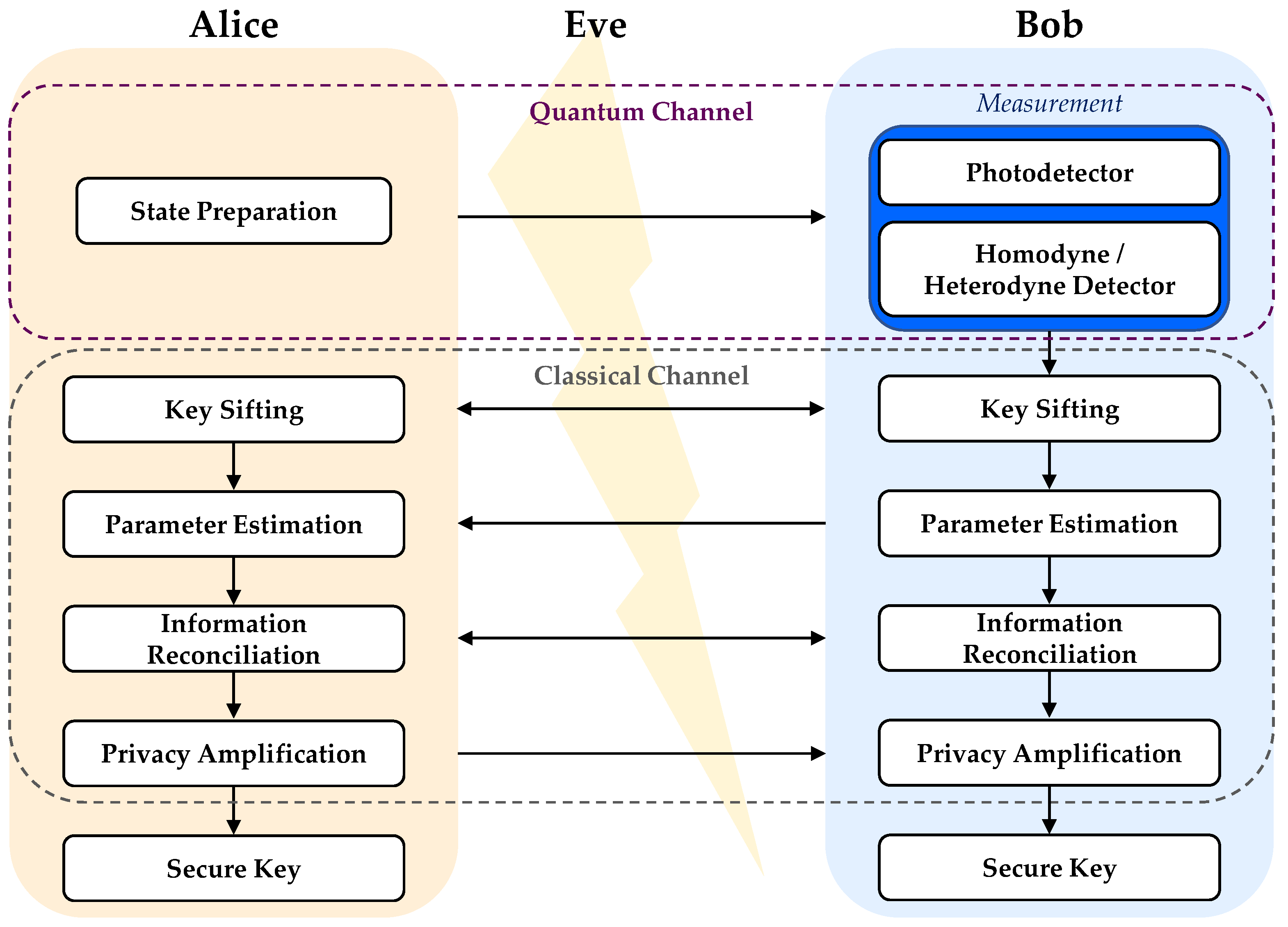
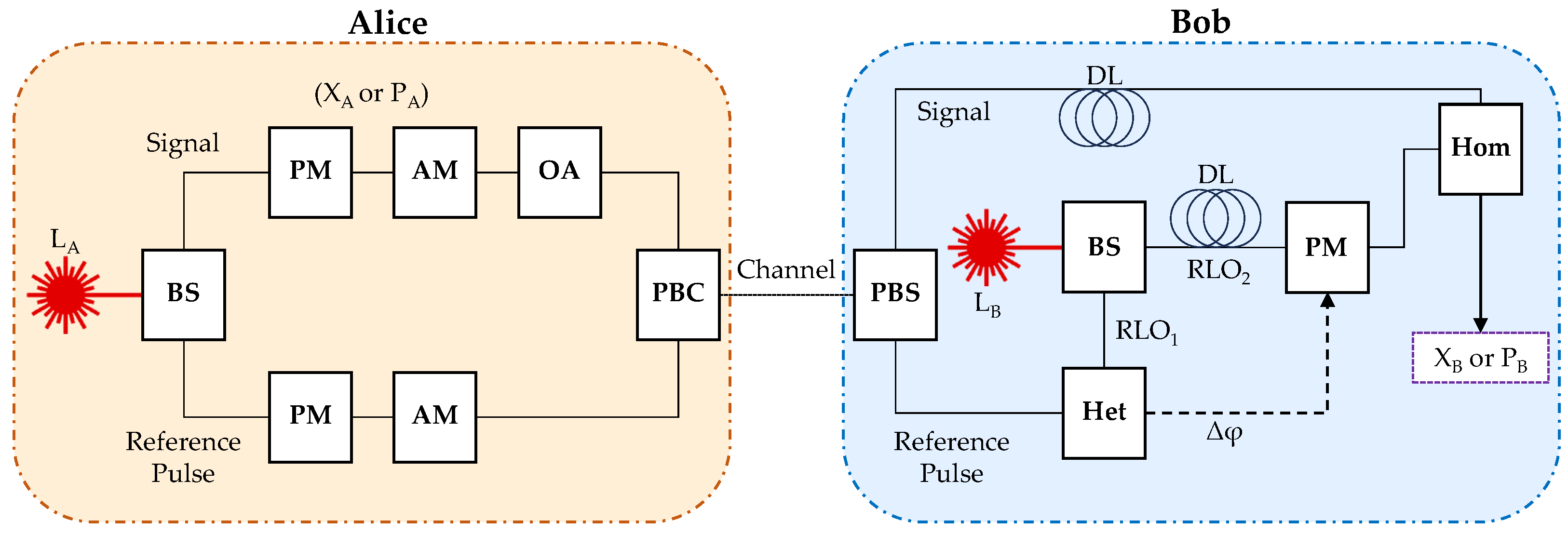
2. CV-QKD Overview

CV-QKD involves two legitimate parties: Alice (represented by subscript A), who prepares quantum signals at a transmitter, and Bob (represented by subscript B), who measures the signals at a receiver. A third party, Eve, is considered malicious with the objective to eavesdrop on the quantum channel and/or detector.

In the CV domain, quantum information is usually encoded on the electric field quadratures of light, where the quadrature values X and P represent the in-phase and out-of-phase components of the electric field. The coherent state, which can be labeled $|\alpha \rangle =|X+iP\rangle$, is usually adopted for the encoding. This state is defined as [48],

$$|\alpha \rangle =e^{-\frac{1}{2}{\left|\alpha \right|}^2}\sum _{n=0}^{\infty }\frac{{\alpha }^n}{\sqrt{n!}}|n\rangle ,$$

(1)

in the basis of Fock states $|n\rangle$, where $\alpha$ is the amplitude and n is the photon number. The encoded quantum signal (henceforth referred to simply as the signal) can be measured using homodyne or heterodyne detection at the receiver. Homodyne detection involves measurement of either the X or P quadrature, while heterodyne detection involves measuring both the X and P quadratures simultaneously. In what is to follow, unless otherwise stated, we will assume homodyne detection is used. The consideration of heterodyne measurements follows a similar path to what is given, with the simultaneous measurement of both quadratures incurring an additional noise penalty [49]. Figure 1a illustrates the so-called phase-space diagram for encoding in coherent states, where we have defined the angle $\theta$ and amplitude $\alpha$ of the states as $\theta =arctan(P/X)$ and $\alpha ={(X^2+P^2)}^{1/2}$. We caution that the development of a “phase operator” in quantum optics has a somewhat complex history, and care must be used in interpreting the angle $\theta$ in regard to the classical phase $\varphi$ of the electromagnetic wave. A phase operator can be developed that shows that $\theta \to \varphi$ in the large photon limit (classical limit). When we later discuss the use of phase measurements on reference pulses, we can consider that we are measuring $\varphi$ on those pulses, with $\varphi =0$ being defined as the reference pulse phase at the transmitter. For a more detailed description of coherent states, the phase-space representation of quantum states, the development of a phase operator, and the relationship between $\theta$ and $\varphi$, the reader is referred to [48].

CV-QKD protocols can, to a large extent, be separated into two main categories, GMCS CV-QKD and DM CV-QKD. GMCS CV-QKD involves randomly selecting quadrature values from independent Gaussian distributions with modulation variance $V_{mod}$, $X,P\in \mathcal{N}(0,V_{mod})$, which can be seen in Figure 1a, where the Gaussian distribution for X is shown in red and the Gaussian distribution for P is shown in blue. Unlike GMCS CV-QKD, DM CV-QKD involves encoding discrete values of the quadratures onto the signals. Encoding is usually achieved by modulating the quadratures through phase-shift keying (PSK) or quadrature amplitude modulation (QAM). In such encoding, a trade-off between increased information transfer and increased difficulty in measuring a larger pool of discretized states will be in effect. As example cases, two of the most common PSK protocols are the four-state quadrature PSK protocol, given in Figure 1b, and the eight-state 8PSK protocol, given in Figure 1c. It is important to note that GMCS CV-QKD security proofs are more mature than those of DM CV-QKD [50,51]. However, DM CV-QKD has shown higher reconciliation efficiencies than GMCS CV-QKD at longer distances [52,53] and at lower signal-to-noise ratios (SNRs) [54].

A generic CV-QKD protocol, which applies equally to GMCS and DM CV-QKD, involves the following steps:

1.

Alice prepares and transmits states $|\alpha \rangle =|X_A+i{P}_A\rangle$ encoded on the signal across a channel (e.g., optical fiber or FSO).

2.

Bob measures $X_B$ or $P_B$ of the signal using his homodyne detector.

3.

Key sifting is performed, whereby Alice and Bob decide which variables are to be used for key generation, discarding any uncorrelated measurements.

4.

Parameter estimation is undertaken to analyze the system parameters (transmissivity and excess noise), from the amount of mutual information shared by Alice and Bob can be determined, as well as how much information Eve has access to.

5.

Information reconciliation is carried out, in which, after the digitization of the symbols (using some pre-assigned scheme), an error correction code is used to correct differences in the keys held by Alice and Bob.

6.

A confirmation protocol (usually via the use of hash functions) is used to bound the probability that the error correction has failed.

7.

Finally, privacy amplification is performed on the keys, shortening their length, to reduce Eve’s information on the key to a pre-assigned negligible level (again, usually via hash functions).

An overview of the generic CV-QKD protocol is given in Figure 2, where the current works on ML assistance for CV-QKD are highlighted at each step of the protocol.

Note in the above, a pre-shared secret key is used to authenticate all necessary classical communications. The presence of such an a priori shared key is why QKD is perhaps better described as a quantum key growing process. We also note that, for the purpose of the homodyne measurements for Bob, a transmitted local oscillator (TLO) is usually multiplexed with the signal for coherent measurement at the receiver. However, TLOs can be attacked and manipulated by Eve [56]. This has led to the use of real local oscillators (RLOs), also known as local local oscillators, which are phase-corrected using reference pulse information multiplexed with the signals. This latter approach using RLOs can be considered state-of-the-art for CV-QKD [57,58]. We have not attempted to provide a complete methodology of CV-QKD here. A more in-depth explanation of relevant CV-QKD protocols and procedures can be found in the recent survey on CV-QKD [59], while the practical implementation of GMCS CV-QKD is outlined in [49], and a security analysis of DM CV-QKD is given in [51].

Figure 3 illustrates a specific schematic of the preparation, transmission, and measurement of coherent states, including phase compensation using an RLO-based scheme, described as follows. At Alice, a laser source, $L_A$, is passed through a beam splitter to generate the light source (coherent states) for the signals and reference pulses. The (quantum) signals are encoded with randomly selected quadrature values, $X_A$ or $P_A$, while the much stronger (classical) reference pulses are encoded with pre-assigned quadrature values (known publicly). The signals and reference pulses are then polarization multiplexed using a beam combiner and transmitted across the channel to Bob, who de-multiplexes them. A laser source, $L_B$, at the receiver is split into two RLOs: RLO${}_1$ and RLO${}_2$. The first of these, RLO${}_1$, is used to measure the reference pulses via heterodyne detection. These quadrature measurements allow us a first estimate of the phase error $\Delta \varphi$, the phase difference between the transmitted and received reference pulse [58,60,61,62]. This $\Delta \varphi$ is then used to phase-correct the second RLO, RLO${}_2$. Then, by combining the signal and the phase-corrected RLO${}_2$ in a homodyne detector, one of the signal’s quadratures, $X_B$ or $P_B$, is measured (the signal and RLO${}_2$ are delayed in this scheme). Note, in the literature this method of phase-adjustment to the RLO${}_2$ if often termed “phase compensation”.

The phase compensation technique described above represents but one type of implementation; however, it is important to realize that in essence all implementations have the same aim: the determination of the signal’s quadratures corrected for errors incurred in the preparation, transmission, and measurement of the signal. In the context of CV-QKD, these errors in the signal’s quadratures translate into excess noise [49], a noise beyond vacuum fluctuations that impact key rates negatively [49].

However, the measured $\Delta \varphi$ does not exactly predict the phase error between the signal and RLO${}_1$—a remnant phase error, $\Delta {\varphi }^{\prime }$, between the signal and the RLO${}_2$ exists. This remnant phase error is due to several real-world limitations of the phase compensation method outlined above. Firstly, both the signals and reference pulses possess 2-dimensional phase wavefronts, where distortion of the wavefronts is not uniformly distributed. The resulting $\Delta \varphi$ value is obtained after integrating across the reference pulse wavefront ${\mathsf{\Phi }}_{rp}(x,y)$. As such, the phase-correction of the RLO${}_2$ wavefront ${\mathsf{\Phi }}_{RL{O}_2}(x,y)$ using $\Delta \varphi$ leads to inconsistencies across the wavefronts: ${\mathsf{\Phi }}_{RL{O}_2}(x,y)\ne {\mathsf{\Phi }}_{rp}(x,y)$, which contributes to $\Delta {\varphi }^{\prime }$ [58,62]. Other contributions to $\Delta {\varphi }^{\prime }$ are introduced by the independent laser sources $L_A$ and $L_B$, through such factors as inaccurate clock synchronization and unequal spectral linewidths of the lasers [60,61]. Furthermore, the signals and reference pulses can interact differently with the channel due to their different polarizations, adding to $\Delta {\varphi }^{\prime }$, as can contributions associated with the signal and RLO${}_2$ propagating through delay lines [60,61].

In the context of this review, we note that ML has been used for $\Delta {\varphi }^{\prime }$ reduction at different stages of the signal quadrature measurement process, including being embedded in the system such that the $\Delta {\varphi }^{\prime }$ estimate is incorporated into the phase-correction of the RLO [13], the correction of the measured signal quadratures in post-processing using the estimated $\Delta {\varphi }^{\prime }$ [5,6,15], and the application of an estimated correction to the wavefront of the RLO [16]. Moreover, ML offers potential improvements in computational efficiency for key sifting, reconciliation, and key rate estimation procedures, improving the feasibility of real-time CV-QKD. Next, we discuss the relevant ML algorithms in detail.

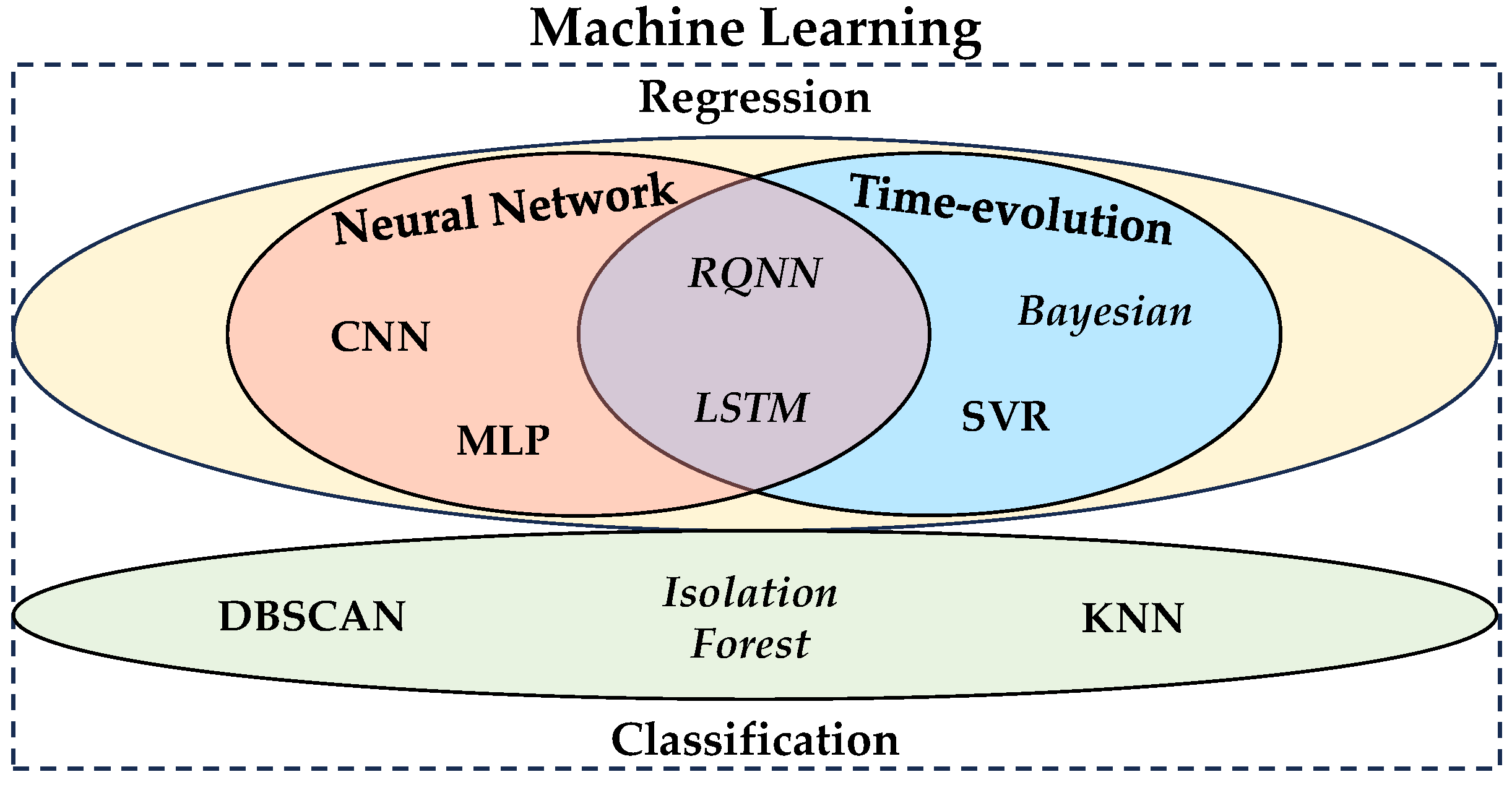
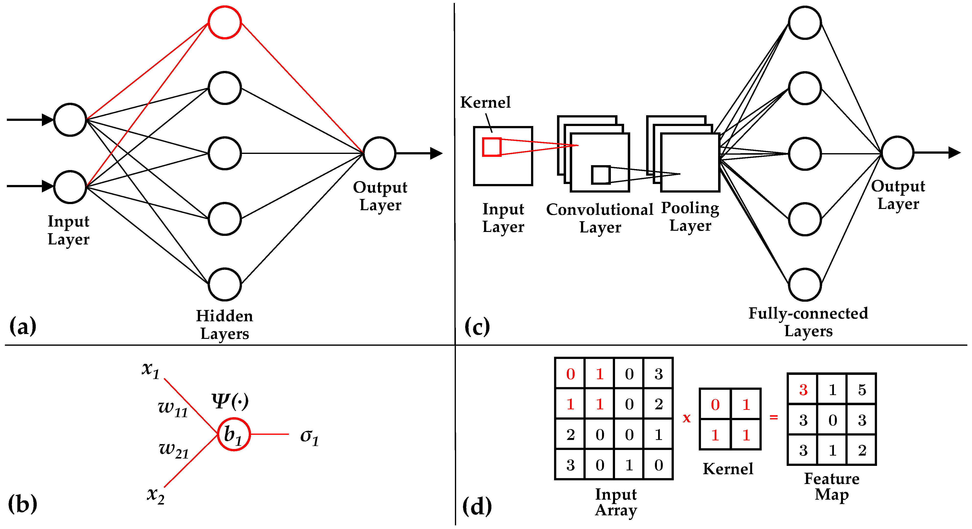
3. Machine Learning Methods

ML is a subclass of artificial intelligence, where we define ML as an algorithm designed to learn patterns from a data set, without being specifically programmed with a set of rules on how to do so.

ML encompasses a very wide variety of algorithms types, which have been be categorized in several ways, sometimes with fuzzy distinctions between categories. This work does not present an in-depth review of ML methodologies; we would recommend [63] for a recent survey on ML algorithms, their applications, and their future directions. Instead, we outline some key distinctions between ML algorithm types and then briefly introduce some example algorithms to give readers with limited ML experience some perspective on the works presented in Section 4, Section 5, Section 6 and Section 7.

The first distinction between ML algorithms is that they can either be supervised or unsupervised when learning from data. In supervised ML, data are split into training and testing data sets, whereby a model is constructed to map the relationship between known inputs and known outputs using the training data. The test data are then used as input to the trained model to test their output estimation performance. Unsupervised ML models are designed to analyze unlabeled data, discovering patterns in the data without being given example outputs, generally to cluster data, form associations, or to perform dimensionality reduction.

Secondly, the output of a ML algorithm can either be continuous, forming regression algorithms, or discrete, forming classification algorithms. Further, both regression and classification ML algorithms can either incorporate the time evolution of a system or not when constructing relationships from the data, representing another distinction between ML algorithm types.

Neural networks (NNs) are a popular subclass of ML, themselves encompassing a wide range of algorithm types, which can be used for supervised or unsupervised learning, classification, regression, and time-series analyses. At their core, NNs are comprised of a series of layers, where weighted connections are formed between features in consecutive layers. Data are fed into an input layer, then a relationship is mapped to an output layer via one or more hidden layers. Deep learning is a subclass of NN, where the depth of the NN represents the number of hidden layers within it. The consensus on the exact number of hidden layers required for an algorithm to be considered deep is fuzzy, though we will define any NN with more than three hidden layers as a deep learning algorithm.

Figure 4 outlines a taxonomy of the ML algorithms included in this survey on ML-assisted CV-QKD. As can be seen, all of the algorithm types fall under the title of ML, with regression and classification algorithms forming two distinct categories. The distinction between supervised and unsupervised ML algorithms is identified by the unsupervised algorithms written in italics (with supervised algorithms written in normal text). As mentioned, while NN and time-evolution algorithms are only presented within the regression category, their disconnect from classification applies only to the work contained within this survey. NNs can be used for both classification and time-evolution analyses.

A multi-layer perceptron (MLP) is a simple feedforward NN, which takes a vector as input. Perceptrons (nodes) in each layer of the MLP receive inputs $x_i$ from the perceptrons i in the previous layer, manipulating the input data using an activation function $\psi (·)$ to calculate the output of each perceptron ${\sigma }_j$ as,

$${\sigma }_j=\psi (\sum _{i=1}^n{x}_i{w}_{ij}+b_j),$$

(2)

using the weight $w_{ij}$ on the $ij$-th path, and a bias term $b_j$ of the relative importance of the activation function. Backpropagation then passes error information back through the layers to update the network weights and biases during training. The error is calculated layer-by-layer, where a type of optimization (often gradient descent) is used to minimize a cost function (often mean squared error), improving the estimation results. Different types of activation functions are used for different purposes. For example, the rectified linear unit function is one of the most commonly used activation functions for hidden layers, where $\psi \left(x\right)=0$ if $x<0$, else $\psi \left(x\right)=x$ if $x\ge 0$. A linear activation function is commonly used in the output layer of NNs designed for regression, such that the output can take any continuous value, while sigmoid activation functions are commonly used for classification NNs to return discrete outputs. In the surveyed works, MLPs were applied to excess noise filtering in [12], parameter optimization in [26], reconciliation in [29], and key rate estimation in [30].

Figure 5a gives an example of a generic fully connected MLP, where the connections between the input layer, hidden layer, and output layer are shown, as well as an example perceptron in Figure 5b, indicating how the inputs and weights from the previous layer are transferred into an output via the activation function (following the path outlined in red).

Convolutional neural networks (CNNs) are another common architecture type of NN, which take an n-dimensional array as input (usually two- or three-dimensional), such that spatial relationships between array elements are exploited. CNNs are generally constructed using three layer types: convolutional layers, pooling layers, and fully connected layers. In convolutional layers, a kernal (filter) is passed over a sub-array of the input data, sifting out a feature map of the relationships between elements. The pooling layers then decrease the size of the convolved feature map to reduce the network’s computational complexity. Often, pooling layers are flattened into a vector to use as input for fully connected layers, which construct the model output. Fully connected layers are the same as hidden layers in an MLP, where each perceptron in each layer is connected to every perceptron in the next. Figure 5c gives an example of CNN architecture, outlining common layer types and the mapping of a two-dimensional array as input to a vector output. Figure 5d then gives an example convolution of an input array to a feature map. Surveyed works include CNNs developed for wavefront correction in [16] and $\Delta {\varphi }^{\prime }$ reduction in [13].

Note that the subsequent survey of literature on ML assistance for CV-QKD includes works using Bayesian inference methods combined with a type of Kalman filter (KF), defined as ML in [5,6,7,8,9,10,11], as well as combined with particle smoothing, defined as ML in [17,18,19], though it does not include literature where Bayesian inference alone has assisted CV-QKD (as in [64]).

3.1. Regression

Encoder–decoder NNs are a type of supervised NN commonly used for regression. The encoder maps relationships from input data points to a reduced feature space; then, the decoder uses the reduced feature space to reconstruct a prediction of the output space. For example, image-to-image translation can be undertaken using encoder–decoder NNs, such as transforming a picture from a summer scene to a winter scene. Using the example, the common structure between an image in summer and winter would be encoded into the reduced feature space, while the adaptation to winter would be constructed in the decoder. CNNs are often used as encoder–decoder NNs, for which the architecture in Figure 5c could be used as the encoder; then, an inverse architecture could be used as the decoder. Note that encoder–decoder NNs can also be used for classification. Surveyed works used encoder–decoder NNs for wavefront correction [16] and excess noise reduction [14].

3.2. Classification

One of the most common supervised ML classification algorithms is the k-nearest neighbor (KNN) algorithm. Test data points are connected to their k-nearest matching neighbors from the labelled training data by measuring their distances, then classified as being in the group containing the most neighbors. Distance-weighted KNN algorithms extend the original KNN methodology by including a weighting to each of the k-nearest neighbors, such that closer neighbors are prioritized. The value of k should be tuned to minimize misclassification. Turbulence strength classification using a KNN algorithm was undertaken in [12], while DM CV-QKD state classification using KNN algorithms was undertaken by [21,22,24]. Note that no works on ML-assisted CV-QKD utilized an NN for classification.

3.3. Time Evolution

Recurrent NNs represent a subclass of NN designed to store time-series data in a form of memory, such that dependencies can be mapped between the previous data inputs and the next output instance in the series. Essentially, a feedback loop is created, where the network weights and biases of previous time instances are fed into the activation function of the consecutive time instance, forming recurrent layers. A long short-term memory (LSTM) NN is a type of recurrent NN that incorporates a memory cell, which controls the information fed back into the network at consecutive time instances, retaining or discarding certain information to form long-term dependencies. While LSTMs are considered as unsupervised NNs, they have been described as self-supervised given that they learn relationships from the error of previous time instances, and they can be designed for both regression and classification. The surveyed works [14,20] used an LSTM and a type of recurrent NN for excess noise filtering, respectively, while [15] used an LSTM for $\Delta {\varphi }^{\prime }$ reduction.

3.4. Unsupervised Learning

Isolation forest algorithms are a type of unsupervised learning ML algorithm used for anomaly detection (a type of classification). Isolation forest algorithms work by forming isolated trees, where the tree randomly selects a dimension from a data set and then randomly splits the data along that dimension. Each of the new subspaces form their own sub tree. This process is repeated until every data point has been isolated as its own leaf node; then, the whole process is repeated for multiple isolated trees, which form a forest. The algorithm traverses each tree, assigning a score to each leaf as a function of its depth in the tree, where it is assumed that anomalous data will be isolated along a shorter path length. The data point with the lowest composite score across all trees in the forest is output as the anomalous data point. The removal of abnormal data points for key sifting using an isolation forest algorithm was undertaken by [28].

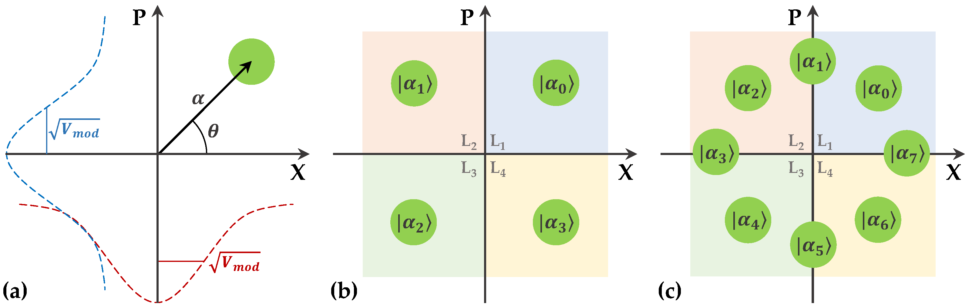
4. Gaussian Modulated Coherent State CV-QKD

The primary application of ML for GMCS CV-QKD has been recovering the transmitted quadrature measurements X or P at the receiver. This has been achieved using four different approaches. The first was $\Delta {\varphi }^{\prime }$ reduction, where an estimated $\Delta {\varphi }^{\prime }$ was obtained from the reference pulses and then used to phase-correct the RLO for the coherent measurement of the signal [13]. The second was the correction of the signal quadratures in post-processing using $\Delta {\varphi }^{\prime }$ estimates [5,6,15]. The third was, more broadly, the excess noise filtering of the signal quadratures in post-processing [12,14], not focusing specifically on the phase noise. The fourth was correction of the RLO wavefront using reference pulse wavefront estimations [16]. Note that these approaches to signal recovery for GMCS CV-QKD used regression-type ML algorithms.

A Bayesian inference-unscented KF $\Delta {\varphi }^{\prime }$ reduction technique was developed in [5]. A state space model of reference pulse evolution over time was implemented according to discrete Markovian dynamics, with an included the $\Delta {\varphi }^{\prime }$ term. The Bayesian inference-unscented KF model was used to evaluate a probability distribution of $\Delta \varphi$ at each time step, using the current and previous reference pulse heterodyne measurements and $\Delta \varphi$ estimations, such that the distribution represented the $\Delta {\varphi }^{\prime }$ distribution, and the mean represented the optimal estimation of $\Delta \varphi$. This process allowed the algorithm to update itself based on information from the reference pulses in real-time. The Bayesian inference-unscented KF method was compared to a standard reference method and an extended KF, where it was found to outperform both of them in terms of excess noise filtering (by reducing the phase noise term), particularly for low SNRs, which resulted in higher key rates. An extension of [5] was published in the work [6], where a joint polarization and $\Delta {\varphi }^{\prime }$ reduction model was developed based on the same Bayesian inference-unscented KF approach. Higher key rates were achieved using the proposed ML algorithm than a presented traditional constant modulus algorithm. The phase correction methodology of [5] was then applied to several works, including [7] for their work on CV-QKD across a 60km optical fiber channel, then again across a 100km optical fiber channel [8], as well as in another work on modulation leakage-free CV-QKD [9]. Further, the authors of [10] implemented the same methodology in their research on a practical CV-QKD approach with composable keys and again in another work on modulator vulnerabilities in CV-QKD [11].

Another approach to $\Delta {\varphi }^{\prime }$ reduction was developed in [13] using a CNN architecture. The input to the CNN was discussed as being the reference pulse quadratures, defined by an array of dimension 5 × 2, while the output was an estimate of $\Delta \varphi$ to apply to an RLO, incorporating $\Delta {\varphi }^{\prime }$. Figure 6 gives a schematic of the measurement methodology of [13], showing how the CNN was incorporated into the measurement process. Of note, the authors incorporated the frequency offsets and phase jitter of $L_A$ and $L_B$ into their model of $\Delta {\varphi }^{\prime }$. The results from the CNN were compared with those attained using a KF, showing that the CNN estimated $\Delta {\varphi }^{\prime }$ more accurately than the KF across a range of SNRs.

In order to compensate for signal distortion across an optical fiber channel, the authors of [15] developed an LSTM NN to learn the long-term dependencies of $\Delta {\varphi }^{\prime }$ over time, predicting $\Delta {\theta }^{\prime }$ at current and future time steps. Unlike previous approaches, a TLO was used, where Bob measures the signal quadratures and then trains the NN using the quadrature measurements and historic $\Delta {\theta }^{\prime }$ information. The $\Delta {\theta }^{\prime }$ estimations were then sent to Alice such that she could reconstruct her quadrature values. It was stated that the advantage of their proposed signal recovery methodology was maintaining the security of the CV-QKD system without requiring additional hardware or quantum resources. Key rates were calculated for the case of perfect $\Delta {\theta }^{\prime }$ estimation, no $\Delta {\theta }^{\prime }$ estimation, and using the LSTM $\Delta {\theta }^{\prime }$ estimation method, where results showed the LSTM-based case approached the perfect $\Delta {\theta }^{\prime }$ estimation case across a range of channel lengths, while the case of no $\Delta {\theta }^{\prime }$ estimation performed significantly worse.

A noise filtering methodology was developed in [14] using an LSTM and autoencoder to estimate corrected quadrature measurements, where the primary emphasis was on noise introduced by the nonlinear imperfections of the balanced homodyne detector and consequent analogue-to-digital converter (termed inter-symbol interference reduction). When received signal pulses repetition rates were lower than the homodyne detector’s, the amplitude of the signal was maintained; however, as repetition rates increased, the lag of sequential signal pulses overlapped. Further, as the sampling frequency of the analogue-to-digital converter should match that of the signal pulse duration, the mismatch of the system bandwidth and sampling frequency led to nonlinear distortions of the quadrature measurements. Increased repetition rates greatly improved the secure key bit rate. The autoencoder was used as a noise filtering NN, where its encoder and decoder architectures were constructed using LSTM layers, such that the LSTM memory component could be used to harness the time-based relationships between signal pulses. The NN was trained on three different signal pulse repetition rates: 250 MHz, 500 MHz, and 1 GHz. While positive key rates were possible without the noise filtering algorithm for the 250 MHz case, the 500 MHz and 1 GHz cases resulted in null key rates. However, once the noise filtering NN algorithm was applied, excess noise was reduced below the null key rate threshold. The results indicated how ML can assist in increasing the secure key bit rate across a channel by compensating for noise introduced by CV-QKD hardware.

An equalization method, assisted by an MLP, was developed in [12] to reduce excess noise in the signal quadrature measurements across an optical fiber channel. The authors then applied their equalization methodology for an FSO channel, such that a KNN algorithm was used to classify turbulence strength; then, a different equalization MLP was trained for each turbulence class, where each NN had a different set of connection weights and perceptron biases. The results showed that signal quadrature measurement corrections were improved when the classification scheme was implemented, particularly for channels with medium-to-strong turbulence.

An alternative approach to phase error reduction after signal distortion across a satellite-to-ground channel was undertaken in [16]. An encoder–decoder CNN architecture was used to estimate wavefront corrections to apply to an RLO, using only the reference pulse spatial intensity distributions as input to the CNN, in order to achieve the coherent measurement of signals. The results showed the estimated corrections were able to increase the coherent efficiencies of the measurements for varying satellite altitudes and turbulence strengths, resulting in non-zero key rates and removing the need to measure the wavefront directly.

Phase compensation can be undertaken during the measurement process using digital signal processing and RLO modulation [13,16], or using digital signal processing alone [5,6,15]. The use of hardware to modulate the RLO requires additional time for actuation, which can introduce its own errors but leads to the measurement of signals with greater coherence. Digital signal processing can be applied in post-processing, where noise sources beyond phase error can be filtered and the time required for hardware actuation in-the-loop is removed. Thus, using digital signal processing alone could increase the real-time feasibility of a CV-QKD system. However, we note that the errors in the measurement will be greater, and this could lead to less accurate phase compensation overall. When modulating the RLO, channel conditions should be taken into consideration when determining how to measure reference pulses for phase compensation. Signals that pass through atmospheric turbulence and experience uneven phase distortion across their wavefront should use a wavefront sensor to measure the reference pulses (as in [16]), such that the RLO wavefront can be heterogeneously modulated. However, if the assumption of even-phase errors across the signal wavefront is applicable, then heterodyne detection can be used to measure the reference pulses. The aforementioned assumption is likely applicable to FSO channels with weak turbulence.

5. Discretely Modulated CV-QKD

Similarly to GMCS CV-QKD, ML algorithms designed for excess noise filtering [20] and $\Delta {\varphi }^{\prime }$ reduction [17] have been applied to DM CV-QKD, where the recovered signal was then classified as one of the discrete states used in the DM protocol (i.e., PSK or QAM states). However, unlike GMCS CV-QKD, classification ML algorithms have also been applied to state discrimination in DM CV-QKD, such that the output of the algorithms is the discrete state classification itself [21,22,24], as well as modulation format identification [23].

A distance-weighted KNN was used to classify states measured by Bob for a four-state quadrature PSK DM CV-QKD protocol (as shown in Figure 1b) in the work [21]. Errors rates were compared against SNRs for the distance-weighted KNN approach and a traditional maximum likelihood classification scheme, where the KNN classification resulted in lower error rates (misclassifications) across the entire SNR range, with greater improvements at higher SNRs. Secure key rates were also calculated for varying channel lengths and modulation variances, with the ML-assisted classification model outperforming the traditional approach in each case. The improvement in secure key rates using the distance-weighted KNN was more pronounced for longer channels and greater modulation variance values.

A multi-label classification algorithm, based on KNN, was developed in [22] to classify 8PSK states. Each quadrant was given a label $L_i(i=1,2,3,4)$, where each discrete state uses a single label in quadrant PSK, as depicted in Figure 1b. However, for 8PSK, states $|{\alpha }_1\rangle$, $|{\alpha }_3\rangle$, $|{\alpha }_5\rangle$, and $|{\alpha }_7\rangle$ simultaneously belong to two labels each, as shown in Figure 1c. A feature vector of Euclidean distances to each of the 8PSK state quadrature locations was constructed for each received state to use as input to the classification algorithm. KNN was performed, and then posteriori probabilities were calculated for the condition of the received state belonging to a label, applying the label when a threshold probability was reached. The key rates calculated for a range of channel lengths and modulation variances were compared for the proposed 8PSK classification algorithm, as well as quadrature PSK, 8PSK, and GMCS CV-QKD, all without the classification algorithm. It was found that the proposed approach achieved higher key rates than each of the protocols without the classification algorithm, except for across short channels (approximately <10 km).

A quantum KNN algorithm was designed for state classification for 8PSK DM CV-QKD in [24]. This quantum KNN algorithm differs from a classical KNN by using quantum computation to simultaneously calculate the distances between an unclassified state and its KNNs. The algorithm then sorts the distances using an optimization technique based on the Grover’s algorithm to find the closest neighbors. The authors outline a theoretical security proof of this specific quantum KNN algorithm using a semi-definite program method, where they show that less Holevo information was accessible to Eve than to a classical KNN algorithm. Secure key rates were compared for traditional quadrature PSK, 8PSK, and the proposed quantum KNN algorithm, with the quantum KNN algorithm having higher key rates across a range of modulation variances and channel-noise conditions. In [24], key rates were not calculated for a classical KNN algorithm applied to state classification in DM CV-QKD, though a complexity analysis demonstrated the increased computational efficiency attained by the quantum KNN algorithm when compared to a classical KNN. The work of [24] provides an in-depth definition of their methodology; however, it should be noted that the work is purely theoretical as quantum computation has not reached the level of maturity required to execute the algorithms.

One work [17] investigated a DM CV-QKD protocol without sending an RP or TLO, only using an RLO and a noise filtering particle smoother model based on Bayesian inference, which filtered the signal quadrature measurements for $\Delta \theta +\Delta {\theta }^{\prime }$ reduction. The Bayesian particle smoother was trained using a Monte Carlo Markov chain method, which optimized the tracking of dynamic signal distortion using the set of keys shared between Alice and Bob for parameter estimation. Experimental and simulated data were used to test their noise filtering methodology for both binary PSK and quadrature PSK, with the cases of 0%, 5%, and 100% of the keys being used to train the Bayesian model. Using simulated data, excess noise was reduced by approximately an order of magnitude at low SNRs when $100\%$ of keys were shared, compared to $5\%$, before converging on similar noise levels at higher SNRs. The results were volatile for $0\%$ shared measurements at low SNRs. The experimental results showed that for low SNRs, the cases of 5% and 100% of shared measurements had similar noise filtering efficiencies, both improving upon the 0% case. The absence of a TLO or RPs in the protocol presented in [17] could help to mitigate security vulnerabilities introduced by their transmission, as well as reduce system complexity. Two works that used the same methodology were also published [18,19].

While [17,18,19,21,22] applied ML to aid in state discrimination for fixed PSK state modulation schemes, the authors of [23] investigated a variable modulation scheme for increased network adaptability and receiver flexibility. A density-based spatial clustering of applications with the noise (DBSCAN) algorithm was implemented for modulation format identification, which could identify M-QAM protocols, assuming that Alice had not informed Bob of which modulation scheme was being used. DBSCAN classified the received states as being modulated using a 4-QAM, 16-QAM, 64-QAM, or 256-QAM scheme, where it was shown that higher M-QAM values resulted in higher key rates across a range of channel lengths. When comparing SNRs with the success rates of correct modulation format identification, lower M-QAM values could achieve higher success rates at lower SNRs. For example, 100% success rates were attained for 4-QAM at an SNR of ∼10 dB, while 256-QAM required an SNR of ∼23 dB. The accuracy of DBSCAN was found to increase as the number of training samples increased. One advantage of DBSCAN over other clustering techniques (such as KNN) is that the number of clusters was determined by the algorithm itself rather than being defined by the user.

Lu et al. [20] implemented a recurrent quantum NN (RQNN) to assist in coherent state $\psi (x,t)$ recovery for a two-state coherent polarization CV-QKD protocol, where the input to the RQNN was the signal quadrature measurements and the output was the filtered signal. It was assumed that the probability density function (PDF) of the Schrödinger equation, calculated as,

$$i\hslash \frac{\partial \psi (x,t)}{\partial t}=-\frac{{\hslash }^2}{2m}{\nabla }^2\psi (x,t)+V(x,t)\psi (x,t),$$

(3)

could act as a stochastic filter of noisy signals, where ℏ is the Planck constant, m is mass, and ($x,t$) represent the spatial and temporal coordinates of the quantum state. The spatial potential $V(x,t)$ of the Schrödinger equation, given by,

$$V_j(x,t)={\varphi }_j\left(\nu \left(t\right)\right)\left(\sum _{i=1}^n{w}_{ij}(x,t)\right),$$

(4)

was implemented as the activation function of each perceptron. The recurrent input of the RQNN was an expected error term $\nu \left(t\right)$, which was used to construct $V(x,t)$ via a Gaussian kernel function $\varphi \left(\nu \right(t\left)\right)$, where the connection weights between perceptrons were modified to update $V_j(x,t)$ for each perceptron j. The summed $V(x,t)$ from the output of the perceptrons in the second layer was used to update the Schrödinger equation, which was then used to calculate the PDF as ${\left|\psi (x,t)\right|}^2$. Noise parameters were calibrated at each time step for each noise source, constructing $\varphi \left(\nu \right(t\left)\right)$, which was stated as the core process of the RQNN. By adjusting the PDF, the RQNN decreases the expectation error, improving the accuracy of the filtered signal. The noise filtering performance of the RQNN was compared with a KF and an MLP. Similar noise filtering performance was found for all approaches, given unlimited computational time; however, the RQNN was able to achieve the same performance in far less time. Further, when compared with the MLP, the RQNN is an unsupervised ML algorithm and thus does not need to be trained on existing data beforehand and is able to adapt to unknown fluctuations in the channel. The ML classification of coherent polarization states has not been investigated, while more research should be undertaken to understand the advantages and disadvantages of encoding information using the polarization of coherent states, when compared to quadrature encoding.

6. Parameter Estimation and Optimization

Beyond the signal recovery and state discrimination methods given in Section 4 and Section 5, effective parameter estimation and optimization can further improve secure key rates for CV-QKD, where ML has been used to assist in predicting the time evolution of intensity distributions [25], modulation optimization [26], and key estimation for parameter estimation [55].

A support vector regression (SVR) model was adopted in [25] to predict the time evolution of the intensity of the laser source at the transmitter and TLO at the receiver in their CV-QKD setup. Experimental intensity distributions were used to train and test the SVR model, with a radial basis function kernel used to fit the hyperparameters of the predictive function. The distorted TLO intensity predictions were then used to amplify or attenuate the TLO at the receiver to compensate for the predicted intensity fluctuations. Secure key rates were analyzed across a range of channel lengths for the proposed SVR-based dynamic TLO intensity modulation approach and a traditional stabilization technique. The SVR-based approach achieved higher key rates across all channel lengths, as well as increasing the maximum channel length where non-zero key rates are attained (up to approximately 50 km, compared to 45 km using the traditional method). The fluctuations in TLO intensity can be exploited by Eve to conceal attacks on the system, highlighting the need for accurate TLO intensity predictions to identify whether signal distortions are channel or hardware-based versus introduced by Eve.

A signal modulation technique in [26] utilized an MLP to optimize modulation variance for a DM CV-QKD protocol as a function of FSO channel conditions. Specifically, the Rytov variance (as a function of refractive index structure parameter $C_n^2$), transmissivity, and channel length were used as input to an MLP to map a relationship to the optimal modulation variance output for the varying channels, as outlined in Figure 7. A horizontal FSO channel (fixed $C_n^2$) was simulated, of length 0 to 11 km, with beam wandering, broadening, and deformation all accounted for in the calculation of transmissivity. Higher key rates were achieved when the MLP-based signal modulation optimization was applied, compared to a traditional local search algorithm, though it was not stated which local search algorithm was tested.

The work [55] used an MLP to estimate Alice’s key string by mapping the relationship between a proportion of Alice and Bob’s normalized keys during training, then using the trained MLP to estimate the rest of the key. The objective was to use the estimated key for parameter estimation. Their results indicated that higher key rates could be achieved using their methodology than a claimed conventional scheme.

While [55] used ML for parameter estimation for CV-QKD, no works have investigated the use of ML for parameter estimation for FSO channels, where turbulence can lead to greater fluctuations of the channel parameters. ML could be better suited to channel characterization when channel conditions are highly volatile. Further, a combined approach to signal intensity and variance modulation could lead to improved key rates, rather than single variable optimizations (as in [25,26]).

7. Key Sifting, Reconciliation, and Key Rate Estimation

ML algorithms have also been applied to key sifting [28], information reconciliation [29], and key rate estimation [30,31], with [29,30,31] providing examples of improved computational efficiency of NNs over traditional approaches, while [28] gives an example of ML used for anomaly detection.

One method for key sifting in [28] used an isolation forest ML algorithm to sift out abnormal bits, affected by noise, from the raw key. After uncorrelated keys were discarded, the remaining bits were divided into equal-sized miniblocks to input to the isolation forest algorithm, which recursively split the data until each bit was isolated. An anomaly score was calculated as a function of each bit’s height in the miniblock tree to calculate the probability of them being anomalous. Anomalies were introduced to 0.3% of miniblocks of size ${10}^3$ bits, where noise was introduced to 20% of the anomalous miniblocks. Excess noise filtering was compared between the isolation forest method and a traditional Wiener filter for anomalous bit detection, where noise filtering was found to be similar for both methods across a range of channel distances up to 100 km. Key rates showed a similar trend, though the Wiener filter approach resulted in slightly higher key rates for most channel conditions. This work presented an example of a traditional algorithm outperforming ML in terms of anomaly detection, highlighting the need to not blindly apply ML algorithms to all problems by assuming that they will achieve the highest performance.

The authors of [29] developed an MLP to decode a multi-dimensional reconciliation scheme using a low-density parity check code. A Tanner graph was encoded into the MLP, representing the low-density parity check matrix, which was iteratively updated using log-likelihood ratio belief propagation for all connections between the check nodes and variable nodes; then, it was decided whether a bit should represent 1 or 0. The objective of utilizing the MLP was to optimize the structure of the check matrix, the maximum number of iterations, and the information updating algorithm. The MLP structure was then modified into two alternative decoding algorithms: a linear fitting algorithm optimized to reduce complexity, and a deep NN-assisted decoder optimized to enhance error correction performance. The frame error rate of the original MLP was compared to the linear fitting decoding algorithm and the deep NN decoder using four check matrices, where the deep NN generally outperformed both the original MLP and linear fitting algorithms at error correction, particularly at higher SNRs. A complexity analysis was also performed to highlight the reduced complexity of the linear fitting algorithm, indicating how ML can improve reconciliation speeds for CV-QKD.

Calculating secure key rates traditionally involves numerically minimizing a convex function over all possible eavesdropping attacks. The authors of [30] developed an ML-assisted key rate estimation methodology for the purpose of reducing computational time and power requirements, improving the real-time practicality of CV-QKD. A minimization function, designed to optimize the bipartite density matrix shared between Alice and Bob, was encoded as the loss function of an MLP, where the objective of the loss function was to maximize key rate security. The MLP was applied to a quadrature PSK DM CV-QKD protocol, with the input vector containing 29 variables corresponding to density matrix elements, optimization restrictions, and an excess noise term; then, a secure key rate was output. The input vectors were generated for a range of different experimental parameters: channel length, signal intensity, excess noise, and state probabilities. It was shown that calculation time was reduced by up to six orders of magnitude when comparing the MLP to the traditional convex function minimization. Key rates were found to be lower for the MLP-based key rate calculation than for the traditional numerically minimized convex function, though secure probabilities of up to 99.2% were reported, being too insecure for practical CV-QKD. However, the authors stated that, given enough training data, the secure probability could approach traditional key rate estimation methods (in much less time). Taking the methodology of [30] a step further, another work [31] used a Bayesian optimization technique—a tree-structured Parzen estimator—to optimize the structure and hyperparameters of the architecture of a key rate estimation MLP. The output key rates had secure probabilities of 99.15% for quadrature PSK using heterodyne detection and 99.59% using homodyne detection. The optimized MLP architecture was able to reduce key rate calculation times by up to eight orders of magnitude when compared with the traditional convex function minimization technique, showcasing the primary benefit of the included Parzen estimator. Higher security probabilities should be validated before ML is implemented for key rate estimation.

8. Discussion

Overall, the primary objective of assisting CV-QKD with ML was to increase secure key rates, increasing the practical implementation of CV-QKD. In general, the results from the literature presented in this survey found that, when compared with their traditional counterparts, ML was better able to compensate for unknown conditions when recovering transmitted signal information, by performing $\Delta {\varphi }^{\prime }$ reduction, excess noise filtering, discriminating states, estimating and optimizing CV-QKD system parameters, and compensating for key errors.

However, ML should not be considered as an optimal solution to all problems, as shown by the example of a traditional algorithm showing improved results over the ML-based approach [28]. Some works also did not compare their ML methodologies with traditional approaches [12,14,15,16,17,22,23,25], instead focusing on improvements compared to the use of alternative ML algorithms or no algorithm. It should also be noted that the most state-of-the-art traditional methods may not have been tested, though equally, the best ML models may also have not been applied.

An overview of the literature on ML assistance for CV-QKD is given in

Table A1. Literature summary.

Work	Objective	ML Algorithm	Algorithm Comparisons	Channel Type	Assumptions
[5]	$\Delta {\varphi }^{\prime }$ reduction	Bayesian inference + unscented KF	Standard reference method, extended KF	Optical fiber	Asymptotic key rate, time-domain, experimental, and simulation
[6]	$\Delta {\varphi }^{\prime }$ reduction	Bayesian inference + unscented KF	Constant modulus algorithm	Optical fiber	Asymptotic key rate, time-domain, and experimental
[7]	$\Delta {\varphi }^{\prime }$ reduction	Bayesian inference + unscented KF	-	Optical fiber	Asymptotic key rate, time-domain, and experimental
[8]	$\Delta {\varphi }^{\prime }$ reduction	Bayesian inference + unscented KF	-	Optical fiber	Asymptotic key rate, time-domain, and experimental
[9]	$\Delta {\varphi }^{\prime }$ reduction	Bayesian inference + unscented KF	-	Optical fiber	Asymptotic key rate, time-domain, and experimental
[10]	$\Delta {\varphi }^{\prime }$ reduction	Bayesian inference + unscented KF	-	Optical fiber	Asymptotic and composable key rate, time-domain, and experimental
[11]	$\Delta {\varphi }^{\prime }$ reduction	Bayesian inference + unscented KF	-	Optical fiber	Asymptotic key rate, time-domain, and experimental
[13]	$\Delta {\varphi }^{\prime }$ reduction	CNN	KF	Optical fiber	No time-domain, simulation
[15]	$\Delta {\varphi }^{\prime }$ reduction	LSTM	-	Optical fiber	Finite key rate, time-domain, and experimental
[14]	Noise filtering	LSTM + autoencoder	-	Optical fiber	Finite key rate, time-domain, and simulation
[12]	Noise filtering	KNN + MLP	-	Optical fiber, FSO	Asymptotic key rate, time-domain, experimental, and simulation
[16]	Wavefront correction	CNN	-	FSO (satellite-to-ground)	Asymptotic key rate, no time-domain, and simulation
[21]	State classification	Distance-weighted KNN	-	Optical fiber	Finite key rate, no time-domain, and simulation
[22]	State classification	Multi-label classification algorithm (KNN)	-	Optical fiber	Asymptotic key rate, no time-domain, and simulation
[24]	State classification	Quantum KNN	Quadrature PSK, 8PSK	Optical fiber	Asymptotic key rate, no time-domain, and simulation
[17]	Noise filtering	Bayesian inference + particle smoother	-	Optical fiber	Asymptotic key rate, time-domain, experimental, and simulation
[18]	Noise filtering	Bayesian inference + particle smoother	-	Optical fiber	Asymptotic key rate, time-domain, and experimental
[19]	Noise filtering	Bayesian inference + particle smoother	-	Optical fiber	Asymptotic key rate, time-domain, and experimental
[23]	Modulation format identification	DBSCAN	KNN, BIRCH, and CLARANS	Optical fiber	No time-domain, and simulation
[20]	Noise filtering	RQNN	KF, MLP	FSO	Time-domain, experimental
[25]	Parameter estimation	SVR	-	Optical fiber	Finite key rate, time-domain, and experimental
[26]	Parameter optimization	MLP	-	FSO	No time-domain, simulation
[55]	Parameter estimation	MLP	Conventional scheme	Optical fiber	Asymptotic key rate, no time-domain
[28]	Key sifting	Isolation forest	Wiener filter, COPOD, HBOS, LOF, KNN, MCD, ABOD, and PCA	Optical fiber	Finite key rate, no time-domain, and simulation
[29]	Reconciliation	MLP, deep NN	-	Optical fiber	No time-domain, simulation
[30]	Key rate estimation	MLP	-	Optical fiber	Asymptotic key rate, no time-domain, and simulation
[31]	Key rate estimation	MLP + Parzen estimator	-	Optical fiber	Asymptotic key rate, no time-domain, and simulation

in Appendix A, outlining each work’s objective, the ML algorithm(s) applied, the algorithm comparisons, the channel type, and the assumptions made (further discussed below).

Consideration should also be given to the applied assumptions in the presented works analyzing the benefits of ML assistance for CV-QKD, where performance of the ML algorithms could vary as system fidelity is improved. Moreover, the architecture of the ML algorithms should be constructed deliberately, where an approach of bigger is better does not automatically apply.

8.1. Assumptions

The consideration of the time-domain changes the type of ML model used to assist in CV-QKD. While some literature investigated independent instances of the signal propagation and detection [13,16,21,22,23], in reality there would be time-dependent variations in channel and detection parameters, as well as varying signal modulation. The inclusion of the time domain provides additional information to learn from, likely resulting in higher accuracy model predictions. As such, several of the reviewed works implemented ML models that learnt from the time evolution of the system [5,6,7,8,9,10,11,12,14,15,17,18,19,20,25].

The channel type has a big impact on the noise affecting the signals, where the two main types are atmospheric FSO and optical fiber-based. The majority of literature in this survey involved signal transmission across simulated [13,14,21,22,23,28,29,30,31,55] or experimental [5,6,7,8,9,10,11,12,15,17,18,19,25] optical fiber channels, with simulated FSO channels explored in [16,26] and experimentally in [12,20]. For example, turbulence fluctuations are highly volatile in atmospheric FSO CV-QKD, where ML-based algorithms designed to compensate for noise could prove more adaptable to unknown channel conditions than traditional model-based approaches.

Another commonly applied assumption applied was whether key rates were calculated at the asymptotic limit [5,6,7,8,9,10,11,12,16,17,18,19,22,30,31,55], or if finite [14,15,21,25,28] or composable effects [10] were taken into account, though this factor may not directly influence the choice of ML algorithm used.

8.2. ML Architecture

The selection and design of ML algorithms requires the careful consideration of their application, input and output variables, and modeled system complexity. While this applies to all ML algorithms, we will focus on the use of NNs in this discussion, being the most common category of ML algorithm used in the presented works.

When the input of an NN model is a single value or short vector, such as the measured quadrature X or P values, and the output is a single value, such as the filtered X or P value, then a simple NN structure should suffice. For example, [12,26] only had one hidden layer in their MLP architectures, with a single value output. Models considering the time evolution of a system should inevitably be more complex, given that they require historic information to be utilized, such as using LSTM layers in [14] as the encoder and decoder, or the two recurrent layers used in [20]. Increasing the channel complexity, such as for atmospheric channels when compared to optical fiber channels, could also warrant increasing the complexity of the NN architecture as the variation in signal distortions is greater and caused by a more complex process. An example of a deep learning model for CV-QKD was the CNN model used in [16], where the wavefront corrections mapped a relationship between an input spatial distribution of array size $256\times 256$ and an output spatial distribution of array size $256\times 256$, requiring a deep network structure. Further, the signals were propagated across a vertical atmospheric channel, which varied as a function of altitude, increasing the complexity of the relationship between the input and output distributions.

The architecture of the MLP in [29] offers an example of an NN designed specifically for the complexity of its application, where its structure was designed to map the Tanner graph of the check matrix of an error correction code into the internal MLP connections between perceptrons. Another example of an NN designed for its application was in [20], where the NN architecture was designed to update the Schrödinger equation by encoding the spatial potential as the activation function, which could potentially improve the modeling of a quantum system’s evolution. On the contrary, Xing et al. [13] did not explicitly define their input variables for their CNN, other than its array shape of 5 × 2, making it difficult to replicate their results and understand their choice of ML algorithm.

Given that the feasibility of widespread CV-QKD relies on its real-time implementation, the complexity of the trained NN model should also be considered (as in [29]). Increasing the complexity of the NN increases the computational requirements to output results, reducing the real-time capabilities of the ML-based approaches.

A final note on the ML algorithms utilized for GMCS CV-QKD versus DM CV-QKD: although continuous quadrature values are encoded in GMCS CV-QKD and discrete quadrature values are encoded for DM CV-QKD, the distortion of the signals is continuous. For this reason, regression ML algorithms were applied to GMCS CV-QKD, while both classification ML algorithms [21,22,23] and regression ML algorithms [17,18,19,20] were applied to DM CV-QKD. Classification was used for state discrimination, while regression was used in the same manner as GMCS CV-QKD, correcting the distorted signals, before classifying them using traditional techniques. As such, the regression ML algorithms applied to DM CV-QKD could equally be applied to GMCS CV-QKD.

9. Suggested Future Work

Given that ML-assisted CV-QKD remains a burgeoning field of research, there is currently a wide scope for future work.

In terms of ML algorithm types and structures, there has been limited contrasting of different ML algorithms used for the same application thus far, making it difficult to know whether the ML algorithms used in the reviewed works could have been improved upon with alternative state-of-the-art ML algorithms. For example, no classification-based NN models have been used to estimate DM CV-QKD states, which could potentially match or improve upon KNN or Bayesian-based models. Further, works with ML architectures constructed for their exact application remains limited [20,29]. The application of the Schrödinger equation as the activation function in NNs could be further explored to determine if it can more effectively model signal evolution, such as applying the RQNN designed in [20] to $\Delta {\varphi }^{\prime }$ reduction in GMCS CV-QKD.

Although valid methodologies for achieving CV-QKD can be defined without analyzing the time evolution of the signal or channel and hardware parameters, which would be ideal for situations where system parameter variation is time-independent, in reality there would be some time-dependence. Work should be undertaken to assess the advantages of applying ML algorithms, which incorporate time evolution, when compared to time-independent algorithms.

The potential for reference pulse and TLO-less phase compensation and $\Delta {\varphi }^{\prime }$ reduction (as demonstrated in [17,18,19]) should be expanded to better understand its feasibility while also validating the previous works. The successful implementation of a $\Delta \theta$ compensation system, without the need for a TLO or reference pulses, could improve CV-QKD security and help to accelerate its practical application.

In general, there are few works on ML-assisted CV-QKD for FSO channels [12,16,20,26], even fewer with experimental results [12,20], and only one satellite-based work [16]. In order to implement a global QKD network, FSO-based CV-QKD, incorporating satellite-based infrastructure, could prove to be the most efficient approach. As such, further investigation of ML to assist in signal recovery and parameter estimation across complex atmospheric FSO channels should be undertaken to better understand its feasibility and limitations. Additional experimental work on ML-assisted optical fiber-based CV-QKD should also be undertaken to validate simulation results.

Given that one of the speculated advantages of ML algorithms is the reduction of computational time and power, when compared to their traditional counterparts, more work should be done to analyze the computational requirements of the ML algorithms, as well as linking those requirements to the practical requirements of CV-QKD hardware.

While ML has shown potential to enhance several aspects of CV-QKD, its application needs to be carefully scrutinized with respect to the introduction of security vulnerabilities (e.g., [41,42]), where existing proofs may no longer hold. Finally, ML also has potential for QKD protocol selection (as was investigated in [65] for discrete-variable QKD) and could additionally be expanded to protocol optimization and design.

10. Conclusions

A comprehensive survey of ML algorithms designed to assist in CV-QKD was undertaken, covering a range of applications, including phase error estimation, excess noise estimation, state discrimination, parameter estimation and optimization, key sifting, information reconciliation, and key rate estimation. Results from the literature generally indicated that ML algorithms were able to outperform their traditional counterparts, with respect to noise filtering, parameter optimization, and system estimation, though instances of traditional algorithms outperforming or equaling the performance of ML were also found. An analysis of ML algorithm applicability to different protocols, channel types, and assumptions was undertaken, as well as suggesting future research directions. Overall, from the current field of literature, it can be concluded that ML has been shown to be a powerful tool in assisting to make real-time CV-QKD a practical reality.

References

- Chen, Z.; Wang, X.; Yu, S.; Li, Z.; Guo, H. Continuous-mode quantum key distribution with digital signal processing. NPJ Quantum Inf. 2023, 9, 28. [Google Scholar] [CrossRef]
- Grosshans, F.; Grangier, P. Continuous variable quantum cryptography using coherent states. Phys. Rev. Lett. 2002, 88, 057902. [Google Scholar] [CrossRef]
- Jouguet, P.; Kunz-Jacques, S.; Diamanti, E.; Leverrier, A. Analysis of imperfections in practical continuous-variable quantum key distribution. Phys. Rev. A 2012, 86, 032309. [Google Scholar] [CrossRef]
- Corvaja, R. Phase-noise limitations in continuous-variable quantum key distribution with homodyne detection. Phys. Rev. A 2017, 95, 022315. [Google Scholar] [CrossRef]
- Chin, H.M.; Jain, N.; Zibar, D.; Andersen, U.L.; Gehring, T. Machine learning aided carrier recovery in continuous-variable quantum key distribution. NPJ Quantum Inf. 2021, 7, 20. [Google Scholar] [CrossRef]
- Chin, H.M.; Hajomer, A.A.; Jain, N.; Andersen, U.L.; Gehring, T. Machine learning based joint polarization and phase compensation for CV-QKD. In Proceedings of the Optical Fiber Communication Conference (OFC), San Diego, CA, USA, 24–28 March 2023; Optica Publishing Group: Washington, DC, USA, 2023. [Google Scholar]
- Hajomer, A.A.; Mani, H.; Jain, N.; Chin, H.M.; Andersen, U.L.; Gehring, T. Continuous-Variable Quantum Key Distribution Over 60 km Optical Fiber with Real Local Oscillator. In Proceedings of the European Conference on Optical Communication (ECOC), Basel, Switzerland, 18–22 September 2022; Optica Publishing Group: Washington, DC, USA, 2022. [Google Scholar]
- Hajomer, A.A.; Derkach, I.; Jain, N.; Chin, H.M.; Andersen, U.L.; Gehring, T. Long-distance continuous-variable quantum key distribution over 100 km fiber with local local oscillator. arXiv 2023, arXiv:2305.08156. [Google Scholar]
- Hajomer, A.A.; Jain, N.; Mani, H.; Chin, H.M.; Andersen, U.L.; Gehring, T. Modulation leakage-free continuous-variable quantum key distribution. NPJ Quantum Inf. 2022, 8, 136. [Google Scholar] [CrossRef]
- Jain, N.; Chin, H.M.; Mani, H.; Lupo, C.; Nikolic, D.S.; Kordts, A.; Pirandola, S.; Pedersen, T.B.; Kolb, M.; Ömer, B.; et al. Practical continuous-variable quantum key distribution with composable security. Nat. Commun. 2022, 13, 4740. [Google Scholar] [CrossRef]
- Jain, N.; Derkach, I.; Chin, H.M.; Filip, R.; Andersen, U.L.; Usenko, V.C.; Gehring, T. Modulator vulnerability in continuous-variable quantum key distribution. In Proceedings of the Emerging Imaging and Sensing Technologies for Security and Defence VII, International Society for Optics and Photonics, SPIE, Birmingham UK, 7–8 December 2022. [Google Scholar]
- Liang, K.; Chai, G.; Cao, Z.; Wang, Q.; Wang, L.; Peng, J. Machine Learning assisted excess noise suppression for continuous-variable quantum key distribution. arXiv 2022, arXiv:2207.10444. [Google Scholar]
- Xing, Z.; Li, X.; Ruan, X.; Luo, Y.; Zhang, H. Phase Compensation for Continuous Variable Quantum Key Distribution Based on Convolutional Neural Network. Photonics 2022, 9, 463. [Google Scholar] [CrossRef]
- Zhang, H.; Luo, Y.; Zhang, L.; Ruan, X.; Huang, D. Neural Network-Powered Nonlinear Compensation Framework for High-Speed Continuous Variable Quantum Key Distribution. IEEE Photonics J. 2022, 14, 1–8. [Google Scholar] [CrossRef]
- Zhang, Z.K.; Liu, W.Q.; Qi, J.; He, C.; Huang, P. Automatic phase compensation of a continuous-variable quantum-key-distribution system via deep learning. Phys. Rev. A 2023, 107, 062614. [Google Scholar] [CrossRef]
- Long, N.K.; Malaney, R.; Grant, K.J. Phase Correction using Deep Learning for Satellite-to-Ground CV-QKD. arXiv 2023, arXiv:2305.18737. [Google Scholar]
- Kleis, S.; Rueckmann, M.; Schaeffer, C.G. Continuous-variable quantum key distribution with a real local oscillator and without auxiliary signals. arXiv 2019, arXiv:1908.03625. [Google Scholar]
- Rückmann, M.; Kleis, S.; Schaeffer, C.G.; Zibar, D. Machine Learning in Quantum Communication. In Proceedings of the OSA Advanced Photonics Congress (AP) 2020 (IPR, NP, NOMA, Networks, PVLED, PSC, SPPCom, SOF), Washington, DC, USA, 13–16 July 2020; Optica Publishing Group: Washington, DC, USA, 2020. [Google Scholar]
- Rückmann, M.; Kleis, S.; Schaeffer, C.G. 17 GBd Sub-Photon Level Heterodyne Detection for CV-QKD Enabled by Machine Learning. In Proceedings of the Optical Fiber Communication Conference (OFC), San Diego, CA, USA, 8–12 March 2020; Optica Publishing Group: Washington, DC, USA, 2020. [Google Scholar]
- Lu, W.; Huang, C.; Hou, K.; Shi, L.; Zhao, H.; Li, Z.; Qiu, J. Recurrent neural network approach to quantum signal: Coherent state restoration for continuous-variable quantum key distribution. Quantum Inf. Process. 2018, 17, 1–14. [Google Scholar] [CrossRef]
- Li, J.; Guo, Y.; Wang, X.; Xie, C.; Zhang, L.; Huang, D. Discrete-modulated continuous-variable quantum key distribution with a machine-learning-based detector. Opt. Eng. 2018, 57, 066109. [Google Scholar] [CrossRef]
- Liao, Q.; Xiao, G.; Zhong, H.; Guo, Y. Multi-label learning for improving discretely-modulated continuous-variable quantum key distribution. New J. Phys. 2020, 22, 083086. [Google Scholar] [CrossRef]
- Zhang, H.; Liu, P.; Guo, Y.; Zhang, L.; Huang, D. Blind modulation format identification using the DBSCAN algorithm for continuous-variable quantum key distribution. JOSA B 2019, 36, B51–B58. [Google Scholar] [CrossRef]
- Liao, Q.; Liu, J.; Huang, A.; Huang, L.; Fei, Z.; Fu, X. High-rate discretely-modulated CV-QKD using quantum machine learning. arXiv 2023, arXiv:2308.03283. [Google Scholar]
- Liu, W.; Huang, P.; Peng, J.; Fan, J.; Zeng, G. Integrating machine learning to achieve an automatic parameter prediction for practical continuous-variable quantum key distribution. Phys. Rev. A 2018, 97, 022316. [Google Scholar] [CrossRef]
- Su, Y.; Guo, Y.; Huang, D. Parameter Optimization Based BPNN of Atmosphere Continuous-Variable Quantum Key Distribution. Entropy 2019, 21, 908. [Google Scholar] [CrossRef]
- Luo, H.; Zhang, L.; Qin, H.; Sun, S.; Huang, P.; Wang, Y.; Wu, Z.; Guo, Y.; Huang, D. Beyond universal attack detection for continuous-variable quantum key distribution via deep learning. Phys. Rev. A 2022, 105, 042411. [Google Scholar] [CrossRef]
- Jin, D.; Guo, Y.; Wang, Y.; Li, Y.; Huang, D. Key-sifting algorithms for continuous-variable quantum key distribution. Phys. Rev. A 2021, 104, 012616. [Google Scholar] [CrossRef]
- Xie, J.; Zhang, L.; Wang, Y.; Huang, D. Deep Neural Network Based Reconciliation for CV-QKD. Photonics 2022, 9, 110. [Google Scholar] [CrossRef]
- Zhou, M.G.; Liu, Z.P.; Liu, W.B.; Li, C.L.; Bai, J.L.; Xue, Y.R.; Fu, Y.; Yin, H.L.; Chen, Z.B. Neural network-based prediction of the secret-key rate of quantum key distribution. Sci. Rep. 2022, 12, 8879. [Google Scholar] [CrossRef]
- Liu, Z.P.; Zhou, M.G.; Liu, W.B.; Li, C.L.; Gu, J.; Yin, H.L.; Chen, Z.B. Automated machine learning for secure key rate in discrete-modulated continuous-variable quantum key distribution. Opt. Express 2022, 30, 15024–15036. [Google Scholar] [CrossRef]
- Huang, W.; Mao, Y.; Xie, C.; Huang, D. Quantum hacking of free-space continuous-variable quantum key distribution by using a machine-learning technique. Phys. Rev. A 2019, 100, 012316. [Google Scholar] [CrossRef]
- Zheng, Y.; Shi, H.; Pan, W.; Wang, Q.; Mao, J. Quantum Hacking on an Integrated Continuous-Variable Quantum Key Distribution System via Power Analysis. Entropy 2021, 23, 176. [Google Scholar] [CrossRef]
- Mao, Y.; Huang, W.; Zhong, H.; Wang, Y.; Qin, H.; Guo, Y.; Huang, D. Detecting quantum attacks: A machine learning based defense strategy for practical continuous-variable quantum key distribution. New J. Phys. 2020, 22, 083073. [Google Scholar] [CrossRef]
- Mao, Y.; Wang, Y.; Huang, W.; Qin, H.; Huang, D.; Guo, Y. Hidden-Markov-model-based calibration-attack recognition for continuous-variable quantum key distribution. Phys. Rev. A 2020, 101, 062320. [Google Scholar] [CrossRef]
- He, Z.; Wang, Y.; Huang, D. Wavelength attack recognition based on machine learning optical spectrum analysis for the practical continuous-variable quantum key distribution system. J. Opt. Soc. Am. B 2020, 37, 1689–1697. [Google Scholar] [CrossRef]
- Al-Mohammed, H.A.; Al-Ali, A.; Yaacoub, E.; Abualsaud, K.; Khattab, T. Detecting Attackers during Quantum Key Distribution in IoT Networks using Neural Networks. In Proceedings of the 2021 IEEE Globecom Workshops, Madrid, Spain, 7–11 December 2021. [Google Scholar]
- Liao, Q.; Wang, Z.; Liu, H.; Mao, Y.; Fu, X. Detecting practical quantum attacks for continuous-variable quantum key distribution using density-based spatial clustering of applications with noise. Phys. Rev. A 2022, 106, 022607. [Google Scholar] [CrossRef]
- Wu, Z.; Wang, Y.; Zhang, L.; Mao, Y.; Luo, H.; Guo, Y.; Huang, D. Sifting scheme for continuous-variable quantum key distribution with short samples. J. Opt. Soc. Am. B 2022, 39, 694–704. [Google Scholar] [CrossRef]
- Li, Z.; Zhang, H.; Liao, Q.; Mao, Y.; Guo, Y. Ensemble learning for failure prediction of underwater continuous variable quantum key distribution with discrete modulations. Phys. Lett. A 2021, 419, 127694. [Google Scholar] [CrossRef]
- Guo, Y.; Yin, P.; Huang, D. One-Pixel Attack for Continuous-Variable Quantum Key Distribution Systems. Photonics 2023, 10, 129. [Google Scholar] [CrossRef]
- Li, S.; Yin, P.; Zhou, Z.; Tang, J.; Huang, D.; Zhang, L. Dictionary Learning Based Scheme for Adversarial Defense in Continuous-Variable Quantum Key Distribution. Entropy 2023, 25, 499. [Google Scholar] [CrossRef]
- Huang, D.; Liu, S.; Zhang, L. Secure Continuous-Variable Quantum Key Distribution with Machine Learning. Photonics 2021, 12, 511. [Google Scholar] [CrossRef]
- Wallnöfer, J.; Melnikov, A.A.; Dür, W.; Briegel, H.J. Machine learning for long-distance quantum communication. PRX Quantum 2020, 1, 010301. [Google Scholar] [CrossRef]
- Kundu, N.K.; McKay, M.R.; Mallik, R.K. Machine-learning-based parameter estimation of gaussian quantum states. IEEE Trans. Quantum Eng. 2021, 3, 1–13. [Google Scholar] [CrossRef]
- Xiao, T.; Huang, J.; Fan, J.; Zeng, G. Continuous-variable quantum phase estimation based on machine learning. Sci. Rep. 2019, 9, 12410. [Google Scholar] [CrossRef]
- Xu, J.; Mao, Y.; Chen, Y.; Xu, X.; Guo, Y. Machine Learning Assisted Prediction for Free-Space Continuous Variable Quantum Teleportation. IEEE Photonics J. 2022, 14, 1–7. [Google Scholar] [CrossRef]
- Gerry, C.; Knight, P.L. Introductory Quantum Optics; Cambridge University Press: Cambridge, UK, 2005. [Google Scholar]
- Laudenbach, F.; Pacher, C.; Fung, C.H.F.; Poppe, A.; Peev, M.; Schrenk, B.; Hentschel, M.; Walther, P.; Hübel, H. Continuous-Variable Quantum Key Distribution with Gaussian Modulation—The Theory of Practical Implementations. Adv. Quantum Technol. 2018, 1, 1800011. [Google Scholar] [CrossRef]
- Diamanti, E.; Leverrier, A. Distributing secret keys with quantum continuous variables: Principle, security and implementations. Entropy 2015, 17, 6072–6092. [Google Scholar] [CrossRef]
- Lin, J.; Upadhyaya, T.; Lütkenhaus, N. Asymptotic security analysis of discrete-modulated continuous-variable quantum key distribution. Phys. Rev. X 2019, 9, 041064. [Google Scholar] [CrossRef]
- Leverrier, A.; Grangier, P. Unconditional security proof of long-distance continuous-variable quantum key distribution with discrete modulation. Phys. Rev. Lett. 2009, 102, 180504. [Google Scholar] [CrossRef] [PubMed]
- Leverrier, A.; Grangier, P. Continuous-variable quantum-key-distribution protocols with a non-Gaussian modulation. Phys. Rev. A 2011, 83, 042312. [Google Scholar] [CrossRef]
- Djordjevic, I.B. Optimized-eight-state CV-QKD protocol outperforming Gaussian modulation based protocols. IEEE Photonics J. 2019, 11, 1–10. [Google Scholar] [CrossRef]
- Luo, H.; Wang, Y.J.; Ye, W.; Zhong, H.; Mao, Y.Y.; Guo, Y. Parameter estimation of continuous variable quantum key distribution system via artificial neural networks. Chin. Phys. B 2022, 31, 020306. [Google Scholar] [CrossRef]
- Jouguet, P.; Kunz-Jacques, S.; Diamanti, E. Preventing calibration attacks on the local oscillator in continuous-variable quantum key distribution. Phys. Rev. A 2013, 87, 062313. [Google Scholar] [CrossRef]
- Wang, T.; Huang, P.; Zhou, Y.; Liu, W.; Zeng, G. Pilot-multiplexed continuous-variable quantum key distribution with a real local oscillator. Phys. Rev. A 2018, 97, 012310. [Google Scholar] [CrossRef]
- Kish, S.P.; Villaseñor, E.; Malaney, R.; Mudge, K.A.; Grant, K.J. Use of a local local oscillator for the satellite-to-earth channel. In Proceedings of the IEEE International Conference on Communications, Montreal, QC, Canada, 14–23 June 2021. [Google Scholar]
- Garcia-Callejo, A.; Ruiz-Chamorro, A.; Cano, D.; Fernandez, V. A Review on Continuous-Variable Quantum Key Distribution Security. In Proceedings of the International Conference on Ubiquitous Computing and Ambient Intelligence, Córdoba, Spain, 29 November–2 December 2022; Springer: Berlin/Heidelberg, Germany, 2022; pp. 1073–1085. [Google Scholar]
- Marie, A.; Alleaume, R. Self-coherent phase reference sharing for continuous-variable quantum key distribution. Phys. Rev. A 2017, 95, 012316. [Google Scholar] [CrossRef]
- Shao, Y.; Wang, H.; Pi, Y.; Huang, W.; Li, Y.; Liu, J.; Yang, J.; Zhang, Y.; Xu, B. Phase noise model for continuous-variable quantum key distribution using a local local oscillator. Phys. Rev. A 2021, 104, 032608. [Google Scholar] [CrossRef]
- Villaseñor, E.; Malaney, R.; Mudge, K.A.; Grant, K.J. Atmospheric effects on satellite-to-ground quantum key distribution using coherent states. In Proceedings of the IEEE Global Communications Conference, Taipei, Taiwan, 7–11 December 2020. [Google Scholar]
- Sarker, I.H. Machine learning: Algorithms, real-world applications and research directions. SN Comput. Sci. 2021, 2, 160. [Google Scholar]
- Liao, Q.; Guo, Y.; Huang, D.; Huang, P.; Zeng, G. Long-distance continuous-variable quantum key distribution using non-Gaussian state-discrimination detection. New J. Phys. 2018, 20, 023015. [Google Scholar] [CrossRef]
- Okey, O.D.; Maidin, S.S.; Lopes Rosa, R.; Toor, W.T.; Carrillo Melgarejo, D.; Wuttisittikulkij, L.; Saadi, M.; Zegarra Rodríguez, D. Quantum key distribution protocol selector based on machine learning for next-generation networks. Sustainability 2022, 14, 15901. [Google Scholar] [CrossRef]
Disclaimer/Publisher’s Note: The statements, opinions and data contained in all publications are solely those of the individual author(s) and contributor(s) and not of MDPI and/or the editor(s). MDPI and/or the editor(s) disclaim responsibility for any injury to people or property resulting from any ideas, methods, instructions or products referred to in the content. |
© 2023 by the authors. Licensee MDPI, Basel, Switzerland. This article is an open access article distributed under the terms and conditions of the Creative Commons Attribution (CC BY) license (https://creativecommons.org/licenses/by/4.0/).
Share and Cite
Long, N.K.; Malaney, R.; Grant, K.J. A Survey of Machine Learning Assisted Continuous-Variable Quantum Key Distribution. Information 2023, 14, 553. https://doi.org/10.3390/info14100553
Long NK, Malaney R, Grant KJ. A Survey of Machine Learning Assisted Continuous-Variable Quantum Key Distribution. Information. 2023; 14(10):553. https://doi.org/10.3390/info14100553
Chicago/Turabian StyleLong, Nathan K., Robert Malaney, and Kenneth J. Grant. 2023. "A Survey of Machine Learning Assisted Continuous-Variable Quantum Key Distribution" Information 14, no. 10: 553. https://doi.org/10.3390/info14100553
APA StyleLong, N. K., Malaney, R., & Grant, K. J. (2023). A Survey of Machine Learning Assisted Continuous-Variable Quantum Key Distribution. Information, 14(10), 553. https://doi.org/10.3390/info14100553