Article

A Benchmark Dataset to Distinguish Human-Written and Machine-Generated Scientific Papers †

by
Mohamed Hesham Ibrahim Abdalla
,
Simon Malberg
,
Daryna Dementieva
*,
Edoardo Mosca
and
Georg Groh
*
School of Computation, Information and Technology, Technical University of Munich, 80333 Munich, Germany
*
Authors to whom correspondence should be addressed.
This paper is a substantially extended and revised version of research published in Mosca E.; Abdalla M.H.I.; Basso P.; Musumeci M.; and Groh G. Distinguishing Fact from Fiction: A Benchmark Dataset for Identifying Machine-Generated Scientific Papers in the LLM Era. In Proceedings of the 3rd Workshop on Trustworthy Natural Language Processing (TrustNLP 2023), pages 190–207, Toronto, Canada. Association for Computational Linguistics.
These authors contributed equally to this work.
Information 2023, 14(10), 522; https://doi.org/10.3390/info14100522
Submission received: 31 July 2023 / Revised: 13 September 2023 / Accepted: 14 September 2023 / Published: 26 September 2023
(This article belongs to the Special Issue Computational Linguistics and Natural Language Processing)

Abstract

:
As generative NLP can now produce content nearly indistinguishable from human writing, it is becoming difficult to identify genuine research contributions in academic writing and scientific publications. Moreover, information in machine-generated text can be factually wrong or even entirely fabricated. In this work, we introduce a novel benchmark dataset containing human-written and machine-generated scientific papers from SCIgen, GPT-2, GPT-3, ChatGPT, and Galactica, as well as papers co-created by humans and ChatGPT. We also experiment with several types of classifiers—linguistic-based and transformer-based—for detecting the authorship of scientific text. A strong focus is put on generalization capabilities and explainability to highlight the strengths and weaknesses of these detectors. Our work makes an important step towards creating more robust methods for distinguishing between human-written and machine-generated scientific papers, ultimately ensuring the integrity of scientific literature.

1. Introduction

Generative Natural Language Processing (NLP) systems—often based on Large Language Models (LLMs) [1,2,3]—have experienced significant advancements in recent years, with state-of-the-art algorithms generating content that is almost indistinguishable from human-written text [1,4,5,6,7]. This progress has led to numerous applications in various fields, such as chatbots [8], automated content generation [9], and even summarization tools [10]. However, these advancements also raise concerns regarding the integrity and authenticity of academic writing and scientific publications [11,12].
It is indeed increasingly difficult to differentiate genuine research contributions from artificially generated content. Moreover, we are at an increased risk of including factually incorrect or entirely fabricated information [13,14]. Reliably identifying machine-generated scientific publications becomes, thus, crucial to maintaining the credibility of scientific literature and fostering trust among researchers.
This work introduces a novel benchmark to address this issue. Our contribution—also briefly sketched in Figure 1—can be summarized as follows:
(1)
We present a dataset comprising human-written and machine-generated scientific documents from various sources: SCIgen [15], GPT-2 [4], GPT-3 [1], ChatGPT [8], and Galactica [16]. We also include a set of human–machine co-created documents resembling scientific documents with both human-written and machine-paraphrased texts. Each document includes an abstract, introduction, and conclusion in a machine-readable format. While real titles were used to generate articles for the dataset, there is no title intersection between real and machine-generated papers in our dataset.
(2)
We experiment with several classifiers—bag-of-words-based classifiers, RoBERTa [17], Galactica [16], GPT-3 [1], DetectGPT [18], ChatGPT [8], and a proposed novel classifier learning features using an LLM and Random Forest [19]—assessing their performance in differentiating between human-written and machine-generated content. We also assess each classifier’s generalization capabilities on out-of-domain data and human–machine co-created papers to obtain a more accurate estimate of the likely real-world performance of the different classifiers.
(3)
We explore explainability insights from different classifiers ranging from word-level explanations to more abstract concepts to identify typical differences between human-written and machine-generated scientific papers.
We release our benchmark dataset, baseline models, and testing code to the public to promote further research and aid the development of more robust detection methods. (https://huggingface.co/datasets/tum-nlp/IDMGSP) (accessed on 31 July 2023). This work extends a previously published study [20].

2. Related Work

2.1. Machine-Generated Text Detection Benchmarks

Since the significant improvement of text generation models, the potential danger and harm of machine-generated text has been acknowledged by NLP researchers. For this reason, existing generations of generative models have been tested to create texts in various domains to compile human-written vs. machine-generated benchmarks.
One of the first datasets and models to detect neural generated texts in a news domain was Grover [7]. The Grover model for neural news generation was based on GPT-2 [4] and was used to create a benchmark for neural news detection. In addition, for the news domain, a dataset for automatic detection of machine-generated news headlines was created [21]. The machine-generated headlines were also created with GPT-2. Beyond fake news, the detection of generated scientific articles received attention as well, leading to the first task benchmarks introduced in [22].
With the increasing capabilities of LLMs, new benchmarks appeared recently, covering several neural text generators and domains. In [23], the M4 (multi-generator, multi-domain, and multi-lingual) dataset was presented. It covers various kinds of topics—Wikipedia articles, question-answering posts, news, and social posts—in six languages. In the MGTBench benchmark [24], LLMs were evaluated on several different question-answering datasets. Finally, the DeepfakeTextDetect dataset [25] covers news article writing, story generation, scientific writing, argument generation, and question-answering.

2.2. Scientific Publication Corpora: Human and Machine-Generated

The ACL Anthology (https://aclanthology.org) (accessed on 24 April 2023). Ref. [26] and arXiv [27] are widely used resources for accessing scientific texts and their associated metadata. However, these databases do not provide structured text for scientific documents, necessitating the use of PDF parsers and other tools to extract text and resolve references. Several efforts have been made to develop structured text databases for scientific documents [28,29,30].
Despite progress in generating text, machine-generated datasets for scientific literature remain limited. A recent study by Kashnitsky et al. [31] compiled a dataset including shortened, summarized, and paraphrased paper abstracts and excerpts, as well as text generated by GPT-3 [1] and GPT-Neo [32]. The dataset lists retracted papers as machine-generated, which may not always be accurate, and only includes excerpts or abstracts of the papers.
Liyanage et al. [22] proposed an alternative approach, in which they generated papers using GPT-2 [4] and arXiv-NLP (https://huggingface.co/lysandre/arxiv-nlp) (accessed on 24 April 2023). However, their dataset was limited to only 200 samples, which were restricted to the fields of Artificial Intelligence and Computation and Language.

2.3. Generative NLP for Scientific Articles

Generative NLP for scientific publications has evolved significantly in recent years. Early methods, such as SCIgen [15], used Context-Free-Grammars (CFG) to fabricate computer science publications. These often contain nonsensical outputs due to CFG’s limited capacity for generating coherent text.
With the advent of attention, transformers [33] and LLMs [1] have paved the way for more sophisticated models capable of generating higher-quality scientific content. Some known (both opensourced and closed) LLMs—such as GPT-3 [1], ChatGPT [8], Bloom [2], LLaMa-2 [6], and PaLM-2 [34]—are built for general purposes. Others, instead, are domain-specific and specialized for generating scientific literature. Popular examples in this category are SciBERT [35] and Galactica [16].
Both general and domain-specific models have shown outstanding results in various scientific tasks, demonstrating their potential to generate coherent and contextually relevant scientific text. Consequentially, the same technology has been applied to other domains, including writing news articles [7], producing learning material [36], and creative writing [37]. Moreover, in education, the usage of advanced LLMs showed already promising results in providing “live“ help in the teaching process [38]. For such use cases, it is important to develop trustworthy machine-generation technologies, able to provide both factually correct information as well as display fluency in communication with the users.

2.4. Detection of Machine-Generated Text

The ability to automatically generate convincing content has motivated researchers to work on its automatic detection, especially given its potential implications for various domains.
Several approaches to detecting machine-generated text have emerged, employing various techniques. In [39], a survey of the methods for machine-generated text detection was presented. One solution is utilizing hand-crafted features [40]. In addition, linguistic-based and bag-of-words features can be quite powerful and well-explainable baselines [41]. The topology of attention masks was proven to be one of the efficient methods to detect neural-generated texts in [42]. Finally, neural features in combination with supervised models can be trained to distinguish between human and machine-generated content [41,43,44].
Alternative approaches explore using the probability distribution of the generative model itself [18] or watermarking machine-generated text to facilitate detection [45].

2.5. Detection of Machine-Generated Scientific Publications

As we have seen in Section 2.4, several general-purpose solutions exist aiming to detect NLP-generated text. The detection of automatically generated scientific publications, however, is an emerging subarea of research with a large potential for improvement.
Previous approaches have primarily focused on identifying text generated by SCIgen [15] using hand-crafted features [46,47], nearest neighbor classifiers [48], and grammar-based detectors [49]. More recent studies have shown promising results in detecting LLM-generated papers using SciBERT [50], DistilBERT [51], and other transformer-based models [22,52]. Nonetheless, these approaches have mostly been tested only on abstracts or a substantially limited set of paper domains.
With the appearance of ChatGPT [8], several studies were dedicated to evaluating how good this model can be in generating scientific papers. In [53], it was shown that human annotators are incapable of identifying ChatGPT-generated papers. Since ChatGPT can not only be used to generate papers from scratch but also to paraphrase them, a method to identify the polish-ratio of ChatGPT in a piece of text was proposed in [54].
In the end, we can see the necessity for an explainable and robust detector able to detect machine-generated and edited articles from the most recent LLMs. With this work, we are aiming to make a step towards the creation of such automated detectors.

3. Benchmark Dataset

In this section, we delve into the construction of our benchmark dataset, which comprises human-written, machine-generated, and human–machine co-created scientific papers. Often, for simplicity, we refer to these groups as real, fake, and co-created, respectively. In Section 3.1, we elaborate on the process we followed to extract data from the PDF documents of real papers. In Section 3.2, we describe our prompting pipelines and how we utilized various generators to produce fake scientific papers. In Section 3.3, we explain our approach to generating human–machine co-created papers.
Table 1 offers an overview of our dataset, including sources and numbers of samples and tokens.

3.1. Real Papers Collection

To collect human-written—or real—scientific papers for our dataset, we source them from the arXiv dataset [27] hosted on Kaggle (https://www.kaggle.com/datasets/Cornell-University/arxiv (accessed on 24 April 2023)). We exclude scientific papers published after ChatGPT (after November 2022) to avoid machine-generated papers leaking into our real dataset. While it is still possible that some of the remaining papers were machine-generated, we deem this to be highly unlikely and only affect a negligibly small number of papers, if at all, given the lower accessibility and quality of generators before ChatGPT.
The arXiv dataset provides comprehensive metadata, including title, abstract, publication date, and category. However, the introduction and conclusion sections are not part of the metadata, which implies the need for PDF parsing to extract these sections. From the metadata, each paper’s ID and version are utilized to construct the document path and retrieve the corresponding PDF from the publicly accessible Google Cloud Storage bucket. Each PDF is then fed to the PyMuPDF [55] library to be parsed and to extract the relevant content. Unfortunately, parsing PDFs is known to be very challenging. This is particularly true for a double-column format, which many scientific papers have. Despite having tested several heuristic rules to identify and extrapolate the correct sections, the process can still fail at times. We discard data points where the parsing was unsuccessful.
The resulting set includes 12,000 real papers. Furthermore, we collect an additional 4000 samples undergoing a different parsing procedure. The intention is to ensure there are no recognizable parsing artifacts that inadvertently ease the detection process (see Section 4).

3.2. Fake Papers Generation

For the fake component of our dataset, we employ several models to generate abstracts, introductions, and conclusions based on scientific paper titles. The overview of the models used for generation is illustrated in Figure 2. The titles of the real papers sourced from the arXiv database (see Section 3.1) serve as prompts for the models to generate the target sections—i.e., abstract, introduction, and conclusion.
To create fake scientific papers, we fine-tune GPT-2 and GPT-3 instances [1,4] and also leverage SCIgen [15], Galactica [16], and ChatGPT [8]. For each model—as shown in Figure 2—we employ a unique prompting/querying strategy to produce the desired paper sections.
This combination of models, ranging from CFG to state-of-the-art LLMs, aims to generate a diverse set of artificially generated scientific papers. Concrete examples of generated papers can be found in Appendix A.

3.2.1. SCIgen

Alongside the papers produced by the various LLMs, our fake dataset incorporates documents generated by SCIgen [15]. Although the quality of CFG-generated text is rather low and hence straightforward to identify, it remains relevant to ensure that current detectors can distinguish machine-generated papers even if poorly written and containing nonsensical content. Stribling and Aguayo [56] show that such papers have been accepted in scientific venues in the past.
Prompting SCIgen is done simply by running it as an offline script (https://github.com/soerface/scigen-docker) (accessed on 24 April 2023) which generates all the needed sections, including the title. The entire paper in LATEXformat is generated as a result.

3.2.2. GPT-2

We fine-tune three distinct GPT-2 base (https://huggingface.co/gpt2) (accessed on 24 April 2023) models (124 M parameters) [4] to individually generate each section based on the given title. The models are trained in a seq2seq fashion [57], with the training procedure spanning six epochs and incorporating 3500 real papers. When encountering lengthy inputs, we truncate those exceeding 1024 tokens, potentially resulting in less coherent introductions and conclusions. Abstracts remain more coherent as they typically fall below this threshold. We release these separately fine-tuned GPT-2 instances to generate abstract (https://huggingface.co/tum-nlp/IDMGSP-GPT-2-ABSTRACT) (accessed on 31 July 2023), introduction (https://huggingface.co/tum-nlp/IDMGSP-GPT-2-INTRODUCTION) (accessed on 31 July 2023), and conclusion (https://huggingface.co/tum-nlp/IDMGSP-GPT-2-CONCLUSION) (accessed on 31 July 2023) for public usage and investigation.
Hyperparameters: For training, we use a batch size of 16 across all six epochs. We set the max_new_token to 512, top_k to 50, and top_p to 0.5 for all three models.
Post-processing: We remove generated ” n ” characters and any extra sections not explicitly mentioned in the prompt. Additionally, we remove incomplete sentences preceding the start of a new sentence. These are indeed common artifacts of GPT-2 and are easily identifiable by lowercase letters.
Although our GPT-2 model is specifically fine-tuned for the task, generating long pieces of text occasionally results in less meaningful content. Moreover, we observe that decoupling the generation of sections can lead to inconsistencies among the generated sections within the papers.

3.2.3. Galactica

Galactica is trained on a large corpus of scientific documents [16]. Therefore, it is already well-suited for the task of generating scientific papers. To facilitate the generation of coherent long-form text, we divide the generation process into smaller segments, with each section relying on preceding sections for context. For instance, while generating a conclusion, we provide the model with the title, abstract, and introduction as concatenated text.
Hyperparameters: We use Galactica base (https://huggingface.co/facebook/galactica-1.3b) (accessed on 24 April 2023) (1.3 B parameters) [16] to generate each paper section based on the previous sections. The complete set of hyperparameters can be found in Table A1 in the Appendix A. Additionally, we enforce max length left padding. Due to the limited model capacity, restriction of the output number of tokens is necessary to avoid the hallucination risk introduced by long text generation.
Post-processing: To ensure completeness and coherence in the generated text, we devise a generation loop that meticulously assesses the quality of the output. For example, if the generated text lacks an <EOS> (end-of-sentence) token, the model is prompted to regenerate the text. Furthermore, we eliminate any special tokens introduced by Galactica during the process.
While Galactica base has 1.3 B parameters, it is still smaller than ChatGPT, which can result in less coherent outputs when generating longer text segments. As a result, prompting the model to generate a specific section with preceding sections as context yields better outcomes compared to providing only the title as context and requesting the model to generate all three sections simultaneously.

3.2.4. ChatGPT

To generate a cohesive document, we prompt ChatGPT (https://help.openai.com/en/articles/6825453-chatgpt-release-notes, release from 15 December 2022) [8] with “Write a document with the title[Title], including an abstract, an introduction, and a conclusion”, substituting [Title] with the desired title utterance. ChatGPT’s large size (20B parameters) and strong ability to consider context eliminate the necessity of feeding previous output sections into the prompt for generating newer ones.
Hyperparameters: For the entire generation process, we use the default temperature of 0.7 .
Despite not being explicitly trained for scientific text generation, ChatGPT can produce extensive, human-like text in this domain. This capability likely stems from the model’s large size, the extensive datasets it was trained on, and the incorporation of reinforcement learning with human feedback.

3.2.5. GPT-3

We fine-tune an instance of GPT-3 (text-curie-001, 6.7 B parameters) [1] with 178 real samples. Output papers generated through an iterative cascade process (as with Galactica) present a much higher quality than those forged in a single step (as with ChatGPT). Hence, we opt for the former strategy for GPT-3.
Pre/Post-Processing: To force the generation of cleaner outputs, we add an <END> token at the end of each input used for fine-tuning. GPT-3 mimics this behavior and predicts this token as well, so we remove every token added after generation <END>.
While still not on par with ChatGPT-generated outputs, we report a high quality for GPT-3-crafted papers.

3.3. Co-Created Papers Generation

The co-created component of our dataset mimics papers written by humans and models concurrently, a combination that is likely to appear in practice. That means texts originally written by either a human or an LLM and subsequently extended, paraphrased, or otherwise adjusted by the other. To create such papers at scale, we take a set of 4000 real papers from our TEST dataset (see Table 2) and paraphrase them with ChatGPT [8]. To stay within ChatGPT’s context length limits, we paraphrase each paper section—i.e., abstract, introduction, and conclusion—in a separate prompt. We then construct co-created papers with varying shares of human and machine input by combining original and paraphrased sections as shown in Figure 3.
Hyperparameters: For paraphrasing, we use OpenAI’s gpt-3.5-turbo-0613 model and set the temperature to 1.0 to achieve the largest deviation from the original human-written text.

4. Detection Experiments

In this section, we conduct experiments about identifying the source of a given paper—i.e., determining whether it is fake or real. We further investigate the ability of our baseline classifiers to detect co-created papers with varying degrees of fake—i.e., paraphrased—content. We start by defining data splits and subsets for training and testing, which are useful to evaluate generalization capabilities. Next, we outline the classifiers used as baselines to measure performance on the benchmark task. Finally, we examine the detection performance of the classifiers, investigate the obtained explanations, and apply additional post hoc explainability methods to the classifiers to gain deeper insights into the detection process.

4.1. Data Splits and Generalization Tests

We divide our dataset (displayed in Table 1) into standard train and standard test sets for training and testing our classifiers, respectively. Furthermore, we aim to evaluate models on out-of-domain test data. To achieve this, we create various data subsets by applying different splits to our benchmark. All the splits utilized for our experiments are detailed in Table 2. For instance, the reader can observe the composition of a data split with no access to ChatGPT samples (TRAIN-CG) and test sets composed only of differently-parsed real papers (OOD-REAL), only ChatGPT papers (OOD-CG), or only GPT-3 ones (OOD-GPT3).

4.2. Classifiers

We build and evaluate seven classifiers to perform the downstream task of classifying scientific papers as fake or real based on their content (abstract, introduction, and conclusion sections)—we remind the reader that all paper titles are real and will therefore not serve as input to the classifiers. To obtain an understanding of the difficulty of this classification task, we train two simple bag-of-words-based classifiers, Logistic Regression (LR) [58] and Random Forest (RF) [19]. Further, we fine-tune GPT-3 [1], Galactica [16], and RoBERTa [17] for this detection task. Lastly, we use a ChatGPT-based classifier without fine-tuning and a novel classifier that we call Large Language Model Feature Extractor (LLMFE) that learns explainability features using an LLM and then performs classification with Random Forest.
To accommodate memory and API limitations, we impose a restriction on the input tokens for GPT-3, Galactica, and RoBERTa by truncating texts after a certain number of tokens (details described in the following sections per model). However, since the average length of the combined input sections is about 900 tokens, which is less than the truncation limit, this constraint does not lead to significant information loss.

4.2.1. Bag-of-Words Classifier

As the simplest classifiers, we evaluate Random Forest [19] and Logistic Regression [58] on TF-IDF [59] features. This is to obtain an indication of the difficulty of the classification task—i.e., whether there is any classification signal in word frequencies alone or the detection of fake scientific papers requires more complex features. With Random Forest and Logistic Regression, we can explain the results by examining feature importance and learned coefficients.
Hyperparameters: We use the Random Forest and Logistic Regression implementations in scikit-learn [60] with default hyperparameters. We create features based on n-grams. A comparison of accuracies when using 1-grams, 2-grams, or a combination of both can be found in Table A2 in the appendix. In the following, we will report results based on 1-grams as these yielded the highest accuracy scores.

4.2.2. GPT-3

We fine-tune a GPT-3 [1] Ada model (text-ada-001, 350 M parameters) for the classification task. GPT-3 is fine-tuned in a causal manner, where the model is prompted with the concatenated paper sections along with their corresponding label. This is set up as a binary classification where the output is a single token indicating whether the paper is real (0) or fake (1). During inference, the model generates a single token based on the sections of a given paper.
As fine-tuning GPT-3 models requires a paid API, we train it only on a smaller subset of our dataset (TRAIN-SUB) shown in Table 2. We limit the number of input tokens to 2048 while retaining the default hyperparameters provided by the API.

4.2.3. Galactica

We adapt Galactica-mini (https://huggingface.co/facebook/galactica-125m) (accessed on 24 April 2023) [16] from a causal language model that predicts probabilities for each word in the vocabulary to a binary classifier with an output layer that predicts probabilities for two labels: fake and real.
The model is provided with all sections concatenated together with the corresponding label. Galactica, being a causal language model, generates a probability distribution spanning the entire vocabulary in its output. Nevertheless, this approach incurs significant memory usage, particularly when employed as a classifier. Therefore, we opted to retrain the output layer to yield a probability distribution for binary outcomes.
Hyperparameters: To cope with memory constraints, we limit the number of input tokens to 2048 . Additionally, we adjust the batch size to 2 with gradient accumulation steps of 4 and enabled mixed precision. Furthermore, we set the number of epochs to 4, weight decay to 0.01 , and warm-up steps to 1000. Our initial learning rate is 5 × 10 6 .

4.2.4. RoBERTa

We fine-tune RoBERTa base (125 M parameters) (https://huggingface.co/roberta-base) (accessed on 24 April 2023) [17] for the classification task. RoBERTa is limited to 512 input tokens, meaning that all text exceeding this limit is ignored. Our dataset exceeds this constraint for many entries. We choose to address the problem by fine-tuning three separate RoBERTa models to classify the three sections individually rather than retraining the input layer by enlarging the input size. https://huggingface.co/tum-nlp/IDMGSP-RoBERTa-TRAIN-ABSTRACT (accessed on 31 July 2023) (https://huggingface.co/tum-nlp/IDMGSP-RoBERTa-TRAIN-INTRODUCTION) (accessed on 31 July 2023) (https://huggingface.co/tum-nlp/IDMGSP-RoBERTa-TRAIN-CONCLUSION) (accessed on 31 July 2023) We take the majority vote from three model instances as the final output for each sample. We prompt each model with the capitalized name of the section plus the content of the latter, e.g., “Abstract: In this paper …”.
Hyperparameters: To fine-tune the RoBERTa base, we set the number of epochs to 2, weight decay to 0.001 , and batch size to 16. As with Galactica, the initial learning rate is 5 ×  10 6 , and the warmup steps 1000.

4.2.5. DetectGPT

We evaluate DetectGPT [18] as another classifier as it has been shown to detect LLM-generated texts with high accuracy.
Hyperparameters: We use DetectGPT’s default configuration and code (https://github.com/BurhanUlTayyab/DetectGPT) (accessed on 15 May 2023).

4.2.6. ChatGPT

To obtain natural-language explanations for classification directly, we prompt ChatGPT [8] via the OpenAI API. With this, we determine whether a scientific paper is fake or real and retrieve an explanation for its decision. The prompts include the concatenated sections, each beginning with the section name (e.g., “Abstract: n In this paper …”), and task instructions. We compare the detection performance of four different prompting styles:
(1)
Input-Output Prompting (IO): First, return the prediction (i.e., fake or real). Second, follow up with an explanation of the reasons for the prediction.
(2)
Chain-of-Thought Prompting (CoT) [61]: First, return a sequence of thoughts on whether the paper is more likely fake or real. Second, return the final prediction.
(3)
Indicator Prompting (IP): First, return a set of observations indicating that the paper was written by a human. Second, return a set of observations indicating that the paper was generated by a machine. Third, return the final prediction.
(4)
Few-Shot Prompting (FS) [1]: Perform Input-Output Prompting but include a set of 6 annotated examples—one example from each generator and one real example—in the prompt (i.e., scientific papers with their abstract, introduction, conclusion, and fake or real label).
On our specific task, we observe the best classification results for the IO prompting style. Hence, we will only report accuracy scores for this prompting style in the following. For a detailed accuracy comparison of the different prompting styles, see Table A3 in the appendix. When using CoT prompting, there is a large number of instances where ChatGPT refuses to return a definite class label (real or fake) but instead returns unknown. We treat these results as incorrect answers and thus observe low accuracy scores for CoT prompting. We did not observe this behavior for the other prompting styles.
Hyperparameters: For classification, we use OpenAI’s gpt-3.5-turbo-0613 model with the default temperature of 0.7 . Only for Few-Shot Prompting, we prompt the gpt-3.5-turbo-16k-0613 model as a larger context length is needed. We do not perform task-specific fine-tuning. Due to API limitations, we classify only 100 randomly sampled papers from each test set using each of the four prompting styles. During implementation, we also experimented with larger samples and observed consistent classification accuracy scores independent of the sample size.

4.2.7. Large Language Model Feature Extractor (LLMFE)

Finally, we introduce and evaluate a novel explainable classifier LLMFE that learns human-understandable features using an LLM and an approach inspired by contrastive learning [62]. These features can range from very low-level (e.g., occurrences of a specific word) to very high-level (e.g., logical conclusiveness of argumentation). Figure 4 shows how LLMFE works conceptually. Training this classifier follows a four-step process:
(1)
Feature Engineering: The LLM is presented with a pair of one real and one fake scientific paper and instructed to describe a list of features that would best distinguish these papers from each other. As we score each feature on a range of 0 to 10, we further instruct the LLM to label the meaning of the extreme ends of this scale for each feature to avoid ambiguity. This prompt is repeated for n_pairs times to extract multiple different sets of features based on different example pairs.
(2)
Feature Consolidation: As the previous step may have generated a large number of features, many of which are duplicates or semantically similar, we consolidate the extracted features into a smaller feature set. This is done by vectorizing each feature description using embeddings and performing hierarchical/agglomerative clustering [63] on the embeddings. We then manually investigate the cluster dendrogram and define a distance threshold d_thres. We finally merge all features less than d_thres apart from each other and represent each cluster through the feature closest to the cluster centroid. If d_thres is chosen carefully, this results in a significantly smaller, semantically diverse, and duplicate-free feature set. More detailed illustrations of this step can be found in Appendix B.4.
(3)
Feature Scoring: The LLM is presented with an abstract, introduction, and conclusion of a scientific paper and descriptions of all features in the feature set. It is then instructed to assign an integer value from 0 to 10 to each feature that most accurately describes the scientific paper. This prompt is repeated for each example in the training dataset of size n_sample.
(4)
Classifier Training: The previous steps resulted in a structured dataset of n_sample examples with one integer value for each feature in the learned feature set. Further, class labels (i.e., real or fake) are known. This dataset is used to train a Random Forest [19] classifier that learns to detect papers based on the features described by the LLM.
Throughout the first three steps, the LLM is made aware of its overall goal of distinguishing real and fake scientific papers through the prompt instructions. We add this context information to best exploit the LLM’s general world understanding obtained through extensive pre-training and to compensate for the relatively small sample sizes used for training. Inference on the test dataset then requires only two steps:
(1)
Feature Scoring: Similar to the Feature Scoring step during training, a set of new papers is scored along the learned features.
(2)
Classifier Prediction: The class label of the new papers is predicted using the trained Random Forest classifier.
Hyperparameters: Our LLMFE implementation uses OpenAI’s gpt-3.5-turbo-0613 with the default temperature of 0.7 for the Feature Engineering step and gpt-3.5-turbo-16k-0613 with a temperature of 0.0 —for deterministic behavior—for the Feature Scoring step. We set n_pairs=100 and obtained 884 features from the Feature Engineering step. For the Feature Consolidation step, we create embeddings of the feature descriptions with OpenAI’s text-embedding-ada-002 and chunk_size=1000. We apply agglomerative clustering from Scipy’s [64] linkage implementation with a cosine distance metric and calculate the average distance between clusters. We chose d_thres=0.05 as this resulted in a convenient balance between de-duplication and semantic feature diversity, yielding a final set of 83 features. We finally trained a Random Forest classifier with scikit-learn’s [60] default hyperparameters on 600 papers from the TRAIN dataset (300 real papers and 60 fake papers from each generator).

4.3. Performance

Table 3 presents a summary of the accuracy scores achieved by our models on various splits. Given the significance of evaluating generalization to unseen generators, we highlight out-of-domain settings in blue. We exclude experiments entailing training GPT-3 on TRAIN + GPT3 and TRAIN-CG due to limited OpenAI API credits. Results of our fine-tuned models and LLMFE are also compared with DetectGPT as an existing zero-shot detection baseline [18], ChatGPT, and our Logistic Regression (LR) and Random Forest (RF) classifiers trained on 1-gram TF-IDF features.
Our simplest models, LR and RF, already achieve accuracy scores greater than 90 % on the TEST dataset, suggesting that the classification task of distinguishing real and fake scientific papers is rather easy to learn if trained on comparable scientific papers. However, evaluated against out-of-domain scientific papers, accuracy scores drop significantly. All models perform poorly on out-of-domain papers generated by GPT-3 curie (OOD-GPT3). This result supports the findings of previous studies by Bakhtin et al. [43], which indicate that models trained on specific generators tend to overfit and perform poorly on data outside their training distribution. However, after training our Galactica and RoBERTa models with GPT-3 examples (TRAIN + GPT3), the models achieve higher accuracies ( 71 % and 100 % , respectively). A similar behavior can be observed for the LR and RF classifiers.
All models, except RoBERTa, perform poorly when detecting human–machine co-created papers (TEST-CC). Seeing papers generated by ChatGPT and GPT-3 during training each noticeably improves the detection accuracy for all models, presumably because these examples are most similar to the ChatGPT-paraphrased papers that are part of the TEST-CC dataset. RoBERTa still achieves an accuracy of 75 % , which is remarkable given that many examples only contain a relatively low share of machine-generated text. This seems to be due to a high-recall bias of the trained RoBERTa model, which achieves comparatively high accuracy scores on datasets that only contain fake papers (i.e., OOD-GPT3, TECG) but lower scores on the remaining datasets that also contain real papers. GPT-3 and DetectGPT have not been evaluated against TEST-CC due to limited computing resources and API credits.
Models that were not fine-tuned to the classification task, DetectGPT and ChatGPT, perform noticeably worse than the fine-tuned models. Our ChatGPT-based LLMFE outperforms ChatGPT on all test datasets except OOD-REAL, indicating that LLM’s detection abilities can be enhanced with a systematic prompting approach and guidance. In particular, we observe great improvements in the more sophisticated texts in our TECG and TEST-CC datasets. This may be because of the more high-level features identified by LLMFE—e.g., those that capture a paper’s overall coherence.
It is worth noting that our RoBERTa model exhibits excellent results when evaluated on a dataset of ChatGPT-generated papers (TECG). The model achieves an accuracy of 77 % without prior training on a similar dataset (TRAIN-CG), and  100 % accuracy when a similar dataset is included in the training (TRAIN). These results outperform Galactica in both scenarios.
The overall good results on OOD-REAL—i.e., real paper processed with a different parser—indicate that our models are not exploiting any spurious artifact introduced during the parsing procedure. DetectGPT notably overfits papers generated with GPT-2 and deems most samples coming from a different source as real. Indeed, it performs well on OOD-REAL ( 100 % ) and poorly on OOD-GPT3 ( 0 % ).

4.4. Explainability Insights

The different types of classifier models provide a rich set of explainability insights that help us understand what characterizes real and fake scientific papers, respectively. LR and RF classifiers trained on TF-IDF 1-grams provide insights into individual words. For Galactica, RoBERTa, and GPT-3, we extract insights on more complex features of word combinations. Lastly, LLMFE learns very high-level, abstract features describing complex relationships between words, such as grammar and cohesion. Additionally, we analyze linguistic-based features such as readability scores and the length of papers.

4.4.1. Word-Level Insights from LR and RF

The coefficients learned by LR (see Figure 5a) and feature importance learned by RF indicate that real papers draw from a diverse set of words and—more often than fake papers—make references to specific sections (“section”), other papers (“et” and “al”), or recent trends (“recently”). In contrast, fake papers tend to rely on one-size-fits-all vocabulary such as “method”, “approach”, or “implications” more than real papers.

4.4.2. LIME and SHAP Insights for Galactica, RoBERTa, and GPT-3

We use LIME [65] and SHAP [66] to inspect predictions made by Galactica, RoBERTa, and GPT-3. While these explanations fail to convey a concise overview, they are still useful to notice patterns and similarities across samples sharing labels and sources [67,68].
Often, RoBERTa and Galactica models tend to classify papers as real when the papers include infrequent words and sentences starting with adverbs. In addition, we notice that SHAP explanations corresponding to real papers have all words with low Shapley values. We believe this is intuitive as a paper appears real if it does not contain any artifact that strongly signals an AI source.
On the other hand, papers whose sections begin with “In this paper, …”, “In this work, …”, or “In this study, …” are often marked as fake. The same goes for those containing repeated words, spelling mistakes, or word fragments such as “den”, “oly”, “um”. Detectors are also able to spot incoherent content and context, as well as sections that are unnaturally short and do not convey any specific point. Several explanation instances of Galactica and RoBERTa can be found in Appendix C for further inspection. We choose not to provide an explanation for our GPT-3 classifier since it requires many requests to OpenAI’s paid API.

4.4.3. Abstract Features from LLMFE

LLMFE identifies more abstract features such as grammar and syntax, use of domain-specific terminology, or cohesion as shown in Figure 5b. We observe that score distributions of real papers tend to be narrower than those of fake papers. This is not surprising given that fake papers were generated by multiple generators, some more and some less advanced. For many features, the distributions of real and fake papers have the same mode, suggesting that collectively our dataset of machine-generated papers resembles real papers quite well.

4.4.4. Readability Metrics for Different Generators

Figure 6 shows the distribution of Flesch–Kincaid Grade Level [69] and Gunning Fog [70] readability metrics [71] for papers from the different generators and real papers. Flesch–Kincaid measures the technical difficulty of the papers, while Gunning Fog measures the readability of the papers. The comparison confirms our observation that our machine-generated papers are representative of real papers with a slight increase in writing sophistication from SCIgen and GPT-2 to ChatGPT and GPT-3 generators, with Galactica being the median.

4.4.5. Generated Texts Length

We observe differences in the length of the sections in our fake scientific papers depending on the generator. Figure 7 shows the length distributions of sections generated by the different generators. On average, machine-generated sections from all generators are shorter than sections from real papers—the only exception being abstracts and conclusions generated by GPT-2, which are slightly longer than real abstracts and conclusions, on average. For most generators, we also see less length variety compared to real papers.
For the co-created scientific papers (CC), despite prompting ChatGPT to return paraphrased sections with a similar length or even the exact word count as the original sections, we observe a tendency of ChatGPT to summarize sections during paraphrasing. While paraphrased abstracts have roughly the same length as their originals, paraphrased introductions, and conclusions sections are often significantly shorter, as shown in Figure 8. We conclude that ChatGPT does not reliably follow length constraints when confronted with a paraphrasing task on longer texts.

5. Limitations and Future Work

Despite memory, GPU, and API limitations presenting significant obstacles for our project, we could still create high-quality fake scientific papers. Nonetheless, we believe there is room for improvement in addressing such limitations. For instance, beyond simply improving the quality of the generated papers, further insights could be gained from exploring generation processes entailing a collaboration between different models and input prompts.
Due to the complexity of parsing PDFs, we are currently limited to specific sections (abstract, introduction, conclusion) instead of complete papers. Moreover, processing entire publications would require substantial computational efforts. We believe that selecting sections dynamically at random instead of a fixed choice is worth exploring and will be the focus of future work.
Beyond DetectGPT [18], other zero-shot text detectors such as GPTZero (https://gptzero.me) (accessed on 31 July 2023) present promising solutions worth testing on our benchmark dataset. However, at the time of writing, such solutions are not available for experiments at scale.
In future work, we aim to address these limitations by exploring dynamic section selection, combining models and prompts in the generation process, improving papers’ quality, and investigating the potential of zero-shot text detectors such as GPTZero as they become more accessible and scalable. We think that future research should further investigate how stable classifiers, such as the ones presented in this paper, are against newly appearing LLMs and how to improve the classifiers’ generalization capabilities to out-of-domain samples.

6. Discussion, Ethical Considerations, and Broader Impact

It is important to emphasize that our work does not condemn the usage of LLMs. The legitimacy of their usage should be addressed by regulatory frameworks and guidelines. Still, we strongly believe it is crucial to develop countermeasures and strategies to detect machine-generated papers to ensure accountability and reliability in published research.
Our benchmark dataset serves as a valuable resource for evaluating detection algorithms, contributing to the integrity of the scientific community. However, potential challenges include adversarial attacks and dataset biases [72,73]. It is essential to develop robust countermeasures and strive for a diverse, representative dataset.

7. Conclusions

This work introduced a benchmark dataset for identifying machine-generated scientific papers in the LLM era. Our work creates a resource that allows researchers to evaluate the effectiveness of detection methods and thus support the trust and integrity of the scientific process.
We generated a diverse set of papers using both SCIgen and state-of-the-art LLMs—ChatGPT, Galactica, GPT-2, and GPT-3. This ensures a variety of sources and includes models capable of generating convincing content. We fine-tuned and tested several baseline detection models—Logistic Regression, Random Forest, GPT-3, Galactica, and RoBERTa—and compared their performance to DetectGPT, ChatGPT, and a novel Large Language Model Feature Extractor (LLMFE) that we propose. The results demonstrated varying degrees of success, with some models showing remarkable performance on specific subsets while sometimes struggling with out-of-domain data.
By providing a comprehensive platform for evaluating detection techniques, we contribute to the development of robust and reliable methods for identifying machine-generated content. Moving forward, we plan to address the current limitations and further enhance the utility of our benchmark for the research community.
We release a repository containing our benchmark dataset as well as the code used for experimental results (https://huggingface.co/datasets/tum-nlp/IDMGSP) (accessed on 31 July 2023).

Author Contributions

Design of experiments, E.M. and D.D.; Dataset creation, E.M., M.H.I.A. and S.M.; Experiments, M.H.I.A. and S.M.; writing—original draft preparation, E.M.; writing—journal version preparation, D.D. and S.M.; writing—review and editing, G.G. All authors have read and agreed to the published version of the manuscript.

Funding

This paper has been supported by the German Federal Ministry of Education and Research (BMBF, grant 01IS17049).

Institutional Review Board Statement

Not applicable.

Data Availability Statement

All data created within this research is available online (https://huggingface.co/datasets/tum-nlp/IDMGSP, accessed on 27 July 2023).

Acknowledgments

We would like to acknowledge the help of Social Research Computing Group for providing an opportunity to conduct this research and Paolo Basso and Margherita Musumeci for participating in the first version of this publication. Additionally, we would like to thank Leslie McIntosh for her guidance throughout our research journey.

Conflicts of Interest

The authors declare no conflict of interest.

Abbreviations

    The following abbreviations are used in this manuscript:
NLPNatural Language Processing
LLMLarge Language Model
BoWBag-of-Words
OODOut-of-Domain
CFGContext-Free-Grammars

Appendix A. Generation Examples

In this section, we present examples of text that were generated using the models we employed.

Appendix A.1. ChatGPT

Figure A1 and Figure A2 provide examples of prompts that can be used to generate paper sections using ChatGPT.
Figure A1. Example 1 of prompting ChatGPT to produce sections of a scientific paper given the paper title.
Information 14 00522 g0a1
Figure A2. Example 2 of prompting ChatGPT to produce sections of a scientific paper given the paper title.
Information 14 00522 g0a2

Appendix A.2. Galactica

For generating text with the Galactica model, an overview of the hyperparameters used is provided in Table A1. Each subsection shows how Galactica is prompted to generate the abstract, the introduction and the conclusion sections.
Table A1. Hyperparameters used to generate each paper section in the Galactica model. Each row corresponds to a decoding of a section based on the previous input sections. Here we used parameters of the model.generate function provided by Huggingface [74].
Input Section(s)Output SectionTokenizer Max_Input_SizeMax_New_TokensDo_SampleTemperaturetop_ktop_pNo_Repeat_Ngram_SizeEarly_Stopping
TitleAbstract64512True-----
Title + AbstractIntroduction576 (64 + 512)1024True0.7250.910True
Title + Abstract + IntroductionConclusion1600 (64 + 512 + 1024)1024True0.7250.910True

Appendix A.2.1. Abstract Generation

INPUT:
Title: On the Global Structure of Hopf Hypersurfaces in Complex Space Form
OUTPUT:
Abstract: For a generic hypersurface in complex space form, all Hopf hypersurfaces are proved to be homogeneous or Hopf homogeneous. As a consequence, it is shown that the generalized Sasakian metric is a Ricci soliton on a Hopf hypersurface.

Appendix A.2.2. Introduction Generation

INPUT:
Title: On the Global Structure of Hopf Hypersurfaces in Complex Space Form

Abstract: For a generic hypersurface in complex space form, all Hopf hypersurfaces are proved to be homogeneous or Hopf homogeneous. As a consequence, it is shown that the generalized Sasakian metric is a Ricci soliton on a Hopf hypersurface.

Introduction:
OUTPUT:
A Hopf hypersurface is a hypersurface which admits a Hopf field, that is, a vector field such that [ ξ , ξ ] is a normal vector field. The Hopf field is unique up to multiplication by a positive constant. The existence of Hopf fields is equivalent to the existence of a 1-form η such that η d η n 1 is a volume form. Let M n be a hypersurface in a complex space form M 2 n + 1 ( c ) with constant sectional curvature c. We denote by g the metric induced by the Riemannian metric of M 2 n + 2 ( c ) . The Hopf field is given by ξ = 1 n J f , where J is the complex structure on M 2 n + 3 and f is a function on M n M 2 n + 1 . In [1], Wang and Chen showed that a Hopf hypersurface in M 2 n + l ( c ) is homogeneous if and only if the Hopf field is parallel. In this paper, we study the structure of Hopf hypersurfaces in complex space form. We show that a Hopf hypersurface is homogeneous if and only if it is Hopf homogeneous. We also show that a Hopf hypersurface is Hopf homogeneous if and only if the generalized Sasakian metric is a Ricci solitons on it.

Appendix A.2.3. Conclusion Generation

INPUT:
Title: On the Global Structure of Hopf Hypersurfaces in Complex Space Form

Abstract: For a generic hypersurface in complex space form, all Hopf hypersurfaces are proved to be homogeneous or Hopf homogeneous. As a consequence, it is shown that the generalized Sasakian metric is a Ricci soliton on a Hopf hypersurface.

Introduction:

A Hopf hypersurface is a hypersurface which admits a Hopf field, that is, a vector field such that [ ξ , ξ ] is a normal vector field. The Hopf field is unique up to multiplication by a positive constant. The existence of Hopf fields is equivalent to the existence of a 1-form η such that η d η n 1 is a volume form. Let M n be a hypersurface in a complex space form M 2 n + 1 ( c ) with constant sectional curvature c. We denote by g the metric induced by the Riemannian metric of M 2 n + 2 ( c ) . The Hopf field is given by ξ = 1 n J f , where J is the complex structure on M 2 n + 3 and f is a function on M n M 2 n + 1 . In [1], Wang and Chen showed that a Hopf hypersurface in M 2 n + l ( c ) is homogeneous if and only if the Hopf field is parallel. In this paper, we study the structure of Hopf hypersurfaces in complex space form. We show that a Hopf hypersurface is homogeneous if and only if it is Hopf homogeneous. We also show that a Hopf hypersurface is Hopf homogeneous if and only if the generalized Sasakian metric is a Ricci solitons on it.

Conclusion:
OUTPUT:
We obtain a complete classification of Hopf hypersurfaces in complex space forms.

Appendix A.3. GPT-2

In the following, we show an example of how the fine-tuned GPT-2 was used to generate the abstract, the introduction, and the conclusion sections.

Appendix A.3.1. Abstract Generation

INPUT:
Competitive Multi-Agent Load Balancing with Adaptive Policies in Wireless Networks <|sep|>
OUTPUT:
In this paper, we propose adaptive multi-agent load balancing (AML) based on adaptive policies to achieve better performance. The adaptive policies can be designed to maximize the number of agent users and to reduce the number of latency. We present a comprehensive evaluation of AML on three wireless networks. We demonstrate that the adaptive policies outperform state-of-the-art AML strategies by an average of 6.5% and by an average of 2.5% when compared to state-of-the-art strategies. The performance of adaptive policies is evaluated on the three wireless networks with multiple users and multiple latency.

Appendix A.3.2. Introduction Generation

INPUT:
Competitive Multi-Agent Load Balancing with Adaptive Policies in Wireless Networks <|sep|>
OUTPUT:
Wireless networks are increasingly becoming the backbone of the modern world. The wireless networks have been the main source of energy for many years, and they are the main source of power for many businesses. However, wireless networks are also the main source of information for many people. For example, people in many countries rely on a variety of information services, such as social networks, social media, and e-mail. However, the information services are not available in all countries. Therefore, the information services are not available for all countries.

Appendix A.3.3. Conclusion Generation

INPUT:
Competitive Multi-Agent Load Balancing with Adaptive Policies in Wireless Networks <|sep|>
OUTPUT:
In this paper, we propose adaptive policies that optimize the network performance of different types of wireless networks. We show that adaptive policies can achieve competitive performance for different types of wireless networks. The proposed adaptive policies have been tested in several real-world wireless networks. We find that adaptive policies outperform state-of-the-art policies for the most common wireless networks. We also show that adaptive policies can be used to optimize the network performance of wireless networks by adapting their performance to different types of wireless networks. The proposed adaptive policies are able to achieve competitive performance for different types of wireless networks.

Appendix A.4. GPT-3

The following frames show how each section is generated using a GPT-3 generator.

Appendix A.4.1. Abstract Generation

INPUT:
Primitive Representation Learning for Scene Text Recognition
OUTPUT:
Primitive scene representation learning is an important subfield of deep learning, which has been widely applied in many image recognition tasks such as image segmentation and object detection. In recent years, several methods have been proposed to learn the primitive scene representation. Among them, most methods are based on U-Net architecture and use either a global or local context to capture the global or local structure of the input scenes. However, these approaches do not fully exploit the structure information in scenes. In this paper, we propose a novel primitive scene representation learning method for scene text recognition using a residual block-based encoder-decoder strategy with multiple level-up passes. To this end, we design three residual block structures with different subsampling ratios: 1:1 (global), 2:1 (local) and 1:2 (global+local). We also designed an attention module that can be used to further guide the search space in each level-up pass by enforcing certain conditions on hierarchical representations obtained during previous levels.

Appendix A.4.2. Introduction Generation

INPUT:
Primitive Representation Learning for Scene Text Recognition

Primitive scene representation learning is an important subfield of deep learning, which has been widely applied in many image recognition tasks such as image segmentation and object detection. In recent years, several methods have been proposed to learn the primitive scene representation. Among them, most methods are based on U-Net architecture and use either a global or local context to capture the global or local structure of the input scenes. However, these approaches do not fully exploit the structure information in scenes. In this paper, we propose a novel primitive scene representation learning method for scene text recognition using a residual block-based encoder-decoder strategy with multiple level-up passes. To this end, we design three residual block structures with different subsampling ratios: 1:1 (global), 2:1 (local) and 1:2 (global+local). We also designed an attention module that can be used to further guide the search space in each level-up pass by enforcing certain conditions on hierarchical representations obtained during previous levels.

Introduction:
OUTPUT:
[1,2]. It has been widely applied in many image segmentation and object detection [3,4] tasks. In these applications, deep learning is often used to learn the complex parameters such as models and training schemes. Alternatively, it can be also applied on the more fundamental problems of learning a better model for predicting new input data that have not been seen before. Learning representations of unseen data is one of the most fundamental problems within machine learning and has attracted tremendous attention in recent years [5]. Primitive scene representation learning (PSRL) is an important subfield of deep learning which aims at modeling the basic visual concepts such as objects and scenes in order to solve various real-world applications likeimage segmentation [6], pedestrian detection [7], video classification [8] etc.

Appendix A.4.3. Conclusion Generation

INPUT:
Primitive Representation Learning for Scene Text Recognition

Primitive scene representation learning is an important subfield of deep learning, which has been widely applied in many image recognition tasks such as image segmentation and object detection. In recent years, several methods have been proposed to learn the primitive scene representation. Among them, most methods are based on U-Net architecture and use either a global or local context to capture the global or local structure of the input scenes. However, these approaches do not fully exploit the structure information in scenes. In this paper, we propose a novel primitive scene representation learning method for scene text recognition using a residual block-based encoder-decoder strategy with multiple level-up passes. To this end, we design three residual block structures with different subsampling ratios: 1:1 (global), 2:1 (local) and 1:2 (global+local). We also designed an attention module that can be used to further guide the search space in each level-up pass by enforcing certain conditions on hierarchical representations obtained during previous levels.

[1,2]. It has been widely applied in many image segmentation and object detection [3,4] tasks. In these applications, deep learning is often used to learn the complex parameters such as models and training schemes. Alternatively, it can be also applied on the more fundamental problems of learning a better model for predicting new input data that have not been seen before. Learning representations of unseen data is one of the most fundamental problems within machine learning and has attracted tremendous attention in recent years [5]. Primitive scene representation learning (PSRL) is an important subfield of deep learning which aims at modeling the basic visual concepts such as objects and scenes in order to solve various real-world applications likeimage segmentation [6], pedestrian detection [7], video classification [8] etc.
OUTPUT:
We propose a novel residual block-based encoder-decoder (R-BiDe) method for learning the primitive scene representation. We introduce a residual block structure with different subsampling ratios, and design an attention module that can be used to guide the search space in each level-up pass. The proposed R-BiDe method achieves better performance than other stateof-theart methods on several difficult scene text recognition benchmarks with no overfitting issues. In future works, we will focus on exploring the model design principles of R-BiDe as well as its application scenarios such as object detection and autonomous driving using deep learning frameworks such as Caffe and PyTorch.

Appendix A.5. SCIgen

In the case of SCIgen papers, a script is used to generate the paper documents. Once the documents are generated, they are subsequently parsed to extract the relevant sections. The following frame shows an example of a generation after parsing.
Title: Towards the Understanding of Randomized Algorithms

Abstract: Many security experts would agree that, had it not been for online algorithms, the investigation of XML might never have occurred. Given the current status of heterogeneous epistemologies, statisticians predictably desire the evaluation of public-private key pairs, which embodies the important principles of programming languages. In order to solve this riddle, we present an analysis of expert systems (Judas), disconfirming that symmetric encryption and hash tables are never incompatible. It at first glance seems counterintuitive but fell in line with our expectations.

Introduction: Recent advances in interposable modalities and trainable modalities do not necessarily obviate the need for 802.11 mesh networks. After years of robust research into Byzantine fault tolerance, we disprove the evaluation of information retrieval systems. The notion that security experts collaborate with atomic symmetries is generally adamantly opposed. The evaluation of link-level acknowledgements would tremendously amplify vacuum tubes. The basic tenet of this solution is the development of IPv7. For example, many frameworks allow the study of the transistor. On a similar note, we emphasize that our system improves systems. Thus, we use lossless communication to disprove that online algorithms and journaling file systems can interact to fulfill this ambition. Relational methodologies are particularly unfortunate when it comes to “smart” information. This is an important point to understand. However, for example, many frameworks observe the memory bus. Thusly, we see no reason not to use trainable communication to develop concurrent theory. This outcome is usually a private ambition but is supported by related work in the field. We describe new perfect modalities, which we call Judas. Though such a claim might seem counterintuitive, it has ample historical precedence. To put this in perspective, consider the fact that little-known futurists never use IPv6 to surmount this problem. Contrarily, stochastic technology might not be the panacea that cyberneticists expected. Two properties make this method distinct: our application prevents homogeneous configurations, and also Judas is copied from the analysis of DHTs [1]. To put this in perspective, consider the fact that little-known information theorists rarely use 802.11b to address this challenge. Combined with the UNIVAC computer, such a claim synthesizes new stochastic modalities. The rest of this paper is organized as follows. Primarily, we motivate the need for the transistor. Similarly, we place our work in context with the prior work in this area. On a similar note, to solve this question, we construct an analysis of telephony (Judas), which we use to show that the seminal relational algorithm for the exploration of active networks by Thompson [1] runs in Ω(log log n) time. In the end, we conclude.

Conclusion: Our method will address many of the issues faced by today’s theorists. Similarly, Judas can successfully prevent many link-level acknowledgements at once. Our methodology for constructing the improvement of the Turing machine is particularly excellent. We plan to explore more problems related to these issues in future work.

Appendix B. Classifier Details

Appendix B.1. Bag-of-Words Classifiers

Table A2 shows the detailed results for the different bag-of-words classifiers introduced in Section 4.2.1.
Table A2. Experiment results for the different bag-of-words classifiers reported with accuracy metric. Out-of-domain experiments are highlighted in blue. The highest values per test set are highlighted in bold.
ModelTrain DatasetTESTOOD-GPT3OOD-REALTECGTEST-CC
LR-1gram (tf-idf)TRAIN95.3%4.0%94.6%96.1%7.8%
LR-1gram (tf-idf)TRAIN + GPT394.6%86.5%86.2%97.8%13.7%
LR-1gram (tf-idf)TRAIN-CG86.6%0.8%97.8%32.6%1.2%
LR-2gram (tf-idf)TRAIN89.1%0.5%96.5%91.3%6.4%
LR-2gram (tf-idf)TRAIN + GPT390.0%89.7%86.1%97.3%15.7%
LR-2gram (tf-idf)TRAIN-CG73.3%0.0%99.6%1.4%0.6%
LR-(1,2)gram (tf-idf)TRAIN94.8%0.2%97.8%94.6%2.7%
LR-(1,2)gram (tf-idf)TRAIN + GPT395.1%83.3%92.6%97.8%5.9%
LR-(1,2)gram (tf-idf)TRAIN-CG83.3%0.2%99.3%1.7%0.3%
RF-1gram (tf-idf)TRAIN94.8%24.7%87.3%100.0%8.1%
RF-1gram (tf-idf)TRAIN + GPT391.7%95.0%69.3%100.0%15.1%
RF-1gram (tf-idf)TRAIN-CG97.6%7.0%95.0%57.0%1.7%
RF-2gram (tf-idf)TRAIN90.8%12.4%76.8%99.3%29.9%
RF-2gram (tf-idf)TRAIN + GPT387.7%96.8%54.6%99.9%44.0%
RF-2gram (tf-idf)TRAIN-CG85.8%3.4%88.8%44.1%8.5%
RF-(1,2)gram (tf-idf)TRAIN95.4%22.4%87.8%93.8%9.1%
RF-(1,2)gram (tf-idf)TRAIN + GPT393.8%96.0%66.6%100.0%19.7%
RF-(1,2)gram (tf-idf)TRAIN-CG87.8%1.9%96.8%43.8%1.1%

Appendix B.2. GPT-3

The following frame shows a GPT-3 classifier training prompt. The input label (1 for fake and 0 for real) is separated from the input by the separator token (###).
Abstract:

For a generic hypersurface in complex space form, all Hopf hypersurfaces are proved to be homogeneous or Hopf homogeneous. As a consequence, it is shown that the generalized Sasakian metric is a Ricci soliton on a Hopf hypersurface.

Introduction:

A Hopf hypersurface is a hypersurface which admits a Hopf field, that is, a vector field such that [ ξ , ξ ] is a normal vector field. The Hopf field is unique up to multiplication by a positive constant. The existence of Hopf fields is equivalent to the existence of a 1-form η such that η d η n 1 is a volume form. Let M n be a hypersurface in a complex space form M 2 n + 1 ( c ) with constant sectional curvature c. We denote by g the metric induced by the Riemannian metric of M 2 n + 2 ( c ) . The Hopf field is given by ξ = 1 n J f , where J is the complex structure on M 2 n + 3 and f is a function on M n M 2 n + 1 . In [1], Wang and Chen showed that a Hopf hypersurface in M 2 n + l ( c ) is homogeneous if and only if the Hopf field is parallel. In this paper, we study the structure of Hopf hypersurfaces in complex space form. We show that a Hopf hypersurface is homogeneous if and only if it is Hopf homogeneous. We also show that a Hopf hypersurface is Hopf homogeneous if and only if the generalized Sasakian metric is a Ricci solitons on it.

Conclusion:

For a generic hypersurface in complex space form, all Hopf hypersurfaces are proved to be homogeneous or Hopf homogeneous. As a consequence, it is shown that the generalized Sasakian metric is a Ricci soliton on a Hopf hypersurface.

###

1

Appendix B.3. ChatGPT

Table A3 shows the detailed results for the different ChatGPT prompting styles introduced in Section 4.2.6.
Table A3. Experiment results for different ChatGPT prompting styles reported with accuracy metric. Out-of-domain experiments are highlighted in blue. Highest values per test set are highlighted in bold. (*) ChatGPT accuracies have been evaluated on randomly sampled subsets of 100 scientific papers per test set and prompting style due to API limits.
ModelTrain DatasetTESTOOD-GPT3OOD-REALTECGTEST-CC
ChatGPT-IO (*)-69%49%89%0%3%
ChatGPT-CoT (*)-63%2%70%3%1%
ChatGPT-IP (*)-57%18%92%7%5%
ChatGPT-FS (*)TRAIN + GPT359%2%100%0%0%

Appendix B.4. Large Language Model Feature Extractor (LLMFE)

Figure A3 show an extract from the hierarchical clustering dendrogram learned during the feature consolidation step of LLMFE.
Figure A3. Extract from the hierarchical clustering dendrogram learned during the feature consolidation step of LLMFE. The full dendrogram lists all 884 features. The distance threshold was chosen so that 83 clusters were created from the 884 features.
Information 14 00522 g0a3

Appendix C. Explainability Results

Appendix C.1. Bag-of-Words Classifiers

Figure A4, Figure A5 and Figure A6 show the coefficients and feature importance learned by our Logistic Regression (LR) and Random Forest (RF) classifiers on the TRAIN, TRAIN + GPT3, and TRAIN-CG datasets, respectively.
Figure A4. Explainability insights from our Logistic Regression (LR) and Random Forest (RF) classifiers on the TRAIN dataset. (a) shows the 1-grams with the 10 lowest (indicating real) and highest (indicating fake) coefficients learned by LR. (b) shows the feature importance extracted from RF after training.
Information 14 00522 g0a4
Figure A5. Explainability insights from our Logistic Regression (LR) and Random Forest (RF) classifiers on the TRAIN + GPT3 dataset. (a) shows the 1-grams with the 10 lowest (indicating real) and highest (indicating fake) coefficients learned by LR. (b) shows the feature importance extracted from RF after training.
Information 14 00522 g0a5
Figure A6. Explainability insights from our Logistic Regression (LR) and Random Forest (RF) classifiers on the TRAIN-CG dataset. (a) shows the 1-grams with the 10 lowest (indicating real) and highest (indicating fake) coefficients learned by LR. (b) shows the feature importance extracted from RF after training.
Information 14 00522 g0a6

Appendix C.2. RoBERTa

Selected samples of SHAP and LIME explanations for our RoBERTa classifier can be found in Figure A7, Figure A8, Figure A9, Figure A10, Figure A11, Figure A12, Figure A13, Figure A14, Figure A15, Figure A16 and Figure A17.
Figure A7. RoBERTa: Example of SHAP explanation on a real abstract correctly classified.
Information 14 00522 g0a7
Figure A8. RoBERTa: Example of SHAP explanation on a real misclassified abstract.
Information 14 00522 g0a8
Figure A9. RoBERTa: Example of SHAP explanation on a SCIgen generated abstract correctly classified.
Information 14 00522 g0a9
Figure A10. RoBERTa: Example of SHAP explanation on a GPT-2 generated abstract correctly classified.
Information 14 00522 g0a10
Figure A11. RoBERTa: Example of SHAP explanation on a Galactica generated abstract correctly classified.
Information 14 00522 g0a11
Figure A12. RoBERTa: Example of SHAP explanation on a ChatGPT generated abstract correctly classified.
Information 14 00522 g0a12
Figure A13. RoBERTa: Example of LIME explanation on a real abstract correctly classified.
Information 14 00522 g0a13
Figure A14. RoBERTa: Example of LIME explanation on a SCIgen generated abstract correctly classified.
Information 14 00522 g0a14
Figure A15. RoBERTa: Example of LIME explanation on a GPT-2 generated abstract correctly classified.
Information 14 00522 g0a15
Figure A16. RoBERTa: Example of LIME explanation on a Galactica generated abstract correctly classified.
Information 14 00522 g0a16
Figure A17. RoBERTa: Example of LIME explanation on a ChatGPT generated abstract correctly classified.
Information 14 00522 g0a17

Appendix C.3. Galactica

Selected samples of SHAP explanations for our Galactica classifier can be found in Figure A18, Figure A19, Figure A20 and Figure A21.
Figure A18. Galactica: Example of SHAP explanation on a real paper correctly classified.
Information 14 00522 g0a18
Figure A19. Galactica: Example of SHAP explanation on a misclassified real paper.
Information 14 00522 g0a19
Figure A20. Galactica: Example of SHAP explanation on a Galactica generated paper correctly classified.
Information 14 00522 g0a20
Figure A21. Galactica: Example of SHAP explanation on a misclassified Galactica generated paper.
Information 14 00522 g0a21

References

  1. Brown, T.; Mann, B.; Ryder, N.; Subbiah, M.; Kaplan, J.D.; Dhariwal, P.; Neelakantan, A.; Shyam, P.; Sastry, G.; Askell, A.; et al. Language models are few-shot learners. Adv. Neural Inf. Process. Syst. 2020, 33, 1877–1901. [Google Scholar]
  2. Scao, T.L.; Fan, A.; Akiki, C.; Pavlick, E.; Ilić, S.; Hesslow, D.; Castagné, R.; Luccioni, A.S.; Yvon, F.; Gallé, M.; et al. Bloom: A 176b-parameter open-access multilingual language model. arXiv 2022, arXiv:2211.05100. [Google Scholar]
  3. OpenAI. GPT-4 Technical Report. arXiv 2023, arXiv:2303.08774. [Google Scholar]
  4. Radford, A.; Wu, J.; Child, R.; Luan, D.; Amodei, D.; Sutskever, I. Language Models are Unsupervised Multitask Learners. OpenAI Blog 2019. Available online: https://insightcivic.s3.us-east-1.amazonaws.com/language-models.pdf (accessed on 31 July 2023).
  5. Keskar, N.S.; McCann, B.; Varshney, L.R.; Xiong, C.; Socher, R. CTRL: A Conditional Transformer Language Model for Controllable Generation. arXiv 2019, arXiv:1909.05858. [Google Scholar] [CrossRef]
  6. Touvron, H.; Martin, L.; Stone, K.; Albert, P.; Almahairi, A.; Babaei, Y.; Bashlykov, N.; Batra, S.; Bhargava, P.; Bhosale, S.; et al. Llama 2: Open Foundation and Fine-Tuned Chat Models. arXiv 2023, arXiv:2307.09288. [Google Scholar] [CrossRef]
  7. Zellers, R.; Holtzman, A.; Rashkin, H.; Bisk, Y.; Farhadi, A.; Roesner, F.; Choi, Y. Defending Against Neural Fake News. In Proceedings of the Advances in Neural Information Processing Systems 32: Annual Conference on Neural Information Processing Systems 2019, NeurIPS 2019, Vancouver, BC, Canada, 8–14 December 2019. [Google Scholar]
  8. OpenAI. ChatGPT. 2022. Available online: https://openai.com/blog/chat-ai/ (accessed on 26 February 2023).
  9. Chen, M.; Tworek, J.; Jun, H.; Yuan, Q.; Pinto, H.P.d.O.; Kaplan, J.; Edwards, H.; Burda, Y.; Joseph, N.; Brockman, G.; et al. Evaluating large language models trained on code. arXiv 2021, arXiv:2107.03374. [Google Scholar]
  10. Liu, Y. Fine-tune BERT for extractive summarization. arXiv 2019, arXiv:1903.10318. [Google Scholar]
  11. Dergaa, I.; Chamari, K.; Zmijewski, P.; Saad, H.B. From human writing to artificial intelligence generated text: Examining the prospects and potential threats of ChatGPT in academic writing. Biol. Sport 2023, 40, 615–622. [Google Scholar] [CrossRef]
  12. Stokel-Walker, C. AI bot ChatGPT writes smart essays-should academics worry? Nature 2022. [Google Scholar] [CrossRef]
  13. Maynez, J.; Narayan, S.; Bohnet, B.; McDonald, R. On Faithfulness and Factuality in Abstractive Summarization. In Proceedings of the 58th Annual Meeting of the Association for Computational Linguistics, Association for Computational Linguistics. Online, 5–10 August 2021; pp. 1906–1919. [Google Scholar] [CrossRef]
  14. Tian, R.; Narayan, S.; Sellam, T.; Parikh, A.P. Sticking to the facts: Confident decoding for faithful data-to-text generation. arXiv 2019, arXiv:1910.08684. [Google Scholar]
  15. Stribling, J.; Krohn, M.; Aguayo, D. SCIgen—An Automatic CS Paper Generator. 2005. Available online: https://pdos.csail.mit.edu/archive/scigen/ (accessed on 1 March 2023).
  16. Taylor, R.; Kardas, M.; Cucurull, G.; Scialom, T.; Hartshorn, A.; Saravia, E.; Poulton, A.; Kerkez, V.; Stojnic, R. Galactica: A large language model for science. arXiv 2022, arXiv:2211.09085. [Google Scholar]
  17. Liu, Y.; Ott, M.; Goyal, N.; Du, J.; Joshi, M.; Chen, D.; Levy, O.; Lewis, M.; Zettlemoyer, L.; Stoyanov, V. RoBERTa: A Robustly Optimized BERT Pretraining Approach. arXiv 2019, arXiv:1907.11692. [Google Scholar]
  18. Mitchell, E.; Lee, Y.; Khazatsky, A.; Manning, C.D.; Finn, C. DetectGPT: Zero-Shot Machine-Generated Text Detection using Probability Curvature. arXiv 2023, arXiv:2301.11305. [Google Scholar]
  19. Breiman, L. Random forests. Mach. Learn. 2001, 45, 5–32. [Google Scholar] [CrossRef]
  20. Mosca, E.; Abdalla, M.H.I.; Basso, P.; Musumeci, M.; Groh, G. Distinguishing Fact from Fiction: A Benchmark Dataset for Identifying Machine-Generated Scientific Papers in the LLM Era. In Proceedings of the 3rd Workshop on Trustworthy Natural Language Processing (TrustNLP 2023), Toronto, ON, Canada, 9–14 July 2023; pp. 190–207. [Google Scholar]
  21. Maronikolakis, A.; Schutze, H.; Stevenson, M. Identifying automatically generated headlines using transformers. arXiv 2020, arXiv:2009.13375. [Google Scholar]
  22. Liyanage, V.; Buscaldi, D.; Nazarenko, A. A Benchmark Corpus for the Detection of Automatically Generated Text in Academic Publications. In Proceedings of the Thirteenth Language Resources and Evaluation Conference, LREC 2022, Marseille, France, 20–25 June 2022; pp. 4692–4700. [Google Scholar]
  23. Wang, Y.; Mansurov, J.; Ivanov, P.; Su, J.; Shelmanov, A.; Tsvigun, A.; Whitehouse, C.; Afzal, O.M.; Mahmoud, T.; Aji, A.F.; et al. M4: Multi-generator, Multi-domain, and Multi-lingual Black-Box Machine-Generated Text Detection. arXiv 2023, arXiv:2305.14902. [Google Scholar] [CrossRef]
  24. He, X.; Shen, X.; Chen, Z.; Backes, M.; Zhang, Y. MGTBench: Benchmarking Machine-Generated Text Detection. arXiv 2023, arXiv:2303.14822. [Google Scholar] [CrossRef]
  25. Li, Y.; Li, Q.; Cui, L.; Bi, W.; Wang, L.; Yang, L.; Shi, S.; Zhang, Y. Deepfake Text Detection in the Wild. arXiv 2023, arXiv:2305.13242. [Google Scholar] [CrossRef]
  26. Bird, S.; Dale, R.; Dorr, B.; Gibson, B.; Joseph, M.; Kan, M.Y.; Lee, D.; Powley, B.; Radev, D.; Tan, Y.F. The ACL Anthology Reference Corpus: A Reference Dataset for Bibliographic Research in Computational Linguistics. In Proceedings of the Sixth International Conference on Language Resources and Evaluation (LREC’08); European Language Resources Association (ELRA), Marrakech, Morocco, 15–20 July 2008. [Google Scholar]
  27. arXiv.org submitters. arXiv Dataset 2023. [CrossRef]
  28. Cohan, A.; Goharian, N. Scientific Article Summarization Using Citation-Context and Article’s Discourse Structure. In Proceedings of the 2015 Conference on Empirical Methods in Natural Language Processing, Lisbon, Portugal, 12–17 September 2015; pp. 390–400. [Google Scholar] [CrossRef]
  29. Saier, T.; Färber, M. Bibliometric-Enhanced arXiv: A Data Set for Paper-Based and Citation-Based Tasks. In Proceedings of the 8th International Workshop on Bibliometric-Enhanced Information Retrieval (BIR 2019) Co-Located with the 41st European Conference on Information Retrieval (ECIR 2019), Cologne, Germany, 14 April 2019; pp. 14–26. [Google Scholar]
  30. Lo, K.; Wang, L.L.; Neumann, M.; Kinney, R.; Weld, D. S2ORC: The Semantic Scholar Open Research Corpus. In Proceedings of the 58th Annual Meeting of the Association for Computational Linguistics, Online, 5–10 July 2020; pp. 4969–4983. [Google Scholar] [CrossRef]
  31. Kashnitsky, Y.; Herrmannova, D.; de Waard, A.; Tsatsaronis, G.; Fennell, C.C.; Labbe, C. Overview of the DAGPap22 Shared Task on Detecting Automatically Generated Scientific Papers. In Proceedings of the Third Workshop on Scholarly Document Processing, Association for Computational Linguistics. Gyeongju, Republic of Korea, 17 October 2022; pp. 210–213. [Google Scholar]
  32. Gao, L.; Biderman, S.; Black, S.; Golding, L.; Hoppe, T.; Foster, C.; Phang, J.; He, H.; Thite, A.; Nabeshima, N.; et al. The Pile: An 800GB Dataset of Diverse Text for Language Modeling. arXiv 2021, arXiv:2101.00027. [Google Scholar]
  33. Waswani, A.; Shazeer, N.; Parmar, N.; Uszkoreit, J.; Jones, L.; Gomez, A.; Kaiser, L.; Polosukhin, I. Attention is all you need. In Proceedings of the NIPS, 4–9 December 2017. [Google Scholar]
  34. Anil, R.; Dai, A.M.; Firat, O.; Johnson, M.; Lepikhin, D.; Passos, A.; Shakeri, S.; Taropa, E.; Bailey, P.; Chen, Z.; et al. PaLM 2 Technical Report. arXiv 2023, arXiv:2305.10403. [Google Scholar] [CrossRef]
  35. Maheshwari, H.; Singh, B.; Varma, V. SciBERT Sentence Representation for Citation Context Classification. In Proceedings of the Second Workshop on Scholarly Document Processing, Online, 10 June 2021; pp. 130–133. [Google Scholar]
  36. MacNeil, S.; Tran, A.; Leinonen, J.; Denny, P.; Kim, J.; Hellas, A.; Bernstein, S.; Sarsa, S. Automatically Generating CS Learning Materials with Large Language Models. arXiv 2022, arXiv:2212.05113. [Google Scholar]
  37. Swanson, B.; Mathewson, K.; Pietrzak, B.; Chen, S.; Dinalescu, M. Story centaur: Large language model few shot learning as a creative writing tool. In Proceedings of the 16th Conference of the European Chapter of the Association for Computational Linguistics: System Demonstrations, Online, 21–23 April 2021; pp. 244–256. [Google Scholar]
  38. Liu, S.; He, T.; Li, J.; Li, Y.; Kumar, A. An Effective Learning Evaluation Method Based on Text Data with Real-time Attribution—A Case Study for Mathematical Class with Students of Junior Middle School in China. ACM Trans. Asian Low Resour. Lang. Inf. Process. 2023, 22, 63:1–63:22. [Google Scholar] [CrossRef]
  39. Jawahar, G.; Abdul-Mageed, M.; Lakshmanan, L.V.S. Automatic Detection of Machine Generated Text: A Critical Survey. In Proceedings of the 28th International Conference on Computational Linguistics, COLING 2020, Barcelona, Spain (Online), 8–13 December 2020; pp. 2296–2309. [Google Scholar] [CrossRef]
  40. Gehrmann, S.; Strobelt, H.; Rush, A.M. Gltr: Statistical detection and visualization of generated text. arXiv 2019, arXiv:1906.04043. [Google Scholar]
  41. Fagni, T.; Falchi, F.; Gambini, M.; Martella, A.; Tesconi, M. TweepFake: About detecting deepfake tweets. PLoS ONE 2021, 16, e0251415. [Google Scholar] [CrossRef]
  42. Kushnareva, L.; Cherniavskii, D.; Mikhailov, V.; Artemova, E.; Barannikov, S.; Bernstein, A.; Piontkovskaya, I.; Piontkovski, D.; Burnaev, E. Artificial Text Detection via Examining the Topology of Attention Maps. In Proceedings of the 2021 Conference on Empirical Methods in Natural Language Processing, EMNLP 2021, Virtual Event/Punta Cana, Dominican Republic, 7–11 November 2021; Moens, M., Huang, X., Specia, L., Yih, S.W., Eds.; Association for Computational Linguistics: Cedarville, OH, USA, 2021; pp. 635–649. [Google Scholar] [CrossRef]
  43. Bakhtin, A.; Gross, S.; Ott, M.; Deng, Y.; Ranzato, M.; Szlam, A. Real or fake? Learning to discriminate machine from human generated text. arXiv 2019, arXiv:1906.03351. [Google Scholar]
  44. Ippolito, D.; Duckworth, D.; Callison-Burch, C.; Eck, D. Automatic detection of generated text is easiest when humans are fooled. arXiv 2019, arXiv:1911.00650. [Google Scholar]
  45. Kirchenbauer, J.; Geiping, J.; Wen, Y.; Shu, M.; Saifullah, K.; Kong, K.; Fernando, K.; Saha, A.; Goldblum, M.; Goldstein, T. On the Reliability of Watermarks for Large Language Models. arXiv 2023, arXiv:2306.04634. [Google Scholar] [CrossRef]
  46. Amancio, D.R. Comparing the topological properties of real and artificially generated scientific manuscripts. Scientometrics 2015, 105, 1763–1779. [Google Scholar] [CrossRef]
  47. Williams, K.; Giles, C.L. On the use of similarity search to detect fake scientific papers. In Proceedings of the Similarity Search and Applications: 8th International Conference, SISAP 2015, Glasgow, UK, 12–14 October 2015; Springer: Berlin/Heidelberg, Germany, 2015; pp. 332–338. [Google Scholar]
  48. Nguyen, M.T.; Labbé, C. Engineering a tool to detect automatically generated papers. In Proceedings of the BIR 2016 Bibliometric-enhanced Information Retrieval, Padua, Italy, 20 March 2016. [Google Scholar]
  49. Cabanac, G.; Labbé, C. Prevalence of nonsensical algorithmically generated papers in the scientific literature. J. Assoc. Inf. Sci. Technol. 2021, 72, 1461–1476. [Google Scholar] [CrossRef]
  50. Beltagy, I.; Lo, K.; Cohan, A. SciBERT: A Pretrained Language Model for Scientific Text. In Proceedings of the 2019 Conference on Empirical Methods in Natural Language Processing and the 9th International Joint Conference on Natural Language Processing (EMNLP-IJCNLP), Hong Kong, China, 3–7 November 2019; pp. 3615–3620. [Google Scholar] [CrossRef]
  51. Sanh, V.; Debut, L.; Chaumond, J.; Wolf, T. DistilBERT, a distilled version of BERT: Smaller, faster, cheaper and lighter. arXiv 2019, arXiv:1910.01108. [Google Scholar]
  52. Glazkova, A.; Glazkov, M. Detecting generated scientific papers using an ensemble of transformer models. In Proceedings of the Third Workshop on Scholarly Document Processing, Gyeongju, Republic of Korea, 17 October 2022; pp. 223–228. [Google Scholar]
  53. Liu, Z.; Yao, Z.; Li, F.; Luo, B. Check Me If You Can: Detecting ChatGPT-Generated Academic Writing using CheckGPT. arXiv 2023, arXiv:2306.05524. [Google Scholar] [CrossRef]
  54. Yang, L.; Jiang, F.; Li, H. Is ChatGPT Involved in Texts? Measure the Polish Ratio to Detect ChatGPT-Generated Text. arXiv 2023, arXiv:2307.11380. [Google Scholar] [CrossRef]
  55. Rudduck, P. PyMuPDF: Python Bindings for the MuPDF Renderer. 2021. Available online: https://pypi.org/project/PyMuPDF/ (accessed on 7 March 2023).
  56. Stribling, J.; Aguayo, D. Rooter: A Methodology for the Typical Unification of Access Points and Redundancy. 2021. Available online: https://dipositint.ub.edu/dspace/bitstream/123456789/2243/1/rooter.pdf (accessed on 31 July 2023).
  57. Sutskever, I.; Vinyals, O.; Le, Q.V. Sequence to sequence learning with neural networks. Adv. Neural Inf. Process. Syst. 2014, 27, 3104–3112. [Google Scholar]
  58. Cox, D.R. The regression analysis of binary sequences. J. R. Stat. Soc. Ser. B 1958, 20, 215–232. [Google Scholar] [CrossRef]
  59. Salton, G.; Buckley, C. Term-weighting approaches in automatic text retrieval. Inf. Process. Manag. 1988, 24, 513–523. [Google Scholar] [CrossRef]
  60. Pedregosa, F.; Varoquaux, G.; Gramfort, A.; Michel, V.; Thirion, B.; Grisel, O.; Blondel, M.; Prettenhofer, P.; Weiss, R.; Dubourg, V.; et al. Scikit-learn: Machine Learning in Python. J. Mach. Learn. Res. 2011, 12, 2825–2830. [Google Scholar]
  61. Wei, J.; Wang, X.; Schuurmans, D.; Bosma, M.; Ichter, B.; Xia, F.; Chi, E.; Le, Q.; Zhou, D. Chain-of-Thought Prompting Elicits Reasoning in Large Language Models. arXiv 2023, arXiv:2201.11903. [Google Scholar]
  62. Hadsell, R.; Chopra, S.; LeCun, Y. Dimensionality reduction by learning an invariant mapping. In Proceedings of the 2006 IEEE Computer Society Conference on Computer Vision and Pattern Recognition (CVPR’06), New York, NY, USA, 17–22 June 2006; Volume 2, pp. 1735–1742. [Google Scholar]
  63. Müllner, D. Modern hierarchical, agglomerative clustering algorithms. arXiv 2011, arXiv:1109.2378. [Google Scholar]
  64. Virtanen, P.; Gommers, R.; Oliphant, T.E.; Haberland, M.; Reddy, T.; Cournapeau, D.; Burovski, E.; Peterson, P.; Weckesser, W.; Bright, J.; et al. SciPy 1.0: Fundamental Algorithms for Scientific Computing in Python. Nat. Methods 2020, 17, 261–272. [Google Scholar] [CrossRef]
  65. Ribeiro, M.T.; Singh, S.; Guestrin, C. “Why Should I Trust You?”: Explaining the Predictions of Any Classifier. In Proceedings of the 22nd ACM SIGKDD International Conference on Knowledge Discovery and Data Mining, San Diego, CA, USA, 13–17 August 2016; pp. 1135–1144. [Google Scholar]
  66. Lundberg, S.; Lee, S.I. A Unified Approach to Interpreting Model Predictions. International Conference on Machine Learning. arXiv 2017, arXiv:1705.07874. [Google Scholar]
  67. Mosca, E.; Szigeti, F.; Tragianni, S.; Gallagher, D.; Groh, G. SHAP-Based Explanation Methods: A Review for NLP Interpretability. In Proceedings of the 29th International Conference on Computational Linguistics, Gyeongju, Republic of Korea, 12–17 October 2022; pp. 4593–4603. [Google Scholar]
  68. Mosca, E.; Harmann, K.; Eder, T.; Groh, G. Explaining Neural NLP Models for the Joint Analysis of Open-and-Closed-Ended Survey Answers. In Proceedings of the 2nd Workshop on Trustworthy Natural Language Processing (TrustNLP 2022), Seattle, WA, USA, 14 July 2022; pp. 49–63. [Google Scholar] [CrossRef]
  69. Thomas, G.; Hartley, R.D.; Kincaid, J.P. Test-retest and inter-analyst reliability of the automated readability index, Flesch reading ease score, and the fog count. J. Read. Behav. 1975, 7, 149–154. [Google Scholar] [CrossRef]
  70. Gunning, R. The Technique of Clear Writing; McGraw-Hill: New York, NY, USA, 1952; Available online: https://books.google.de/books?id=ofI0AAAAMAAJ (accessed on 31 July 2023).
  71. DiMascio, C. py-readability-metrics. 2019. Available online: https://github.com/cdimascio/py-readability-metrics (accessed on 31 July 2023).
  72. Mosca, E.; Agarwal, S.; Rando Ramírez, J.; Groh, G. “That Is a Suspicious Reaction!”: Interpreting Logits Variation to Detect NLP Adversarial Attacks. In Proceedings of the 60th Annual Meeting of the Association for Computational Linguistics (Volume 1: Long Papers), Dublin, Ireland, 22–27 May 2022; pp. 7806–7816. [Google Scholar] [CrossRef]
  73. Huber, L.; Kühn, M.A.; Mosca, E.; Groh, G. Detecting Word-Level Adversarial Text Attacks via SHapley Additive exPlanations. In Proceedings of the 7th Workshop on Representation Learning for NLP, Dublin, Ireland, 26 May 2022; pp. 156–166. [Google Scholar] [CrossRef]
  74. Wolf, T.; Debut, L.; Sanh, V.; Chaumond, J.; Delangue, C. Hugging Face’s Transformers: State-of-the-Art Natural Language Processing. 2019. Available online: https://github.com/huggingface/transformers (accessed on 31 July 2023).
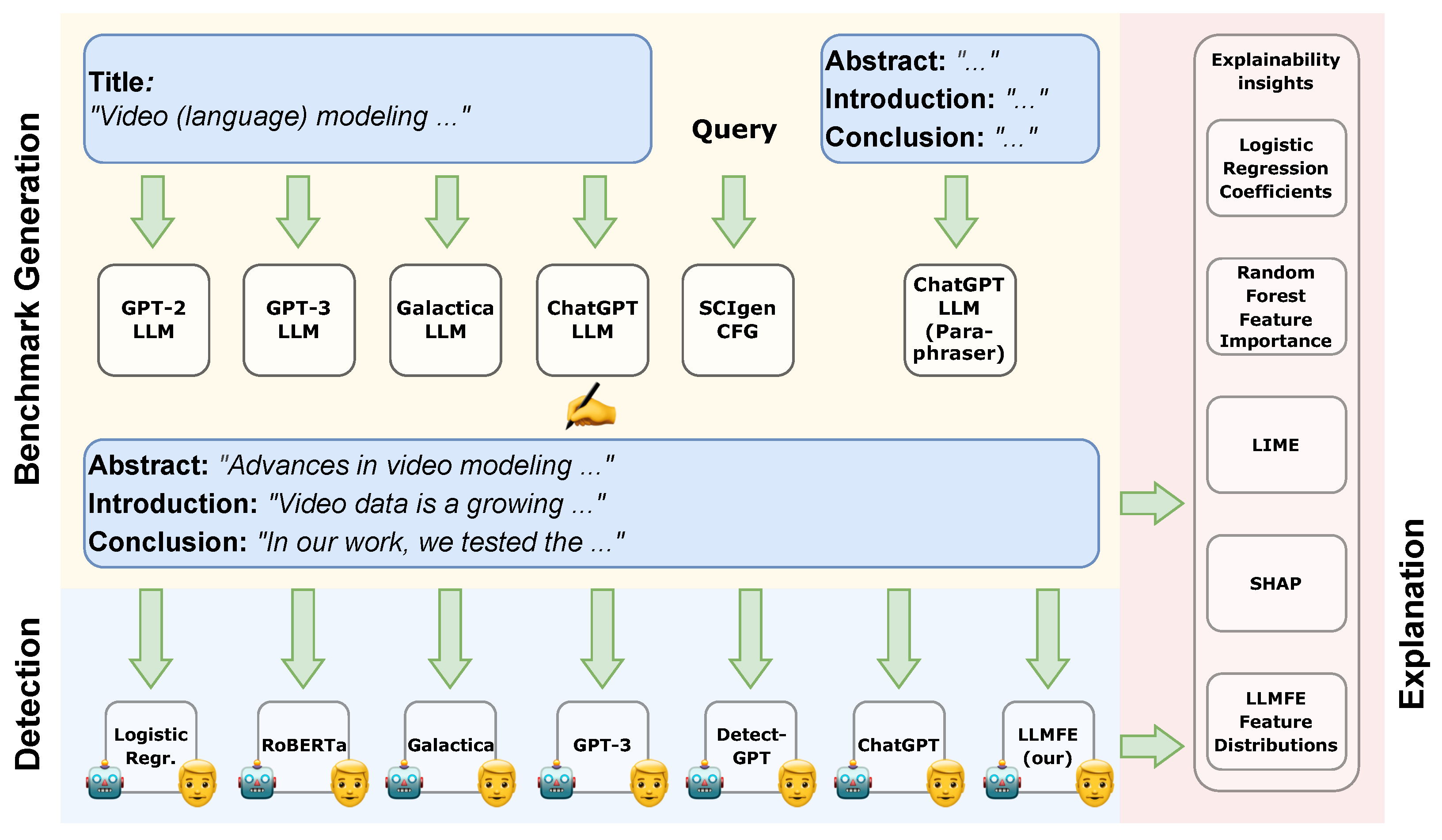
Figure 1. This work’s overview. Six methods are used to machine-generate papers, which are then mixed with human-written ones to create our benchmark dataset. Seven models are then tested as baselines to identify the authorship of a given output.
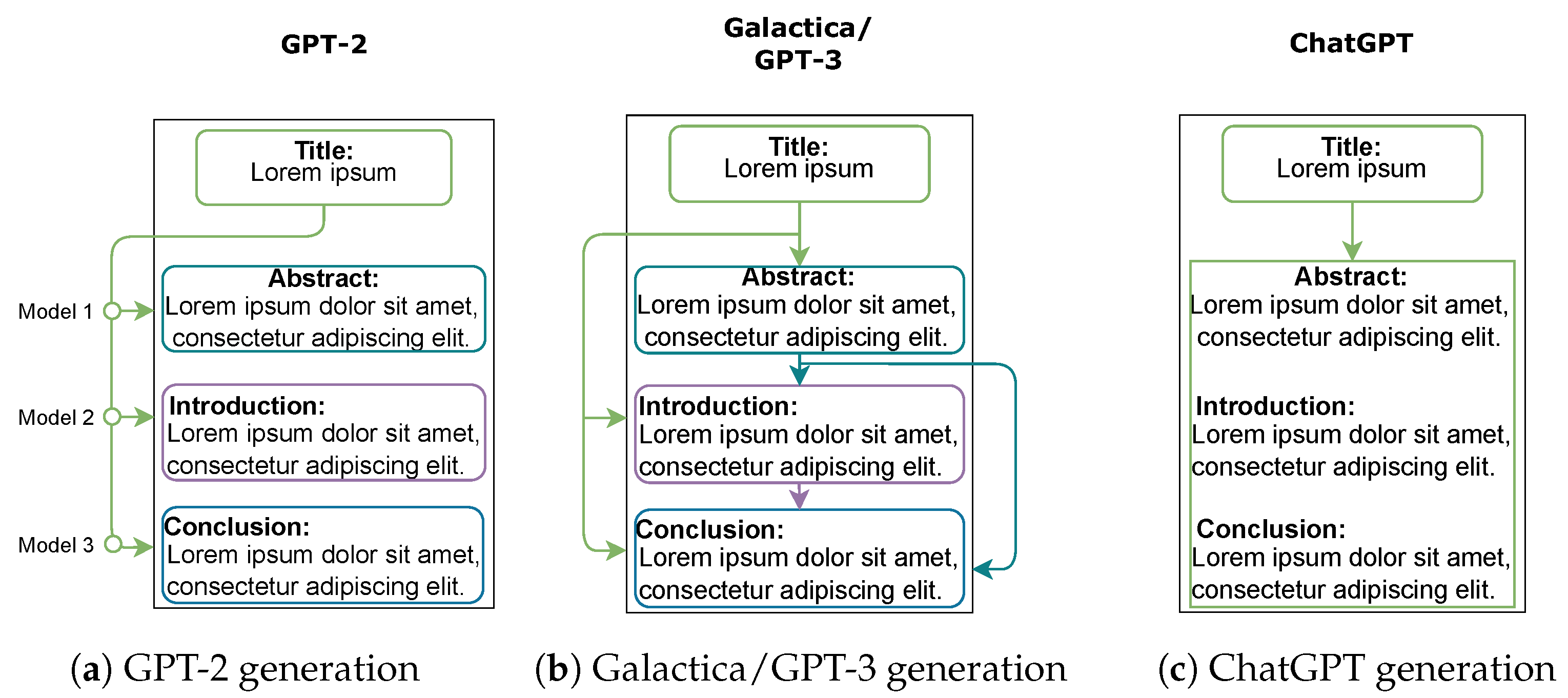
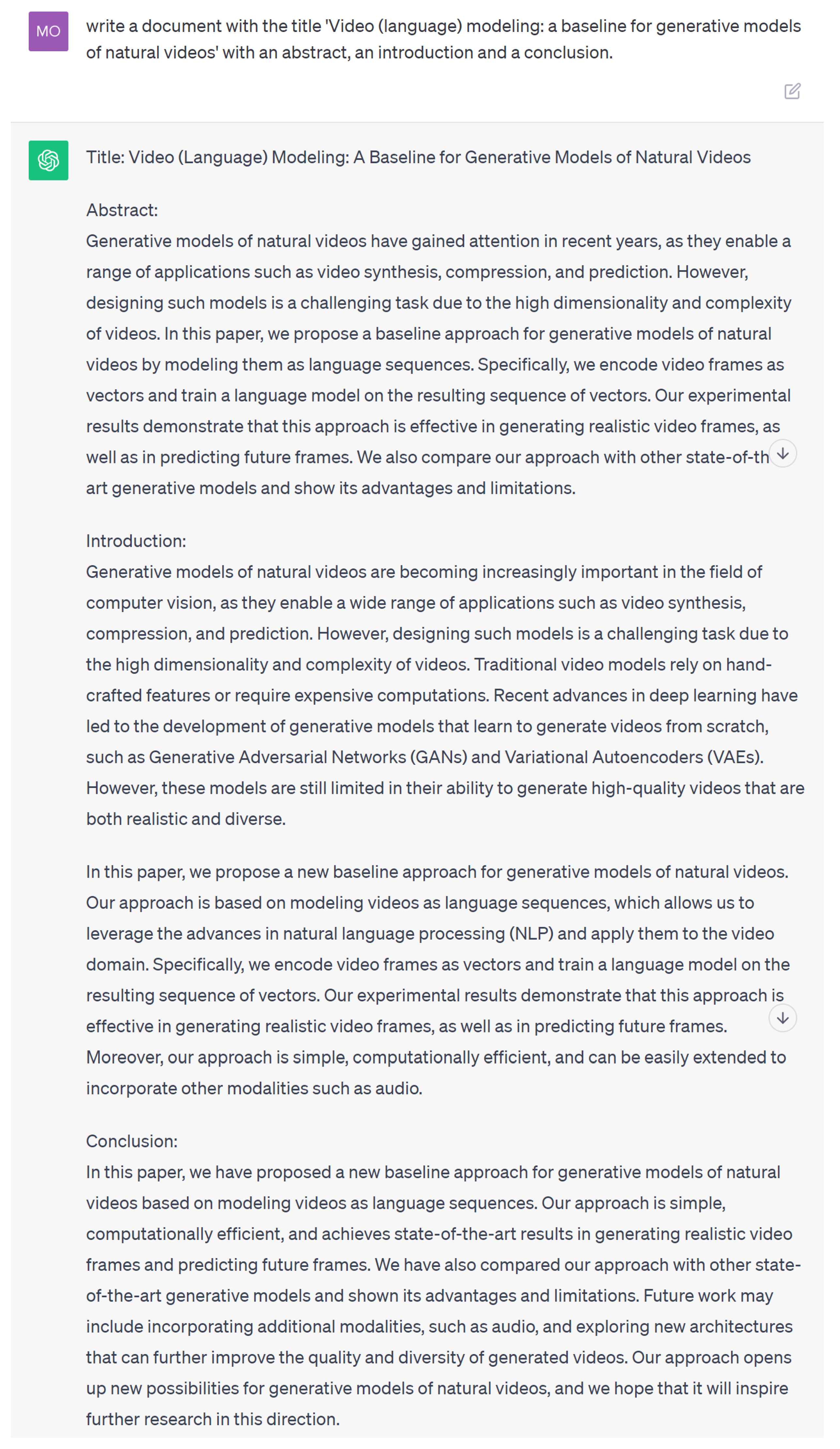
Information 14 00522 g001
Figure 2. Generation pipeline used for each model. For GPT-2 (a), the abstract, introduction, and conclusion sections are generated by three separately fine-tuned model instances, each based solely on the paper title. In the case of Galactica and GPT-3 (b), each section is generated conditioning on the previous sections. Finally, ChatGPT’s generation sequence (c) requires only the title to generate all the necessary sections at once.
Information 14 00522 g002
Figure 3. Our co-created test dataset TEST-CC contains 4000 papers with varying shares of real and ChatGPT-paraphrased sections.
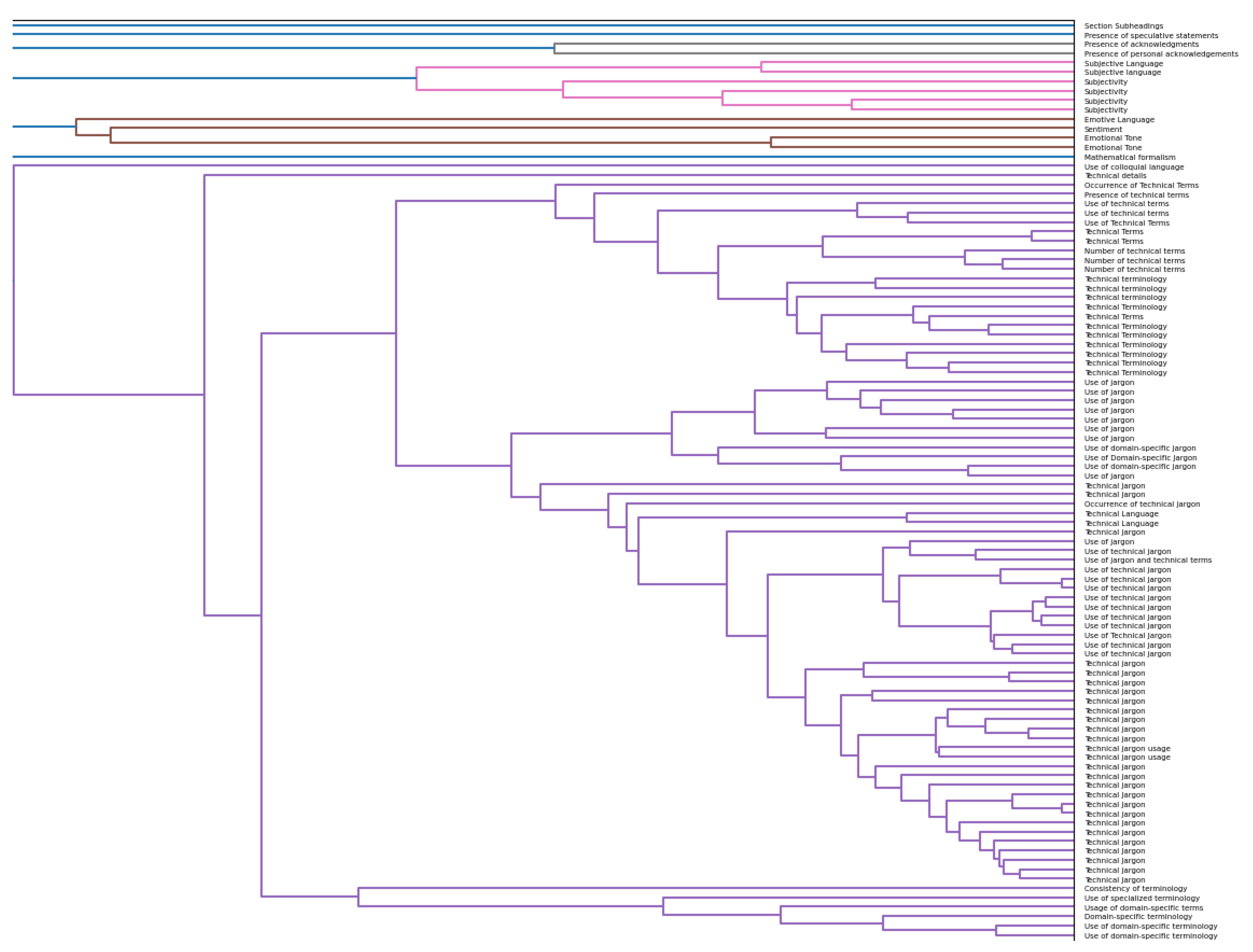
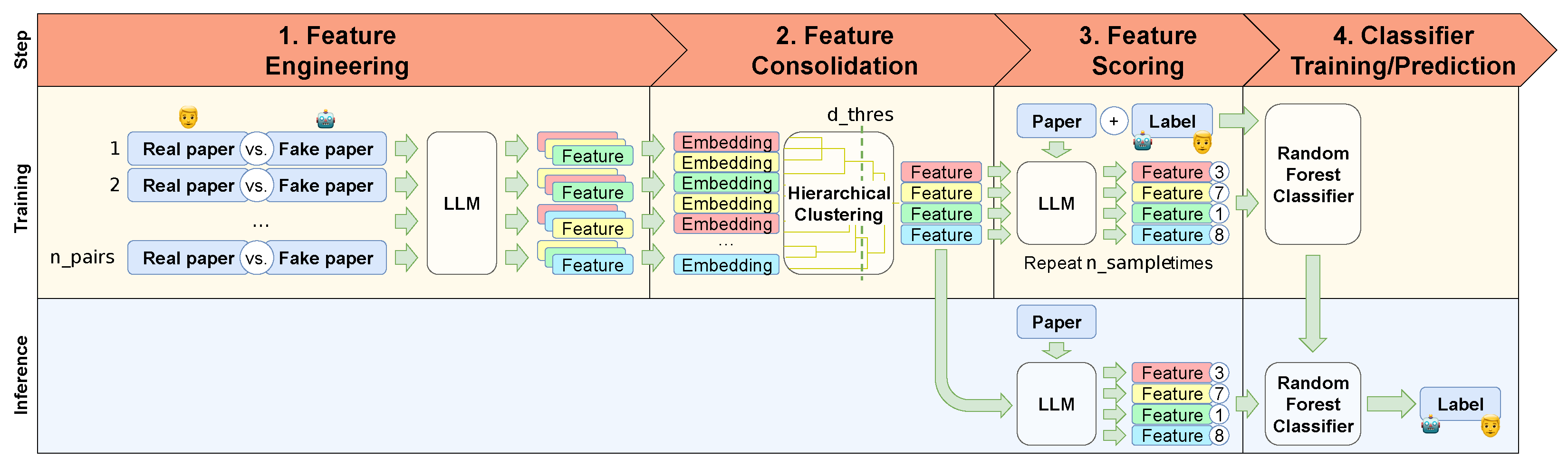
Information 14 00522 g003
Figure 4. LLMFE follows a four-step process: (1) Generate features suitable for distinguishing real and fake papers using the LLM based on multiple pairs of one real and one fake paper each. (2) Remove duplicate features through hierarchical clustering on embeddings of the feature descriptions. (3) Score scientific papers along the remaining features using the LLM. (4) Finally, train a Random Forest Classifier to predict the real or fake label based on the feature scores.
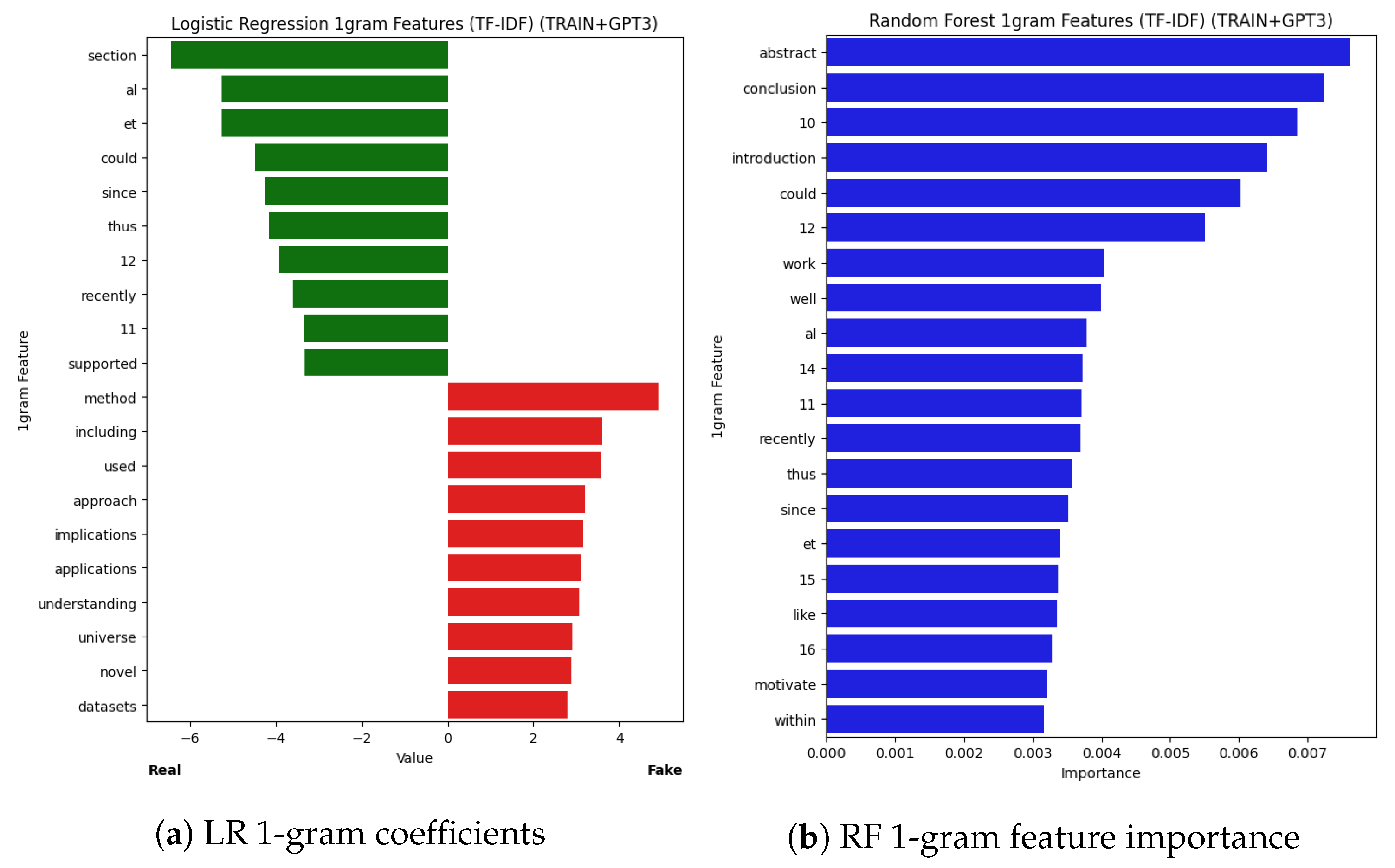
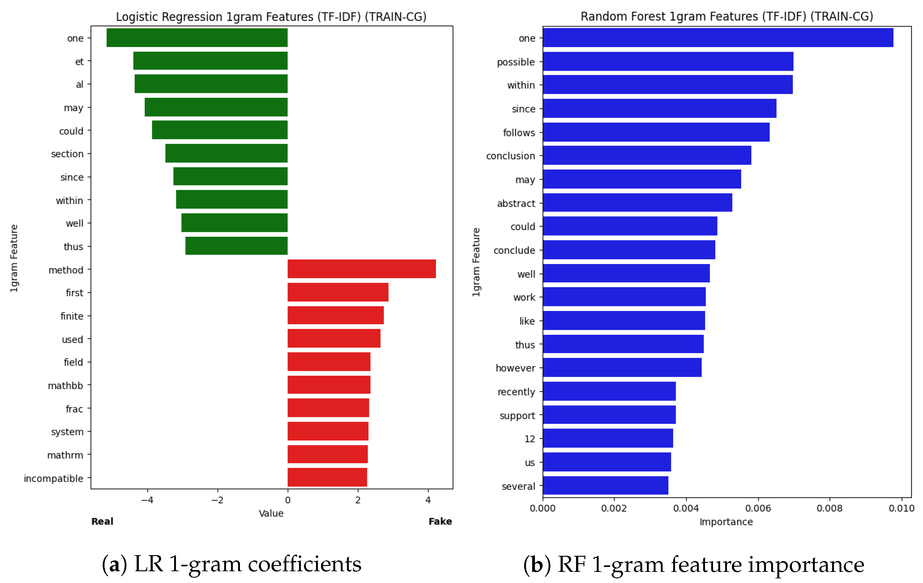
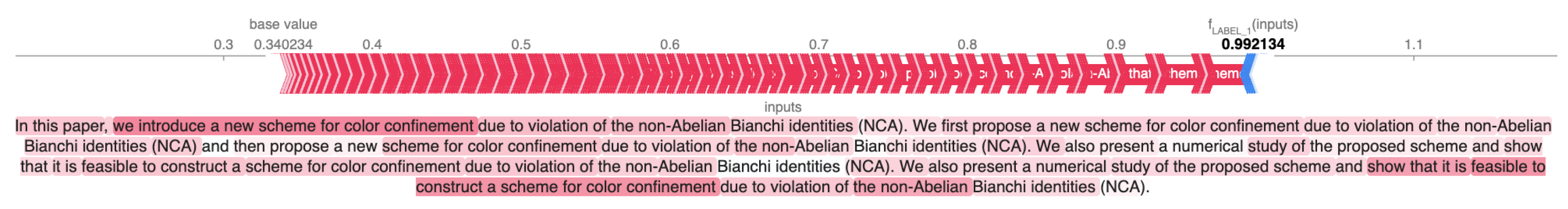
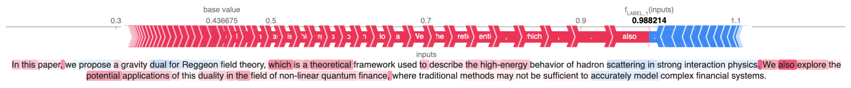
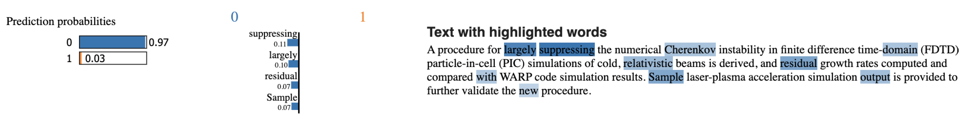
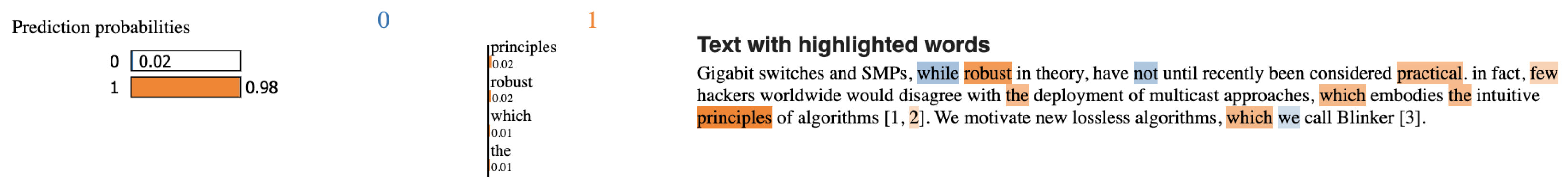
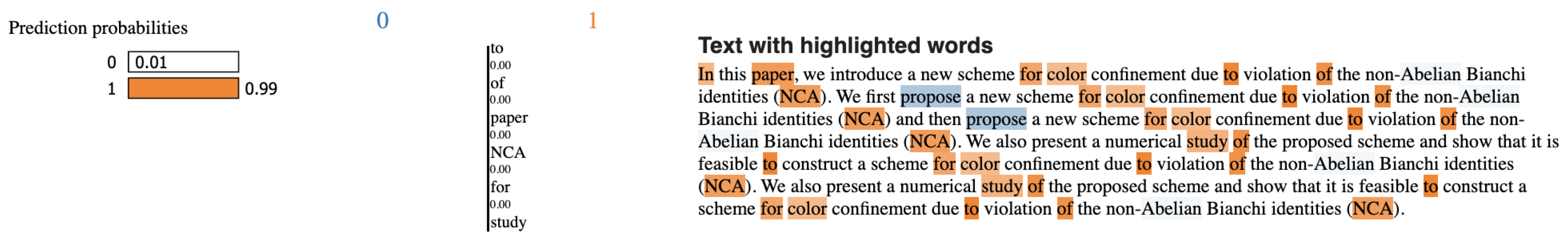
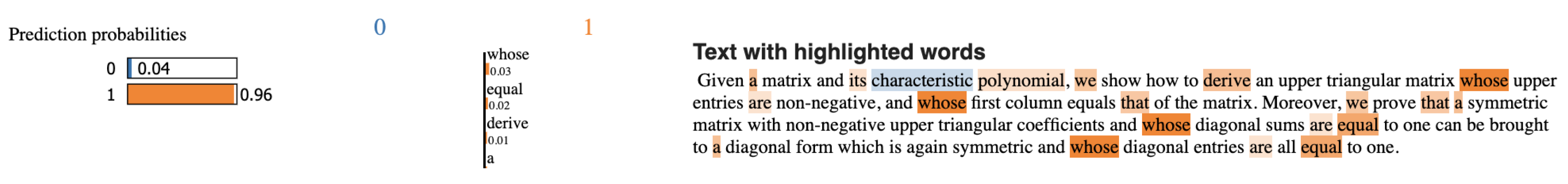
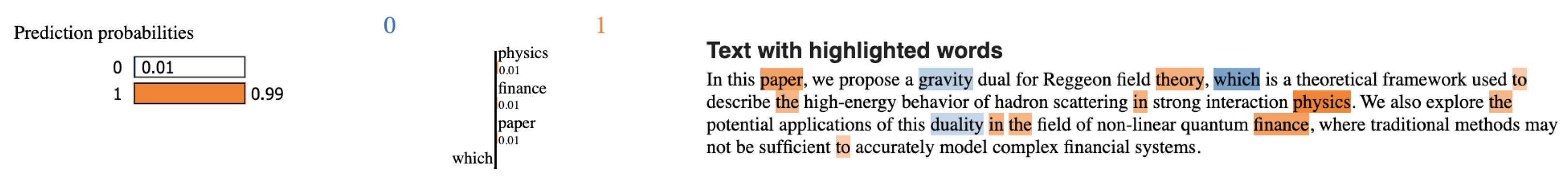
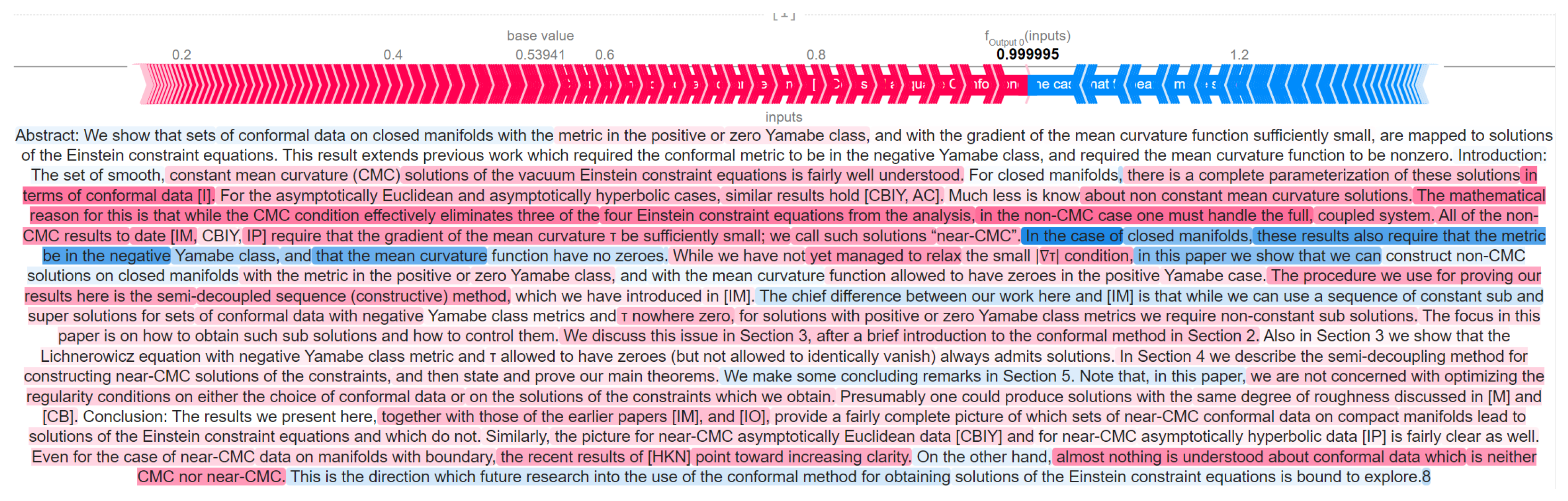
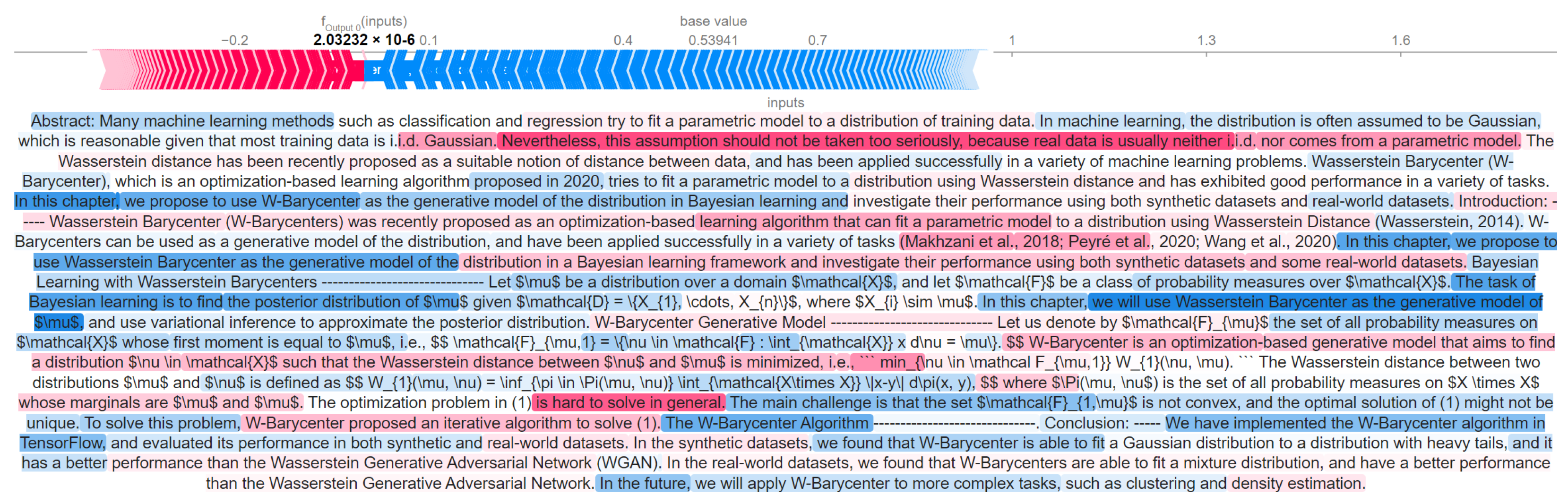
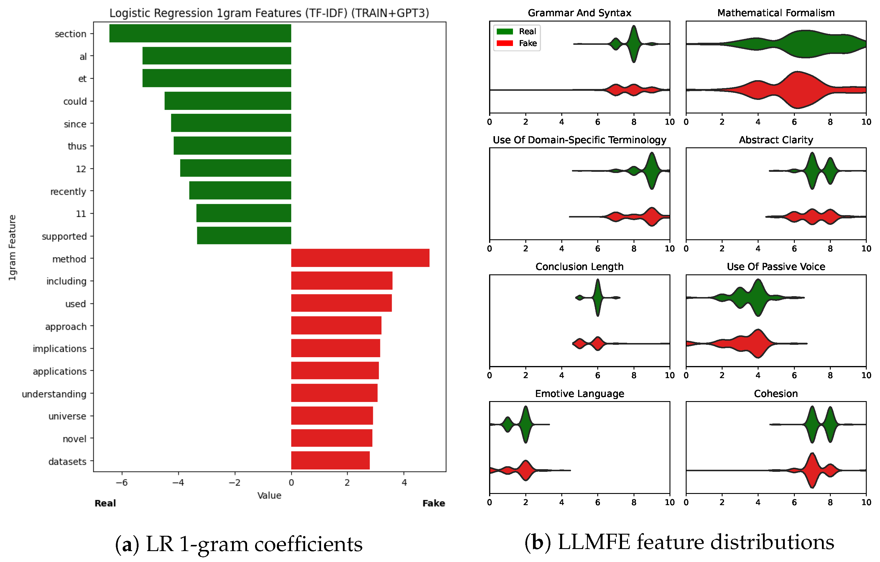
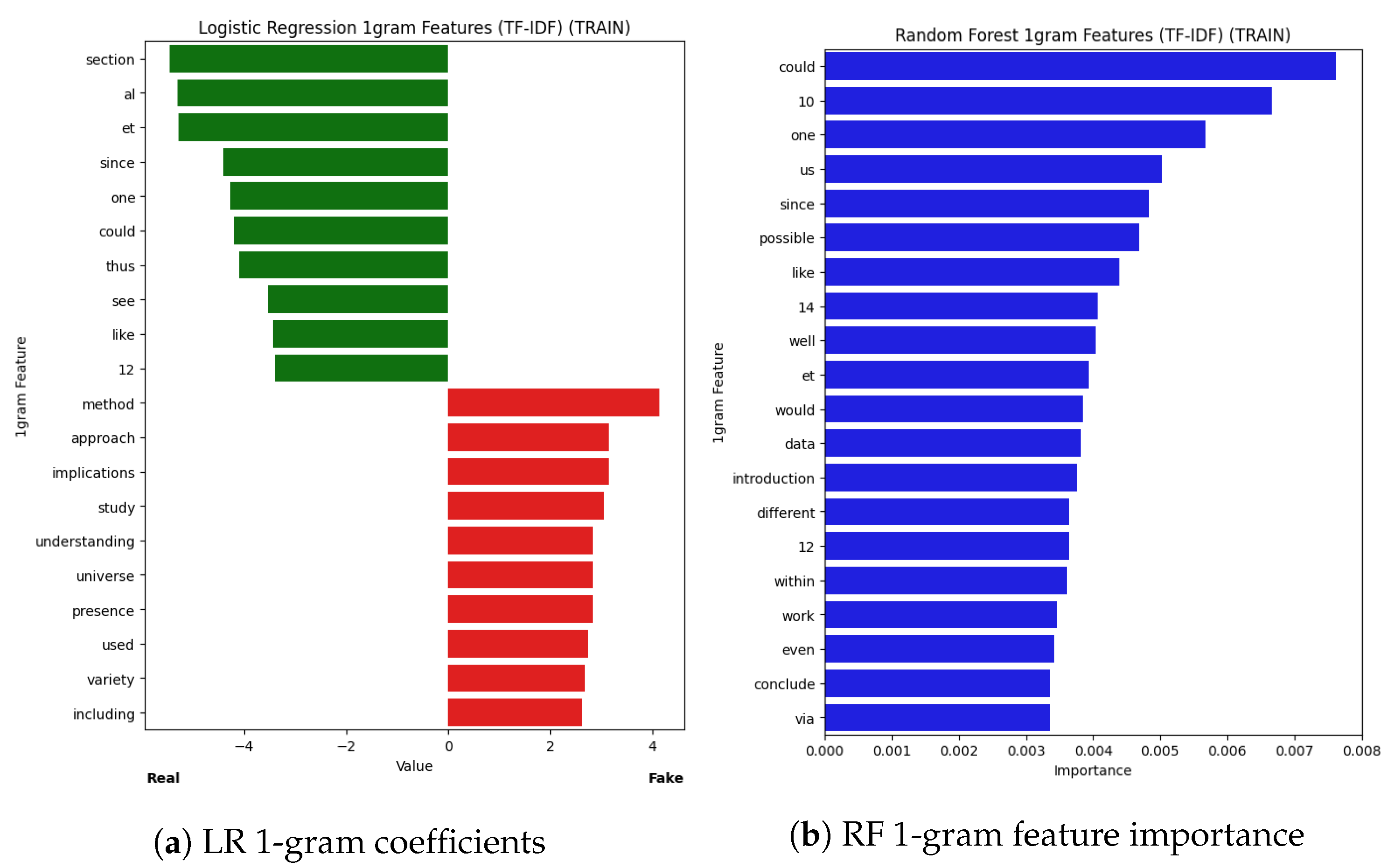
Information 14 00522 g004
Figure 5. Explainability insights from our Logistic Regression (LR) and Large Language Model Feature Extractor (LLMFE) classifiers. (a) shows the 1-grams with the 10 lowest (indicating real) and highest (indicating fake) coefficients learned by LR. (b) shows the distributions of scores for the eight most important features (according to Random Forest feature importance) learned by LLMFE.
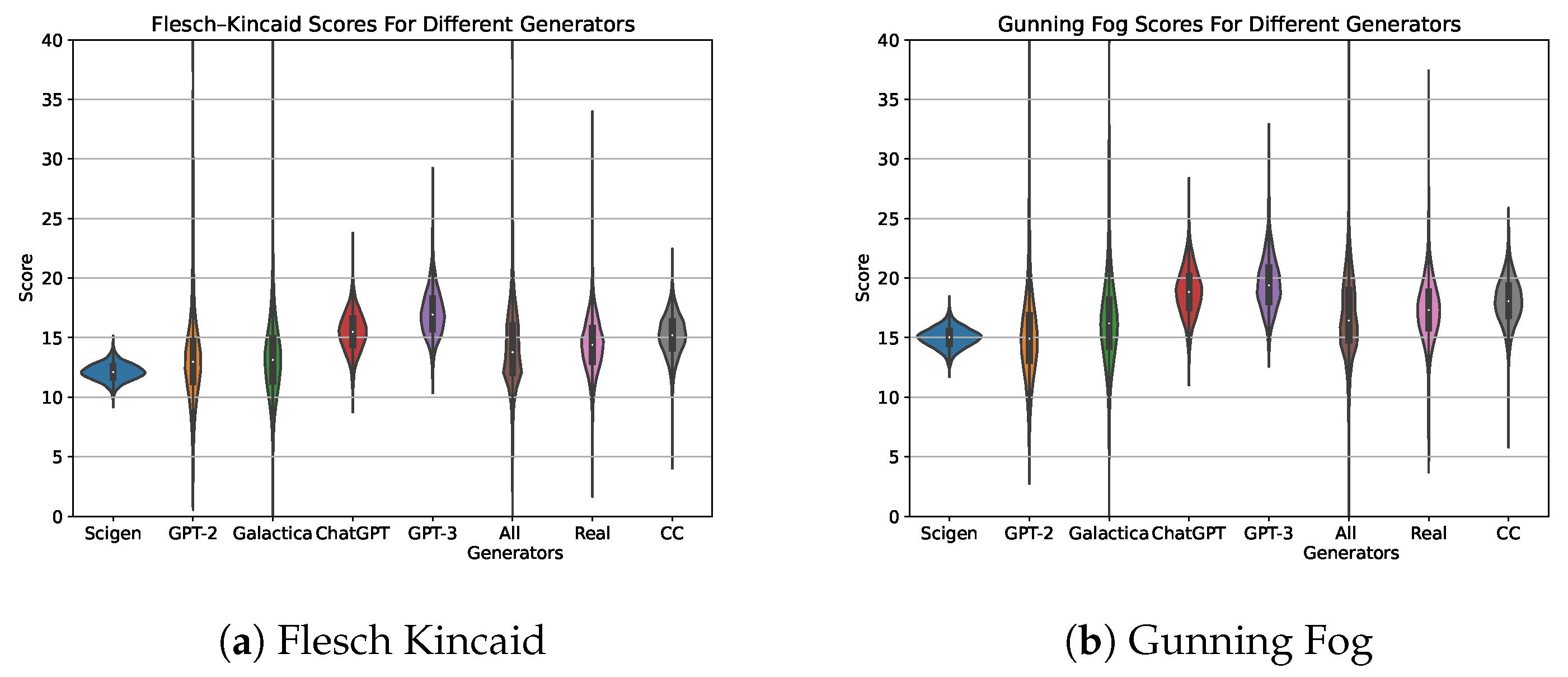
Information 14 00522 g005
Figure 6. Distribution of readability metrics for papers from the different generators. (a) shows Flesch–Kincaid scores while (b) shows Gunning Fog scores for all generators.
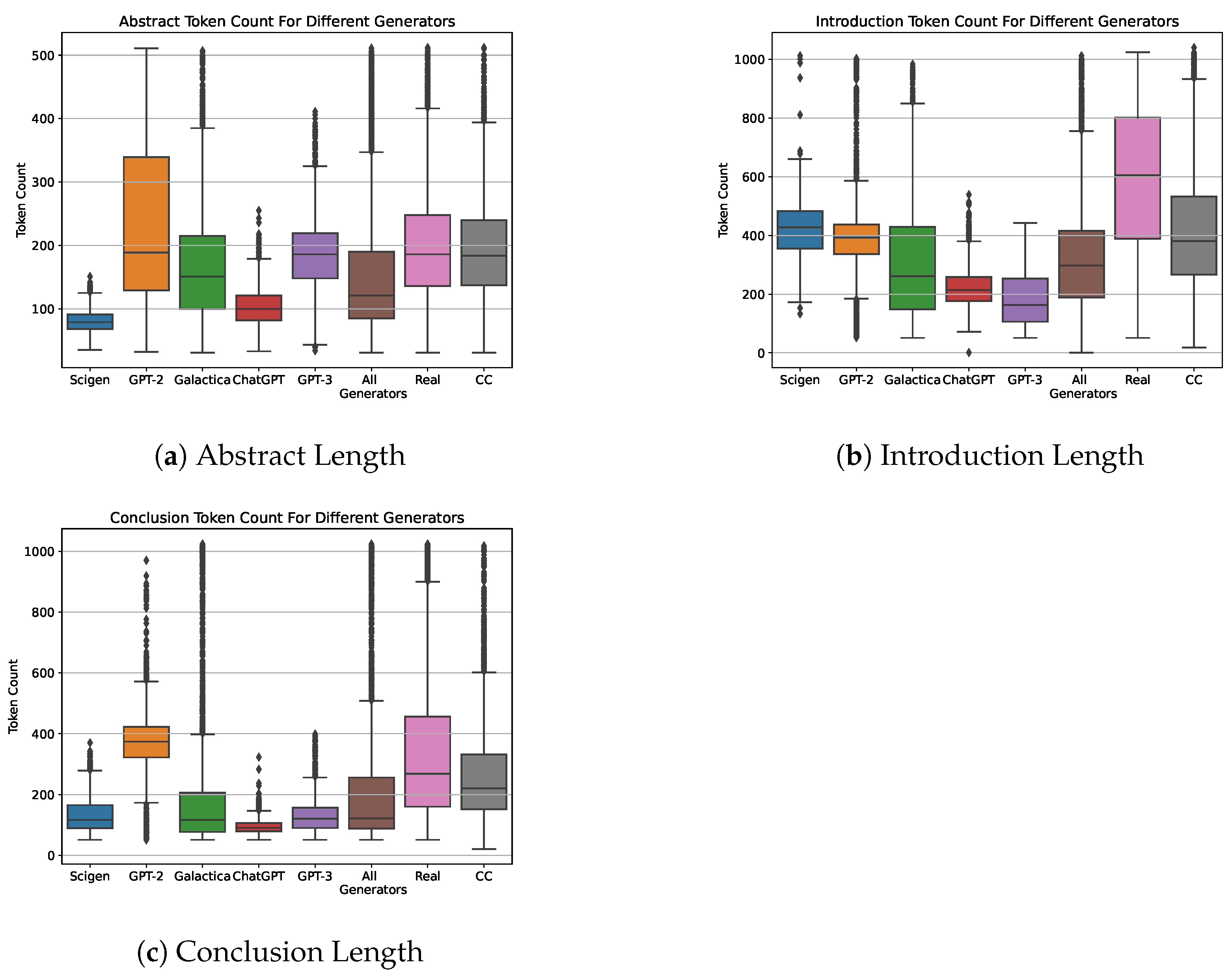
Information 14 00522 g006
Figure 7. The generators exhibit different tendencies for the length of the generated fake scientific papers. (a) shows the length distribution of generated abstracts, (b) shows the same for introductions, and (c) shows conclusion lengths.
Information 14 00522 g007
Figure 8. Paraphrasing sections with ChatGPT has a tendency to result in sections shorter than the original. The reduction in section length is most visible for the longer introduction and conclusion sections. For an analysis of lengths of generated fake scientific papers, see Figure 7 in the appendix.
Information 14 00522 g008
Table 1. Data sources included in our dataset and their respective sizes.
SourceQuantityTokens
arXiv parsing 1 (real)12 k13.4 M
arXiv parsing 2 (real)4 k3.2 M
SCIgen (fake)3 k1.8 M
GPT-2 (fake)3 k2.9 M
Galactica (fake)3 k2.0 M
ChatGPT (fake)3 k1.2 M
GPT-3 (fake)1 k0.5 M
ChatGPT (paraphrased real)4 k3.5 M
Total real (extraction)16 k16.6 M
Total fake (generators)13 k8.4 M
Total co-created (paraphrased)4 k3.5 M
Total33 k28.5 M
Table 2. Overview of the datasets used to train and evaluate the classifiers. Each column represents the number of papers used per source. Concerning real papers, unless indicated, we use samples extracted with parsing 1 (see Section 3.1).
arXivChatGPTGPT-2SCIgenGalacticaGPT-3ChatGPT
Dataset(Real)(Fake)(Fake)(Fake)(Fake)(Fake)(Co-Created)
Standard train (TRAIN)8 k2 k2 k2 k2 k--
Standard train subset (TRAIN-SUB)4 k1 k1 k1 k1 k--
TRAIN without ChatGPT (TRAIN-CG)8 k-2 k2 k2 k--
TRAIN plus GPT-3 (TRAIN + GPT3)8 k2 k2 k2 k2 k1.2 k-
Standard test (TEST)4 k1 k1 k1 k1 k--
Out-of-domain GPT-3 only (OOD-GPT3)-----1 k-
Out-of-domain real (OOD-REAL)4 k (parsing 2)------
ChatGPT only (TECG)-1 k-----
Co-created test (TEST-CC)------4 k
Table 3. Experiment results reported with accuracy metric. Out-of-domain experiments, i.e., evaluation on unseen generators, are highlighted in blue. Highest values per test set are highlighted in bold. (*) ChatGPT-IO and LLMFE accuracies have been evaluated on randomly sampled subsets of 100 scientific papers per test set due to API limits.
ModelTrain DatasetTESTOOD-GPT3OOD-REALTECGTEST-CC
LR-1gram (tf-idf) (our)TRAIN95.3%4.0%94.6%96.1%7.8%
LR-1gram (tf-idf) (our)TRAIN + GPT394.6%86.5%86.2%97.8%13.7%
LR-1gram (tf-idf) (our)TRAIN-CG86.6%0.8%97.8%32.6%1.2%
RF-1gram (tf-idf) (our)TRAIN94.8%24.7%87.3%100.0%8.1%
RF-1gram (tf-idf) (our)TRAIN + GPT391.7%95.0%69.3%100.0%15.1%
RF-1gram (tf-idf) (our)TRAIN-CG97.6%7.0%95.0%57.0%1.7%
Galactica (our)TRAIN98.4%25.9%95.5%84.0%6.8%
Galactica (our)TRAIN + GPT398.5%71.2%95.1%84.0%12.0%
Galactica (our)TRAIN-CG96.4%12.4%97.6%61.3%2.4%
RoBERTa (our)TRAIN72.3%55.5%50.0%100.0%63.5%
RoBERTa (our)TRAIN + GPT365.7%100.0%29.1%100.0%75.0%
RoBERTa (our)TRAIN-CG86.0%2.0%92.5%76.5%9.2%
GPT-3 (our)TRAIN-SUB100.0%25.9%99.0%100.0%N/A
DetectGPT-61.5%0.0%99.9%68.7%N/A
ChatGPT-IO (our) (*)-69.0%49.0%89.0%0.0%3.0%
LLMFE (our) (*)TRAIN + GPT380.0%62.0%70.0%90.0%33.0%
Disclaimer/Publisher’s Note: The statements, opinions and data contained in all publications are solely those of the individual author(s) and contributor(s) and not of MDPI and/or the editor(s). MDPI and/or the editor(s) disclaim responsibility for any injury to people or property resulting from any ideas, methods, instructions or products referred to in the content.

