


A Closer Look at Machine Learning Effectiveness in Android Malware Detection


Abstract
1. Introduction
- A large dataset of contemporary malware is collected to extract features using static analysis;
- Twenty seven different ML models were trained, using the aforementioned dataset in an effort to find the best performer;
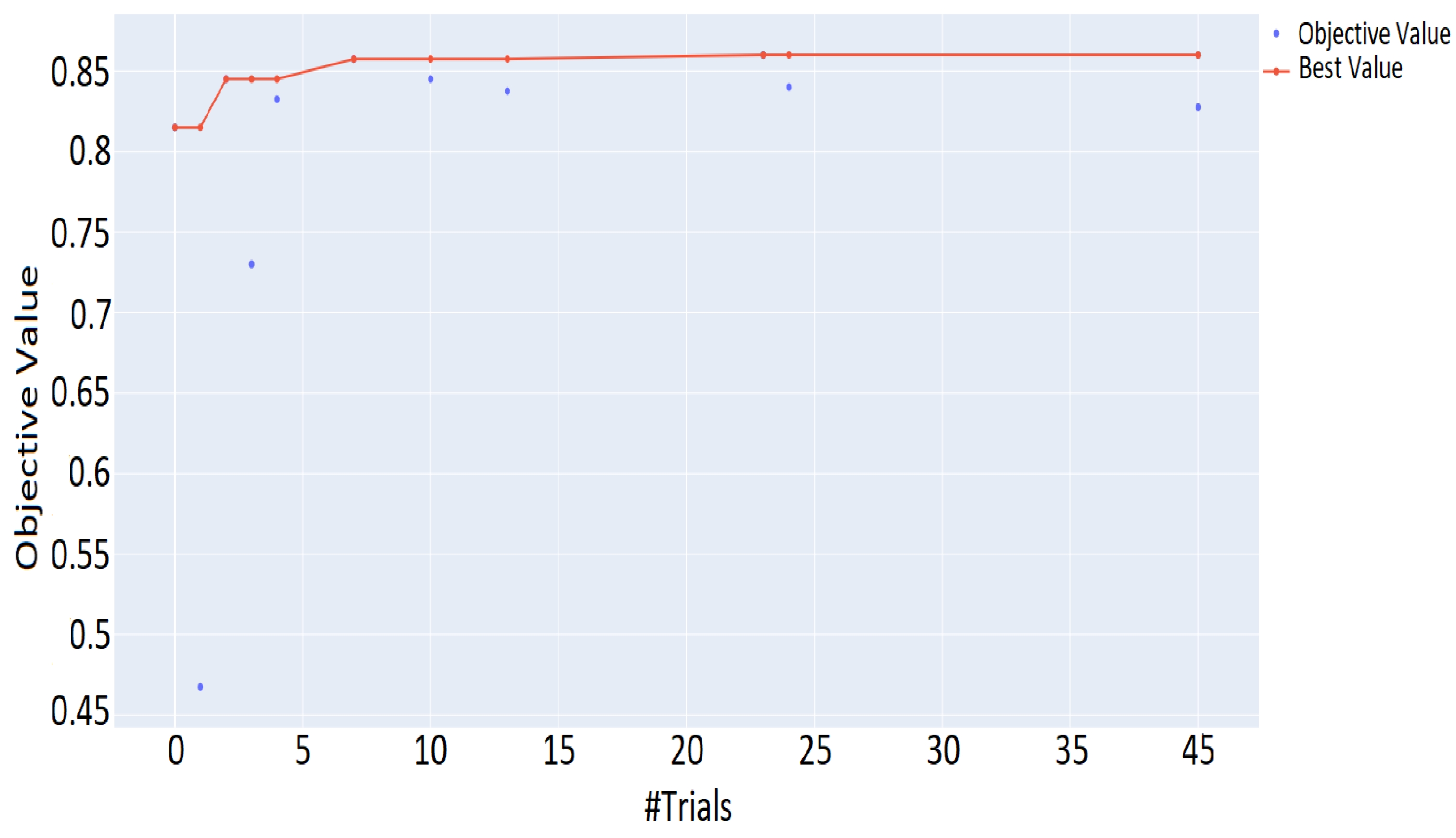
- A DNN model is tuned and optimized after conducting hyperparameters importance analysis, by using the Optuna framework on our benchmark dataset.
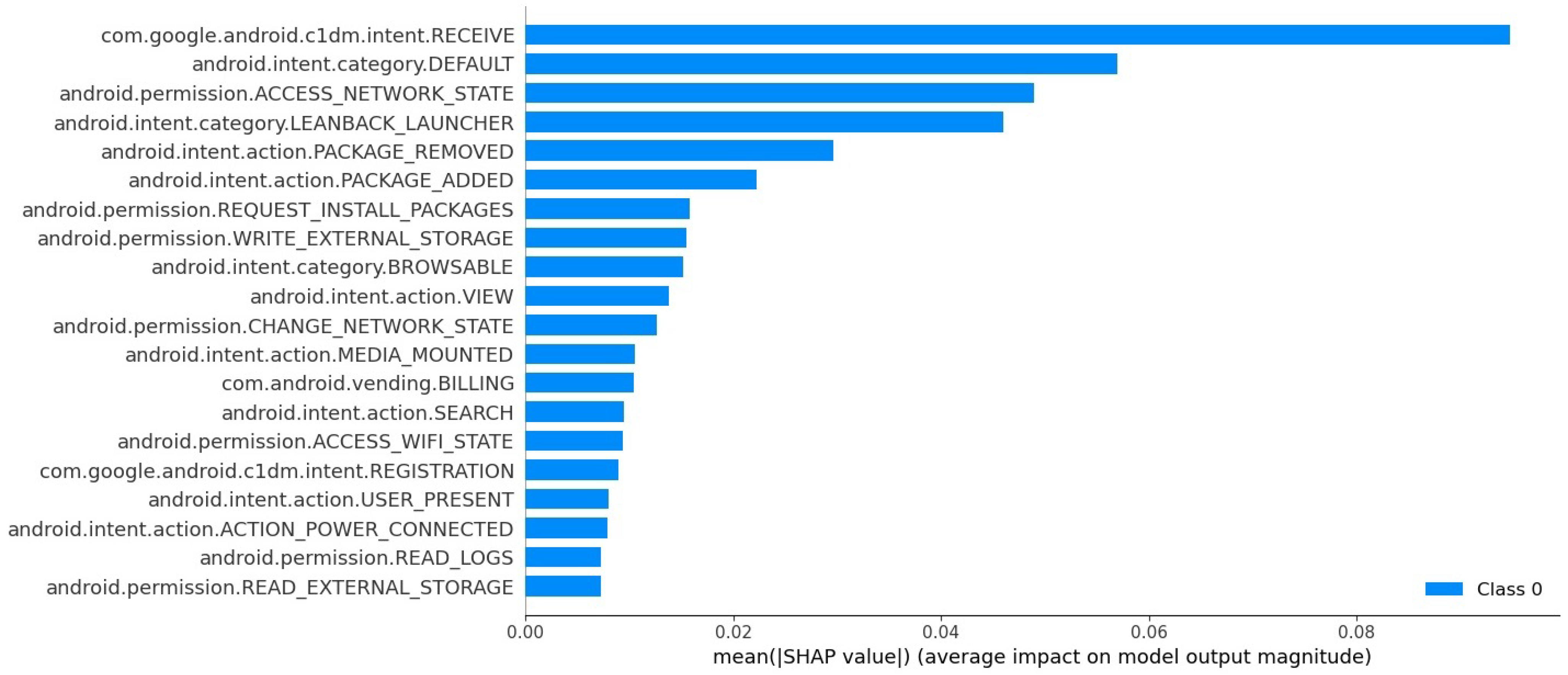
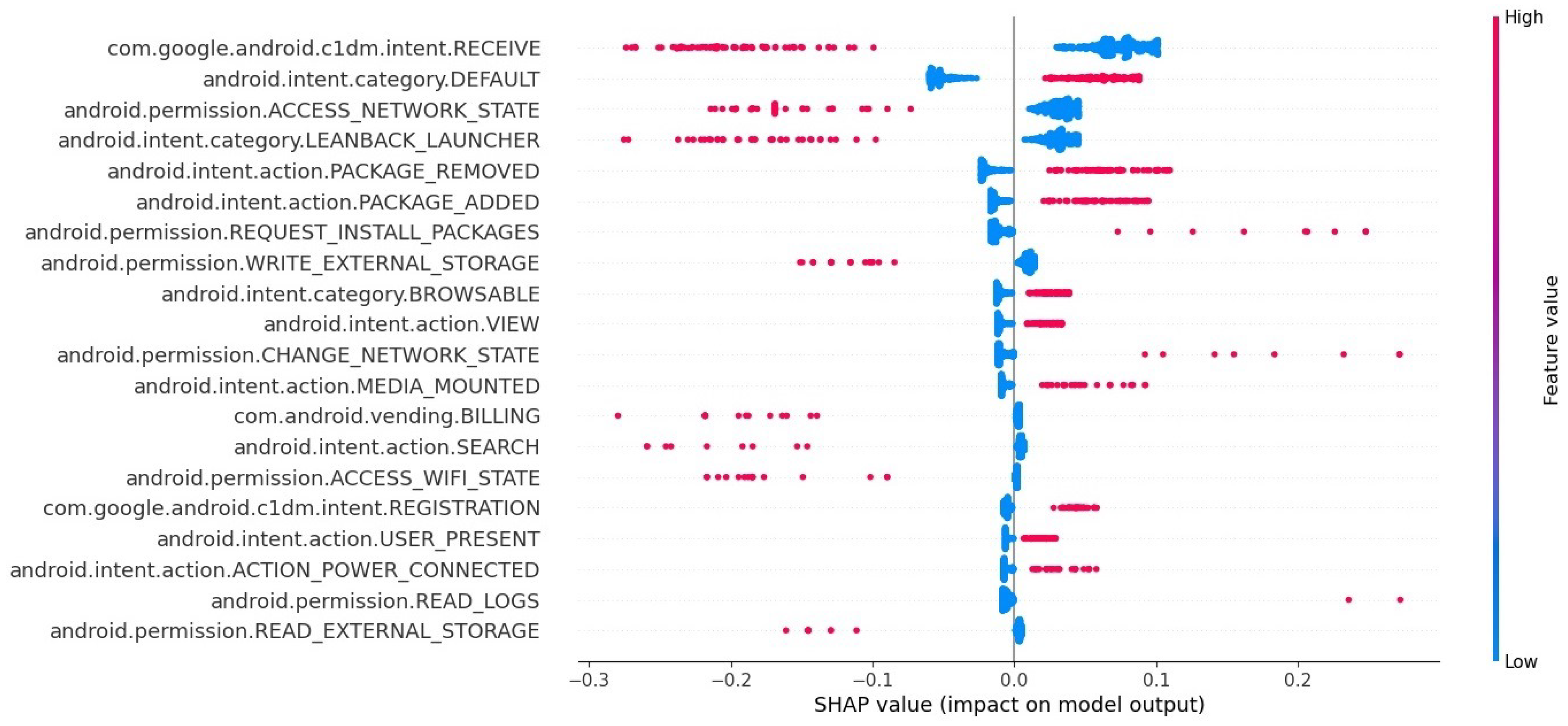
- Feature importance analysis is performed using the SHAP framework on the best performing ML model to reveal the most significant classification features.
2. Related Work

| Work | Year | Models Compared | Model Optimization | Hyperparameters Tuning | Feature Importance | Contemporary Dataset |
|---|---|---|---|---|---|---|
| [7] | 2018 | - | - | - | - | - |
| [9] | 2018 | - | - | - | - | - |
| [11] | 2018 | - | - | - | - | - |
| [12] | 2018 | - | - | - | - | - |
| [14] | 2018 | - | - | - | - | - |
| [17] | 2018 | - | - | - | - | - |
| [19] | 2019 | - | - | - | - | - |
| [20] | 2020 | - | - | - | - | - |
| [21] | 2020 | 8 | - | - | - | + |
| [23] | 2020 | - | - | + | - | - |
| [24] | 2020 | - | - | + | - | - |
| [28] | 2021 | - | - | + | - | - |
| [29] | 2021 | - | - | + | - | - |
| [30] | 2021 | - | - | - | + | - |
| [31] | 2021 | - | - | - | - | - |
| [32] | 2022 | 12 | + | + | + | + |
| [34] | 2022 | - | + | + | + | + |
| This work | 2022 | 27 | + | + | + | + |
3. Methodology
3.1. Dataset
3.2. Data Analysis
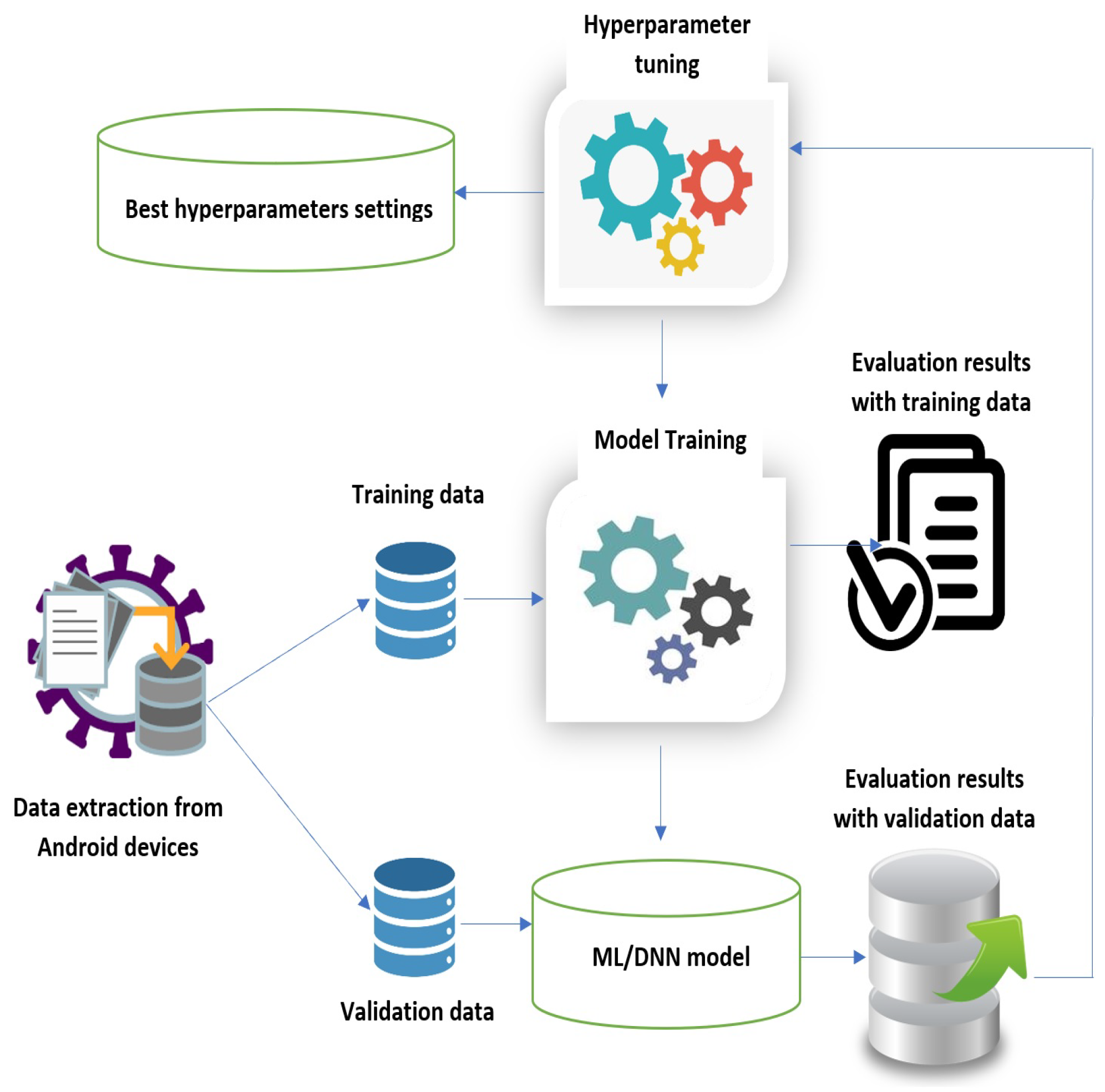
3.3. Research Design and Testbed
3.4. Performance Metrics
4. Shallow Classifiers
4.1. Initial Analysis
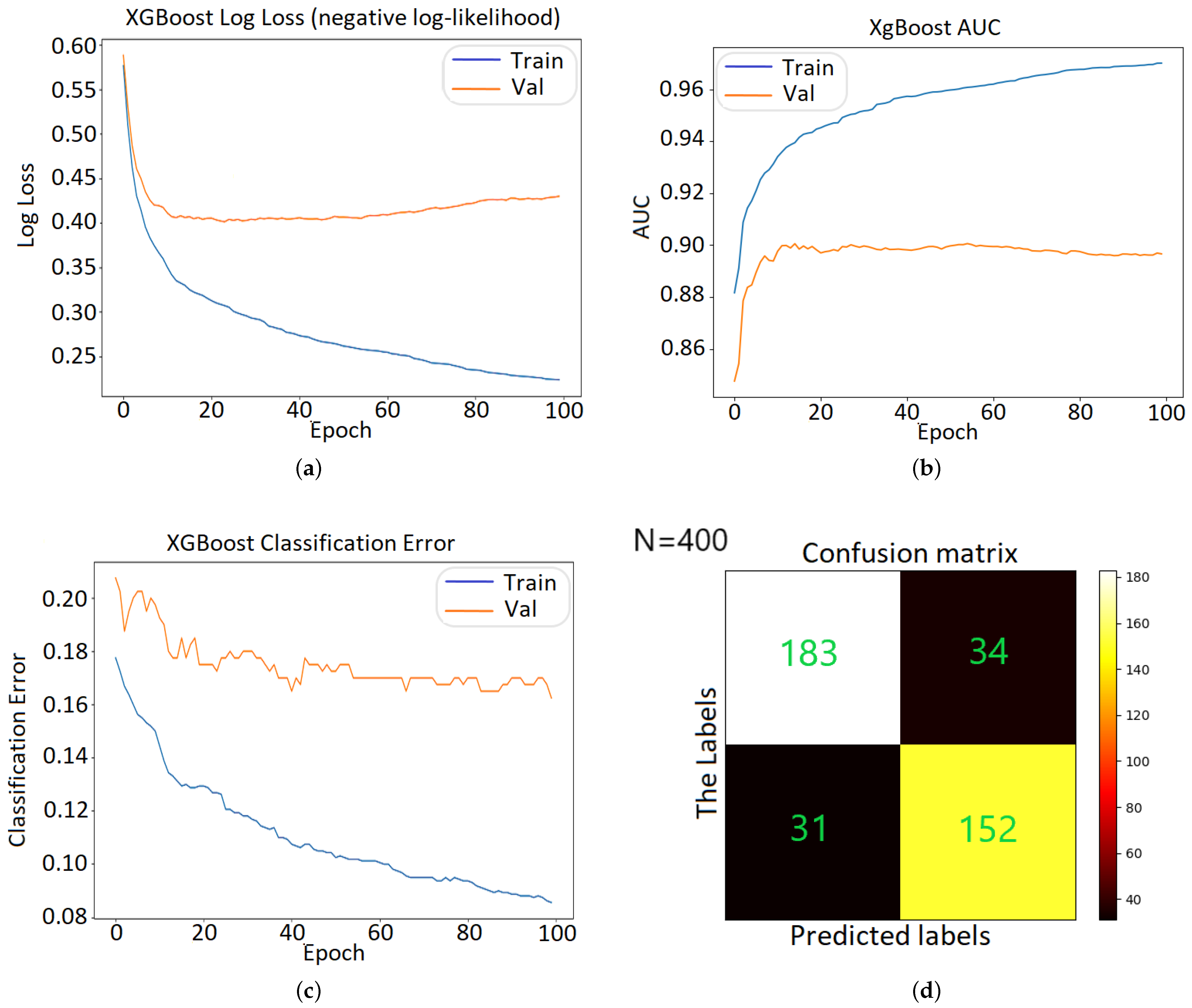
4.2. ML Optimization
5. DNN Analysis
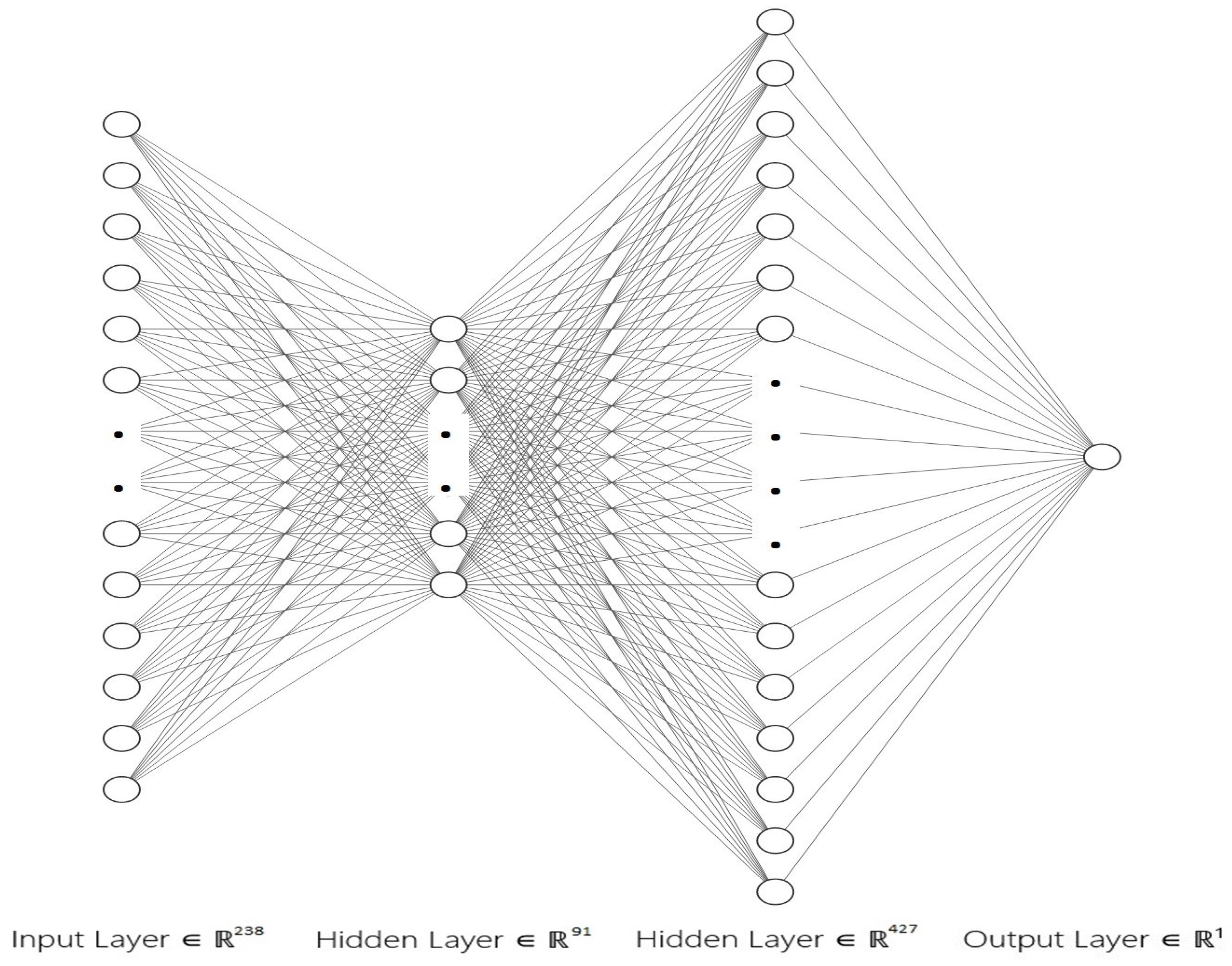
5.1. Preliminaries
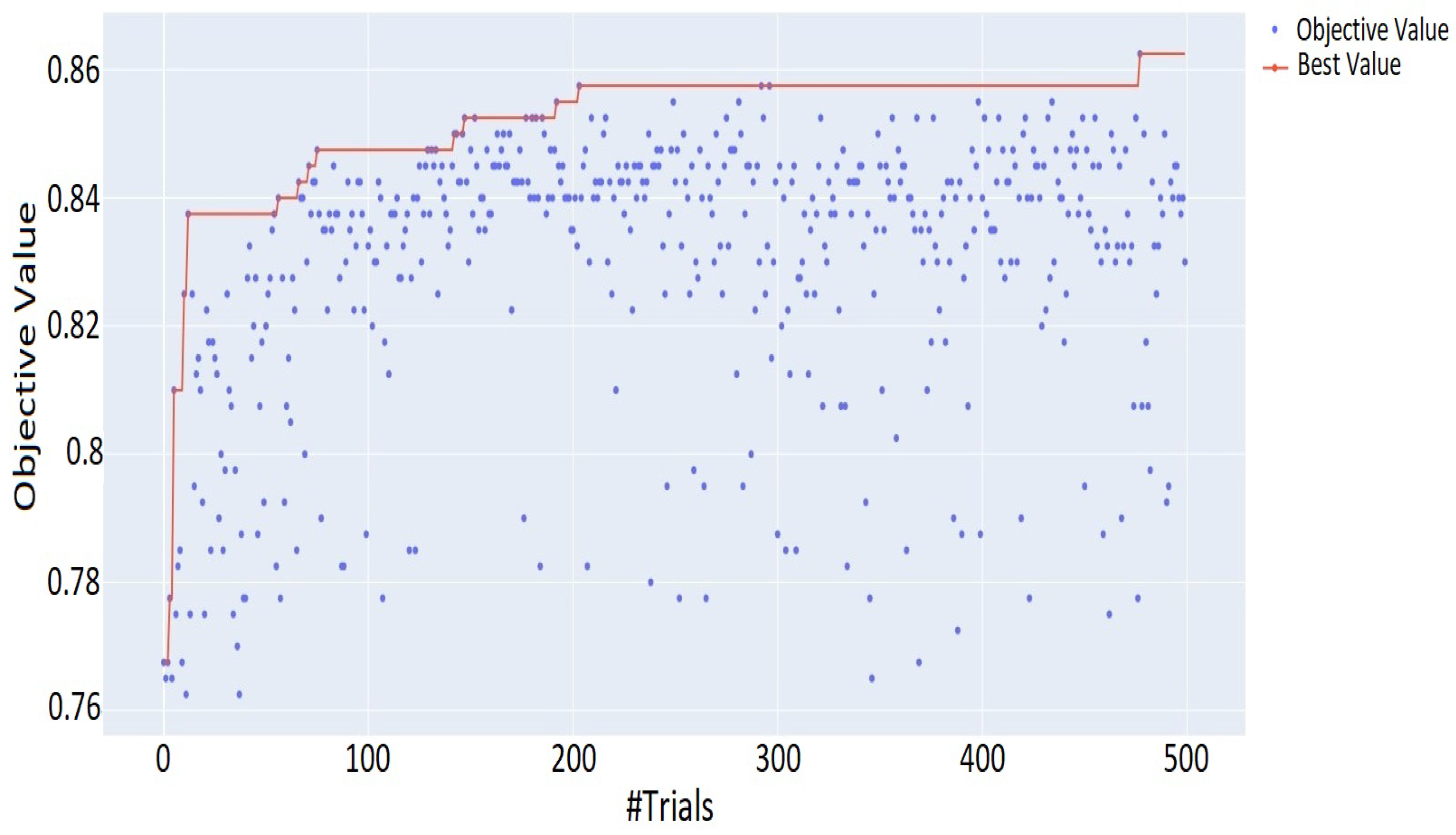
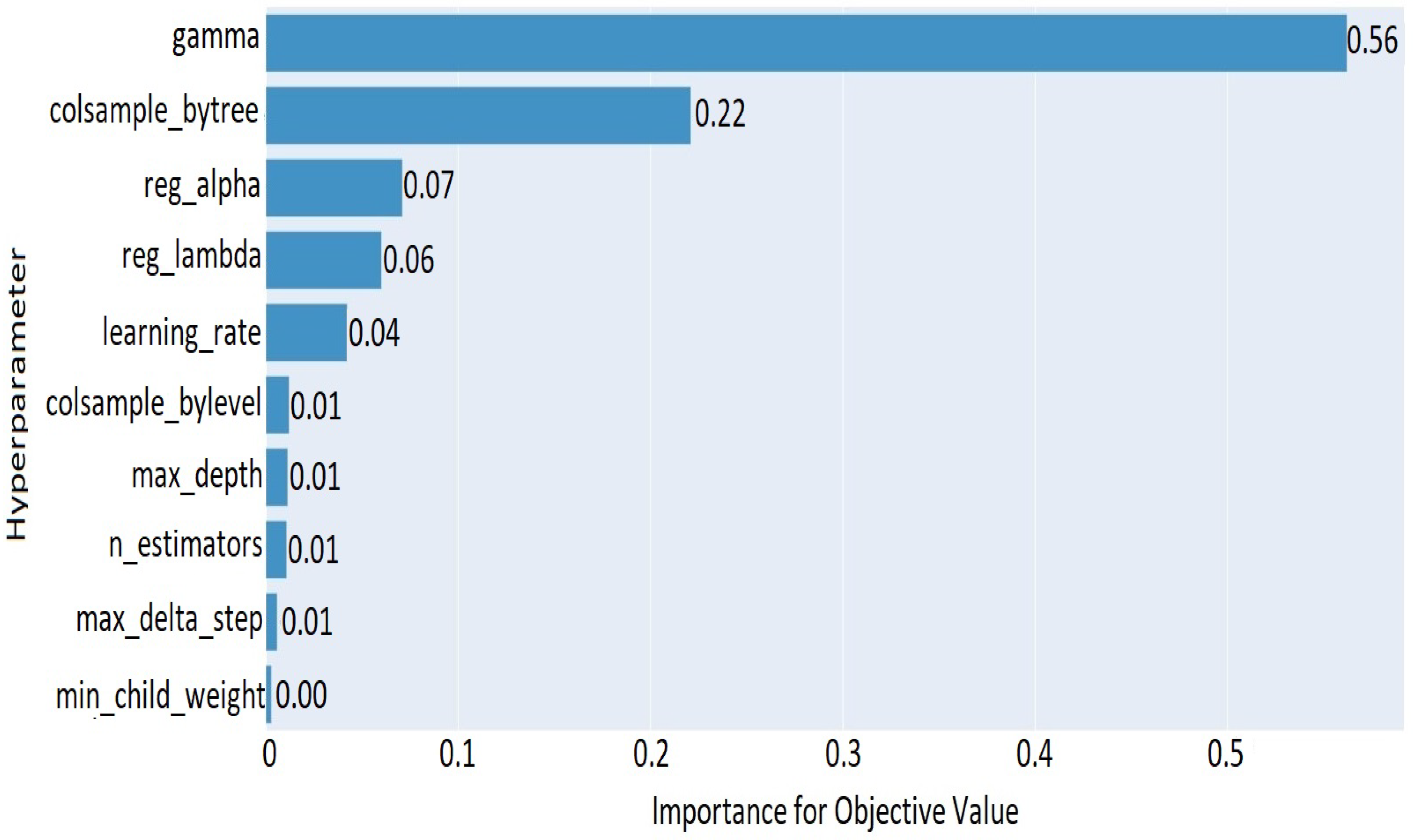
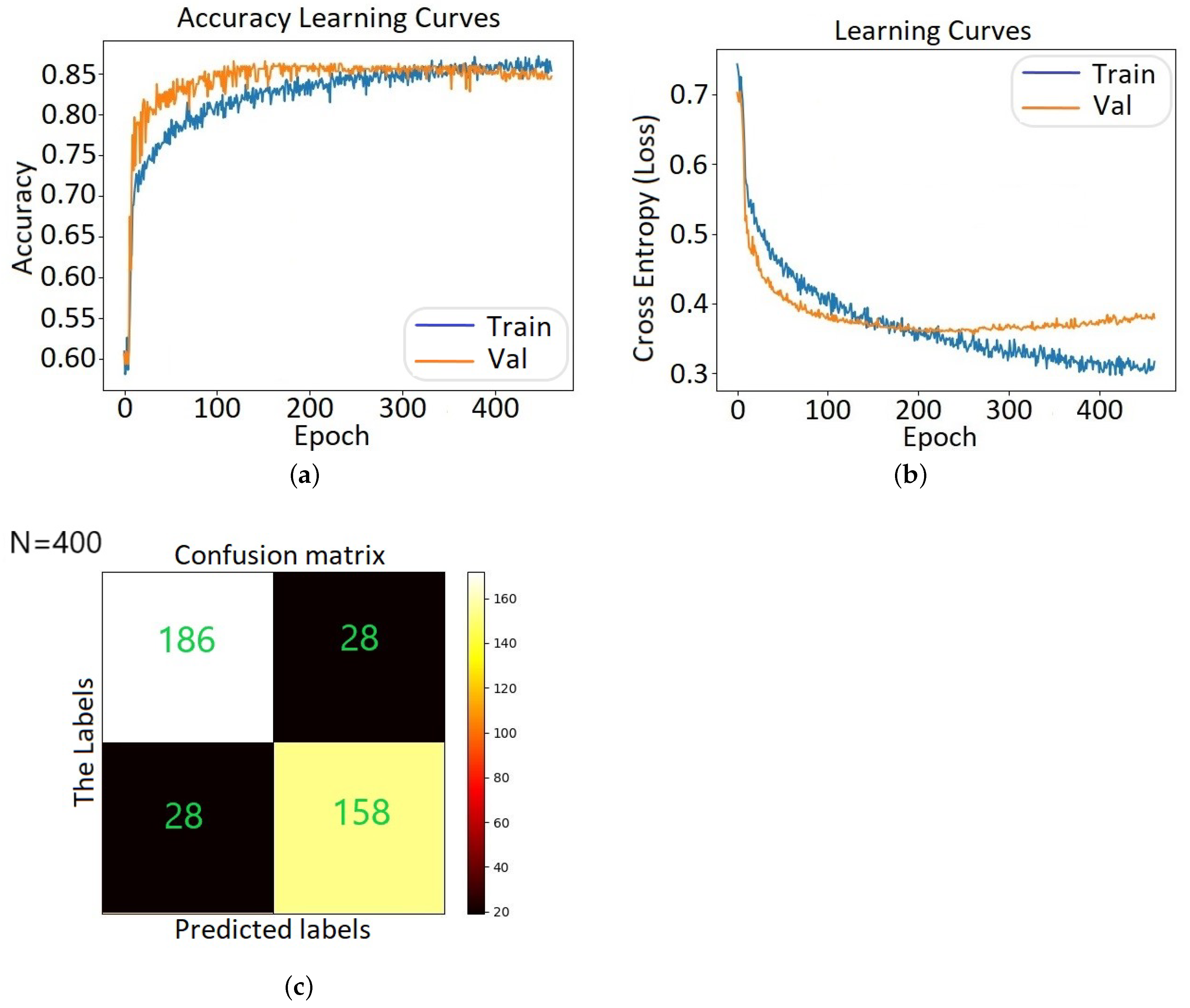
5.2. DNN Hyperparameter Optimization and Evaluation Results
6. SHAP Analysis and Features Importance Assessment
7. Conclusions
Author Contributions
Funding
Institutional Review Board Statement
Informed Consent Statement
Data Availability Statement
Conflicts of Interest
Abbreviations
| AI | Artificial Intelligent |
| AMD | Android Malware Dataset |
| APK | Android Package Kit |
| AUC-ROC | Area Under The Curve-Receiver Operating Characteristics |
| CNN | Convolutional Neural Networks |
| DNN | Deep Neural Network |
| DT | Decision Tree |
| FFN | Feed-Forward network |
| FN | False Negative |
| FPR | False Positive Rate |
| FP | False Positive |
| LR | Logistic Regression |
| LSTM | Long Short-Term Memory |
| ML | Machine Learning |
| NN | Neural Networks |
| RNN | Recurrent Neural Network |
| SHAP | Shapley Additive Explanations |
| SVM | Support Vector Machine |
| TN | True Negative |
| TP | True Positive |
| VM | Virtual Machine |
References
- McAfee. Mobile Threat Report 2021. Available online: https://www.mcafee.com/content/dam/global/infographics/McAfeeMobileThreatReport2021.pdf (accessed on 10 February 2022).
- Kalash, M.; Rochan, M.; Mohammed, N.; Bruce, N.D.B.; Wang, Y.; Iqbal, F. Malware classification with deep convolutional neural networks. In Proceedings of the 2018 9th IFIP International Conference on New Technologies, Mobility and Security (NTMS), Paris, France, 26–28 February 2018; IEEE: Piscataway, NJ, USA, 2018; pp. 1–5. [Google Scholar]
- Kouliaridis, V.; Kambourakis, G. A Comprehensive Survey on Machine Learning Techniques for Android Malware Detection. Information 2021, 12, 185. [Google Scholar] [CrossRef]
- Qiu, J.; Zhang, J.; Luo, W.; Pan, L.; Nepal, S.; Xiang, Y. A survey of android malware detection with deep neural models. ACM Comput. Surv. 2020, 53, 1–36. [Google Scholar] [CrossRef]
- Gavriluţ, D.; Cimpoeşu, M.; Anton, D.; Ciortuz, L. Malware detection using machine learning. In Proceedings of the 2009 International Multiconference on Computer Science and Information Technology, Mragowo, Poland, 12–14 October 2009; pp. 735–741. [Google Scholar]
- Giannakas, F.; Troussas, C.; Voyiatzis, I.; Sgouropoulou, C. A deep learning classification framework for early prediction of team-based academic performance. Appl. Soft Comput. 2021, 106, 107355. [Google Scholar] [CrossRef]
- Li, D.; Wang, Z.; Xue, Y. Fine-grained Android Malware Detection based on Deep Learning. In Proceedings of the 2018 IEEE Conference on Communications and Network Security (CNS), Beijing, China, 30 May–1 June 2018; pp. 1–2. [Google Scholar] [CrossRef]
- Arp, D.; Spreitzenbarth, M.; Huebner, M.; Gascon, H.; Rieck, K. Drebin: Efficient and Explainable Detection of Android Malware in Your Pocket. In Proceedings of the 21th Annual Network and Distributed System Security Symposium (NDSS), San Diego, CA, USA, 23–26 February 2014; Volume 12, p. 1128. [Google Scholar]
- Karbab, E.B.; Debbabi, M.; Derhab, A.; Mouheb, D. MalDozer: Automatic framework for android malware detection using deep learning. Digit. Investig. 2018, 24, S48–S59. [Google Scholar] [CrossRef]
- Zhou, Y.; Jiang, X. Dissecting Android Malware: Characterization and Evolution. In Proceedings of the 2012 IEEE Symposium on Security and Privacy, San Francisco, CA, USA, 20–23 May 2012; pp. 95–109. [Google Scholar] [CrossRef]
- Li, W.; Wang, Z.; Cai, J.; Cheng, S. An Android Malware Detection Approach Using Weight-Adjusted Deep Learning. In Proceedings of the 2018 International Conference on Computing, Networking and Communications (ICNC), Maui, HI, USA, 5–8 March 2018; pp. 437–441. [Google Scholar] [CrossRef]
- Xu, K.; Li, Y.; Deng, R.H.; Chen, K. DeepRefiner: Multi-layer Android Malware Detection System Applying Deep Neural Networks. In Proceedings of the 2018 IEEE European Symposium on Security and Privacy (EuroS P), London, UK, 24–26 April 2018; pp. 473–487. [Google Scholar] [CrossRef]
- Virus Share. Available online: https://virusshare.com (accessed on 30 June 2022).
- Zegzhda, P.; Zegzhda, D.; Pavlenko, E.; Ignatev, G. Applying Deep Learning Techniques for Android Malware Detection. In Proceedings of the 11th International Conference on Security of Information and Networks, SIN ’18, Amalfi, Italy, 5–7 September 2018. [Google Scholar] [CrossRef]
- VirusTotal. Available online: https://www.virustotal.com (accessed on 30 June 2022).
- Android Malware Dataset (Argus Lab). 2018. Available online: https://www.impactcybertrust.org/dataset_view?idDataset=1275 (accessed on 12 December 2022).
- Xu, Z.; Ren, K.; Qin, S.; Craciun, F. CDGDroid: Android Malware Detection Based on Deep Learning Using CFG and DFG. In International Conference on Formal Engineering Methods; Springer: Berlin/Heidelberg, Germany, 2018; pp. 177–193. [Google Scholar]
- Lindorfer, M.; Neugschwandtner, M.; Platzer, C. MARVIN: Efficient and Comprehensive Mobile App Classification through Static and Dynamic Analysis. In Proceedings of the 2015 IEEE 39th Annual Computer Software and Applications Conference, Taichung, Taiwan, 1–5 July 2015; Volume 2, pp. 422–433. [Google Scholar] [CrossRef]
- Kim, T.; Kang, B.; Rho, M.; Sezer, S.; Im, E.G. A Multimodal Deep Learning Method for Android Malware Detection Using Various Features. IEEE Trans. Inf. Forensics Secur. 2019, 14, 773–788. [Google Scholar] [CrossRef]
- Masum, M.; Shahriar, H. Droid-NNet: Deep Learning Neural Network for Android Malware Detection. In Proceedings of the 2019 IEEE International Conference on Big Data (Big Data), Los Angeles, CA, USA, 9–12 December 2019; pp. 5789–5793. [Google Scholar] [CrossRef]
- Niu, W.; Cao, R.; Zhang, X.; Ding, K.; Zhang, K.; Li, T. OpCode-Level Function Call Graph Based Android Malware Classification Using Deep Learning. Sensors 2020, 20, 3645. [Google Scholar] [CrossRef] [PubMed]
- Allix, K.; Bissyandé, T.F.; Klein, J.; Traon, Y.L. AndroZoo: Collecting Millions of Android Apps for the Research Community. In Proceedings of the 13th International Conference on Mining Software Repositories, MSR ’16, Austin, TX, USA, 14–15 May 2016; pp. 468–471. [Google Scholar]
- Pektas, A.; Acarman, T. Deep learning for effective Android malware detection using API call graph embeddings. Soft Comput. 2020, 24, 1027–1043. [Google Scholar] [CrossRef]
- Zou, K.; Luo, X.; Liu, P.; Wang, W.; Wang, H. ByteDroid: Android Malware Detection Using Deep Learning on Bytecode Sequences; Springer: Berlin/Heidelberg, Germany, 2020; pp. 159–176. [Google Scholar] [CrossRef]
- Fan, M.; Liu, J.; Luo, X.; Chen, K.; Chen, T.; Tian, Z.; Zhang, X.; Zheng, Q.; Liu, T. Frequent Subgraph Based Familial Classification of Android Malware. In Proceedings of the 2016 IEEE 27th International Symposium on Software Reliability Engineering (ISSRE), Ottawa, ON, Canada, 23–27 October 2016; pp. 24–35. [Google Scholar] [CrossRef]
- Maiorca, D.; Ariu, D.; Corona, I.; Aresu, M.; Giacinto, G. Stealth Attacks: An Extended Insight into the Obfuscation Effects on Android Malware. Comput. Secur. 2015, 51, 16–31. [Google Scholar] [CrossRef]
- Kang, H.; Wook Jang, J.; Mohaisen, A.; Kim, H.K. Detecting and Classifying Android Malware Using Static Analysis along with Creator Information. Int. J. Distrib. Sens. Netw. 2015, 11, 479174. [Google Scholar] [CrossRef]
- Karbab, E.; Debbabi, M. PetaDroid: Adaptive Android Malware Detection Using Deep Learning. In International Conference on Detection of Intrusions and Malware, and Vulnerability Assessment; Springer: Berlin/Heidelberg, Germany, 2021; pp. 319–340. [Google Scholar] [CrossRef]
- Millar, S.; McLaughlin, N.; Martinez del Rincon, J.; Miller, P. Multi-view deep learning for zero-day Android malware detection. J. Inf. Secur. Appl. 2021, 58, 102718. [Google Scholar] [CrossRef]
- Vu, L.N.; Jung, S. AdMat: A CNN-on-Matrix Approach to Android Malware Detection and Classification. IEEE Access 2021, 9, 39680–39694. [Google Scholar] [CrossRef]
- Zhang, N.; Tan, Y.A.; Yang, C.; Li, Y. Deep learning feature exploration for Android malware detection. Appl. Soft Comput. 2021, 102, 107069. [Google Scholar] [CrossRef]
- Yumlembam, R.; Issac, B.; Jacob, S.M.; Yang, L. IoT-based Android Malware Detection Using Graph Neural Network with Adversarial Defense. IEEE Internet Things J. 2022. [Google Scholar] [CrossRef]
- CICMalDroid. Available online: https://www.unb.ca/cic/datasets/maldroid-2020.html (accessed on 10 February 2022).
- Musikawan, P.; Kongsorot, Y.; You, I.; So-In, C. An Enhanced Deep Learning Neural Network for the Detection and Identification of Android Malware. IEEE Internet Things J. 2022, 1. [Google Scholar] [CrossRef]
- Google Play. Available online: https://play.google.com/ (accessed on 10 February 2022).
- Kouliaridis, V.; Kambourakis, G.; Geneiatakis, D.; Potha, N. Two Anatomists Are Better than One-Dual-Level Android Malware Detection. Symmetry 2020, 12, 1128. [Google Scholar] [CrossRef]
- Bergstra, J.; Bengio, Y. Random search for hyper-parameter optimization. J. Mach. Learn. Res. 2012, 13, 281–305. [Google Scholar]
- Probst, P.; Boulesteix, A.L.; Bischl, B. Tunability: Importance of hyperparameters of machine learning algorithms. J. Mach. Learn. Res. 2019, 20, 1934–1965. [Google Scholar]
- Weerts, H.J.; Mueller, A.C.; Vanschoren, J. Importance of tuning hyperparameters of machine learning algorithms. arXiv 2020, arXiv:2007.07588. [Google Scholar]
- Akiba, T.; Sano, S.; Yanase, T.; Ohta, T.; Koyama, M. Optuna: A Next-Generation Hyperparameter Optimization Framework; Association for Computing Machinery: New York, NY, USA, 2019. [Google Scholar] [CrossRef]
- Srivastava, N.; Hinton, G.; Krizhevsky, A.; Sutskever, I.; Salakhutdinov, R. Dropout: A simple way to prevent neural networks from overfitting. J. Mach. Learn. Res. 2014, 15, 1929–1958. [Google Scholar]
- Lundberg, S.M.; Lee, S.I. A unified approach to interpreting model predictions. In Proceedings of the Advances in Neural Information Processing Systems, Long Beach, CA, USA, 4–9 December 2017; pp. 4765–4774. [Google Scholar]


| Algorithm | Prediction Acc. | Balanced Acc. | F1 Score | ROC-AUC |
|---|---|---|---|---|
| XGBClassifier | 0.84 | 0.84 | 0.84 | 0.84 |
| LGBMClassifier | 0.82 | 0.82 | 0.82 | 0.82 |
| BaggingClassifier | 0.82 | 0.82 | 0.82 | 0.82 |
| ExtraTreesClassifier | 0.81 | 0.80 | 0.80 | 0.81 |
| DecisionTreeClassifier | 0.80 | 0.80 | 0.80 | 0.80 |
| RandomForestClassifier | 0.79 | 0.79 | 0.79 | 0.79 |
| AdaBoostClassifier | 0.78 | 0.78 | 0.78 | 0.78 |
| KNeighborsClassifier | 0.76 | 0.75 | 0.75 | 0.76 |
| LinearDiscriminantAnalysis | 0.76 | 0.75 | 0.75 | 0.76 |
| RidgeClassifier | 0.76 | 0.75 | 0.75 | 0.76 |
| LinearSVC | 0.76 | 0.75 | 0.75 | 0.76 |
| RidgeClassifierCV | 0.76 | 0.75 | 0.75 | 0.75 |
| LogisticRegression | 0.76 | 0.75 | 0.75 | 0.75 |
| SGDClassifier | 0.76 | 0.75 | 0.75 | 0.75 |
| CalibratedClassifierCV | 0.75 | 0.74 | 0.74 | 0.75 |
| ExtraTreeClassifier | 0.74 | 0.74 | 0.74 | 0.75 |
| NuSVC | 0.74 | 0.73 | 0.73 | 0.74 |
| SVC | 0.73 | 0.73 | 0.73 | 0.73 |
| Perceptron | 0.72 | 0.71 | 0.71 | 0.71 |
| QuadraticDiscriminantAnalysis | 0.72 | 0.71 | 0.71 | 0.71 |
| PassiveAggressiveClassifier | 0.71 | 0.70 | 0.70 | 0.70 |
| GaussianNB | 0.72 | 0.70 | 0.70 | 0.70 |
| NearestCentroid | 0.62 | 0.63 | 0.63 | 0.62 |
| LabelSpreading | 0.65 | 0.62 | 0.62 | 0.61 |
| LabelPropagation | 0.65 | 0.62 | 0.62 | 0.61 |
| BernoulliNB | 0.61 | 0.62 | 0.62 | 0.62 |
| DummyClassifier | 0.47 | 0.47 | 0.47 | 0.47 |
| Parameter Name | Description | Default Values | Optimized Values |
|---|---|---|---|
| n_estimators | Number of gradient boosted trees | 100 | 1700 |
| learning_rate | Boosting learning rate | 0.1 | 0.37 |
| reg_alpha | L1 regularization term on weights | 0 | 2 |
| reg_lambda | L2 regularization term on weights | 1 | 4 |
| gamma | Minimum loss reduction required to make a | ||
| further partition on a leaf node of the tree | 0 | 0 | |
| max_delta_step | Maximum delta step we allow each leaf output | ||
| to be. If the value is set to 0, it means | |||
| there is no constraint. If it is set to a | |||
| positive value, it can help making the | |||
| update step more conservative | 0 | 5 | |
| max_depth | Maximum tree depth for base learners | 3 | 25 |
| colsample_bytree | Subsample ratio of columns when constructing | ||
| each tree | 1 | 0.91 | |
| colsample_bylevel | The subsample ratio of columns for each level | 1 | 0.78 |
| min_child_weight | Minimum sum of instance weight (hessian) | ||
| needed in a child | 1 | 4 | |
| n_iter_no_change | Number of repetitions without any change | 50 | 50 |
| Parameter Name | Description | Value(from) | Value(to) |
|---|---|---|---|
| n_layers | Number of layers | 1 | 6 |
| n_hidden | Number of hidden layers | 1 | 4 |
| learning_rate | Boosting learning rate | ||
| dropout | Dropout regularization to | 0.2 | 0.5 |
| prevent overfitting | |||
| optimizer | Optimizer function | Adadelta, SGD, Adam, | |
| Adamax, Adagrad, Nadam, | |||
| Nadam, Ftrl, RMSprop | |||
| activationfunc | Activation function | sigmoid, softsign, elu, selu | |
| lossfunc | Loss function | binary_crossentropy, mean_squared_error |
| Layer (Type) | Output Shape | Params |
|---|---|---|
| dense (Dense) | (None, 238) | 238,952 |
| dense_ 1 (Dense) | (None, 91) | 21,749 |
| dense_ 2 (Dense) | (None, 427) | 39,284 |
| dense_ 3 (Dense) | (None, 1) | 428 |
Disclaimer/Publisher’s Note: The statements, opinions and data contained in all publications are solely those of the individual author(s) and contributor(s) and not of MDPI and/or the editor(s). MDPI and/or the editor(s) disclaim responsibility for any injury to people or property resulting from any ideas, methods, instructions or products referred to in the content. |
© 2022 by the authors. Licensee MDPI, Basel, Switzerland. This article is an open access article distributed under the terms and conditions of the Creative Commons Attribution (CC BY) license (https://creativecommons.org/licenses/by/4.0/).
Share and Cite
Giannakas, F.; Kouliaridis, V.; Kambourakis, G. A Closer Look at Machine Learning Effectiveness in Android Malware Detection. Information 2023, 14, 2. https://doi.org/10.3390/info14010002
Giannakas F, Kouliaridis V, Kambourakis G. A Closer Look at Machine Learning Effectiveness in Android Malware Detection. Information. 2023; 14(1):2. https://doi.org/10.3390/info14010002
Chicago/Turabian StyleGiannakas, Filippos, Vasileios Kouliaridis, and Georgios Kambourakis. 2023. "A Closer Look at Machine Learning Effectiveness in Android Malware Detection" Information 14, no. 1: 2. https://doi.org/10.3390/info14010002
APA StyleGiannakas, F., Kouliaridis, V., & Kambourakis, G. (2023). A Closer Look at Machine Learning Effectiveness in Android Malware Detection. Information, 14(1), 2. https://doi.org/10.3390/info14010002