Article

Introducing CSP Dataset: A Dataset Optimized for the Study of the Cold Start Problem in Recommender Systems

by
Julio Herce-Zelaya
1,*,
Carlos Porcel
1,
Álvaro Tejeda-Lorente
2,
Juan Bernabé-Moreno
2 and
Enrique Herrera-Viedma
1
1
Andalusian Research Institute in Data Science and Computational Intelligence, University of Granada, 18071 Granada, Spain
2
Department of Computer Science and A.I, University of Granada, 18071 Granada, Spain
*
Author to whom correspondence should be addressed.
Information 2023, 14(1), 19; https://doi.org/10.3390/info14010019
Submission received: 17 September 2022 / Revised: 20 December 2022 / Accepted: 22 December 2022 / Published: 29 December 2022
(This article belongs to the Special Issue Information Retrieval, Recommender Systems and Adaptive Systems)

Abstract

:
Recommender systems are tools that help users in the decision-making process of choosing items that may be relevant for them among a vast amount of other items. One of the main problems of recommender systems is the cold start problem, which occurs when either new items or new users are added to the system and, therefore, there is no previous information about them. This article presents a multi-source dataset optimized for the study and the alleviation of the cold start problem. This dataset contains info about the users, the items (movies), and ratings with some contextual information. The article also presents an example user behavior-driven algorithm using the introduced dataset for creating recommendations under the cold start situation. In order to create these recommendations, a mixed method using collaborative filtering and user-item classification has been proposed. The results show recommendations with high accuracy and prove the dataset to be a very good asset for future research in the field of recommender systems in general and with the cold start problem in particular.

1. Introduction

Nowadays, recommender systems play the role of experts on a matter, helping users find items that are tailored to their tastes. Most recommender systems use previous user information to generate recommendations. For example, the recommender systems may use the previous user’s rating of similar items to create the recommendation for similar items (Content-based methods) or they may find similar users, take items that those users rated most positively, and then recommend those items to the target user (Collaborative filtering).
However, sometimes there are no previous data from the user because the user is new to the system and, therefore, due to the lack of data, it is not possible to generate tailored recommendations for the user. This situation is widely known in the recommender systems, and it is called the cold start problem. The most common methods to palliate this problem are either asking users about their interests and tastes or asking the users directly to rate some items in order to have some data on which the recommender systems will be based. The main drawback of these methods is that they require time and effort from the user, and, therefore, those methods are ignored.
The methods proposed in this work take a slightly different approach: instead of asking users to provide explicit data, the recommender system is taking implicit data, so the user does not have to actively provide any information. To be more precise, these implicit data will be taken from the user’s social media stream. These data will be used to generate a user profile with a series of features that can eventually be used to classify the users and, therefore, create predictions building a recommender system.
One of the main problems when building algorithms that aim to alleviate the cold start problem is that it is difficult to find a dataset that has a rich user profile that can be used to overcome the problem. Although currently, it has become standard to use Movielens (https://grouplens.org/datasets/movielens/, accessed on 20 July 2022) to evaluate and benchmark the recommender system models, when it comes to the case of cold start problem, there is not a clear dataset that would allow the evaluation of a user-feature-aware algorithm design as described above.
In this work will be introduced a new dataset optimized to be used for alleviating the cold start problem. This dataset has three tables:
  • Movies: contains info about the items (movies in this case) that can be used to extract features out of it.
  • User profiles: contains info about the users. Some of them are already feature-like, and others can be used to create features out of it.
  • Ratings: contains the ratings from the users for the items.
This dataset has been crafted using data from two sources: Filmaffinity (https://www.filmaffinity.com, accessed on 19 April 2022) for the ratings and movies tables and Twitter (https://twitter.com, accessed on 19 April 2022) for the user profile one. Due to the duality of the dataset (user and item data), this dataset is an optimal asset that can be leveraged to create models for recommender systems under the cold start problem situation, making it easier to create connections between the user profile and item ratings.
Although nowadays, there are several public datasets available for recommender systems, as indicated in Section 2.2, these datasets lack quality user data, such as the behavioral user data CSP is providing. Some of these datasets have some demographic data about the users, such as sex or age (this is the case of the LDOS–CoMoDa dataset), but the rest of the variables are either item variables or contextual data (i.e., date of the rating, weather at the time of the rating). This contextual data can be a good asset but the usage of user-related features is a requirement to obtain more tailored recommendations. Therefore, CSP is an optimal dataset for cold start situations since it provides up to 12 behavioral variables that enable much more powerful and accurate decision-making models that leverage implicit data from users, which is a key aspect of the models that aim to alleviate the cold start problem.
This work also describes an example of the usage of this dataset by performing some data cleaning, feature selection, and the design and evaluation of a recommender system model that uses this dataset.
This model follows a mixed approach between collaborative filter and content based. The evaluation of the model proves that the model is very accurate.
The rest of this work is organized as follows. Section 2 shows the main concepts of the recommendation systems specifying solutions for cold start problems. Section 3 provides a description of the dataset and the designed algorithm. Section 4 provides the results from the previously mentioned model. Section 5 provides the conclusion of this work.

2. Background

2.1. Recommender Systems

Nowadays, recommender systems are present on nearly every website since the content on the web is increasingly growing and, therefore, the decision-making process is more difficult. These recommender systems aim to assist the user in the decision-making process and provide users with items that might be of interest for them [1,2].
This process is replacing the classic expert recommendation but with two main differences: there is no expert needed for the creation of the recommendations since the process is fully automated and the recommendations are tailored to the user’s taste.
Recommender systems are mainly divided into two groups: content-based algorithms and collaborative filtering.

2.1.1. Content-Based Algorithms

Content-based filtering utilizes the features of the items to be able to recommend similar items to the items the user has positively rated or interacted with.
In [3], the above-explained approach is described and shows its various usages in different domains.

2.1.2. Collaborative Filtering

In order to address some of the limitations of content-based filtering, collaborative filtering uses similarities between users and items to create recommendations. This enables recommendations based on the ratings of similar users.
In [4], the problem of online and interactive collaborative filtering is considered focusing on finding out the query that maximizes the quality of the created recommendations.

2.2. Datasets for Recommender Systems

The most widely used dataset for recommender systems is the Movielens dataset (https://grouplens.org/datasets/movielens/25m/, accessed on 20 July 2022), which contains many ratings for movies. Another very popular dataset is the Jester dataset (https://goldberg.berkeley.edu/jester-data/, accessed on 20 July 2022), which is a set of anonymous ratings from jokes. The Netflix Prize (https://academictorrents.com/details/9b13183dc4d60676b773c9e2cd6de5e5542cee9a, accessed on 20 July 2022) dataset is also popular in the recommender system scientific area and has been used in many scientific studies. In [5], the Netflix challenge is described, and related work and efforts are reviewed, summing up the progress made so far. The LDOS-CoMoDa dataset (https://www.lucami.org/en/research/ldos-comoda-dataset/, accessed on 20 July 2022) is a context-rich dataset that is often used for algorithms that try to alleviate the cold start problem. The dataset offers information about the context in which the ratings were provided.
Even though all the previous datasets are often used for models that aim to solve the cold start problem, these datasets do not contain significant contextual data or user data. The only exception could be the LDOS-CoMoDa dataset which has rich contextual data. Nevertheless, they do not provide any user-related data, apart from a couple of demographic variables (i.e., sex and age).

2.3. Cold Start Problem

The predictions from recommender systems, in most cases, are fetched from previous ratings from the user or from ratings from similar users. The cold start problem occurs when either new items or users are added to the system, and then it is not possible to create the predictions.
The cold start problem can appear in two situations:
  • New users cold start problem [6]: It occurs when a new user joins the system, and then there is no data provided to the system, and the recommender can not provide any recommendation since the user can not be compared to any user nor the system can find similar items to the actual items liked by the user due to the lack of ratings from the user.
  • New items cold start problem [7,8]: It occurs when a new item is added to a system. Since there are no ratings for the item, it can not be recommended to anyone using the collaborative filtering approach because nobody has rated it yet.
There are many approaches in the literature that have alleviated this problem to some extent [9,10].
Regarding the new users’ cold start problem, in [11], a comparative study from different approaches is exposed, some of which will be discussed here. In particular, in [6], the authors present a new optimized similarity measure through neural networks. In [12], an approach with association rules, probability-based metrics, and own users’ context are exposed in order to solve the cold start problem. In [13], a probabilistic model based on rules is used. In [14], a study is presented in which classification algorithm C.4.5 and Naive Bayes is leveraged with diverse similarities and prediction techniques in order to alleviate the problem. In [15], an approach that uses a trust and distrust network to find trustworthy users and use the preferences of these users to create recommendations. In the concrete case of using social network information from the user to palliate this problem, more recently, in [9], a revision is presented about how it has been working precisely with information extracted from social networks, studying some published articles between 2011 and 2017. Further, in [16], a new technique is presented using data extracted from social networks in order to create similarities between users and, afterward, create recommendations for alleviating the cold start problem.
On the other side, in order to deal with the new items cold start problem, the number of academic work is not as extensive, although it is worth citing two interesting articles. In [8], the authors present a system in which they obtain item features using deep learning, and these features are leveraged by incorporating them in a collaborative schema. Additionally, in [7], the user’s created tags and features from the items are leveraged for creating matrix factorization, which is utilized in order to generate the knowledge. There are also studies in the literature regarding the idea of using information from social media streams and converting it to valuable data to create recommendations. In [17], a method is introduced where temporal data and social relations are leveraged to alleviate the cold start problem by utilizing Markov Chains. In [18], an ontology-based advertisement recommendation system that uses the data produced by users in social media is suggested. In [19], the social context is used to create recommendations for tourist attractions based on the similarity of users.
In a more recent study [20], the works from the last decade are reviewed, covering the different techniques that have been used in order to palliate the cold start problem. In [21], a collaborative filtering method is presented where they connect users with few ratings with other users with more ratings and create the recommendations accordingly. Another interesting systematic literature review in [22] presents state-of-the-art publications and techniques about the cold start problem, and they stress the lack of rich datasets for working on alleviating the cold start problem. In [23], the authors propose a comprehensive autoencoder-based approach to handle both the cold and warm start problem, making use of ratings of users on items as well as metadata from users and items. In [24], the authors present a method that combines Probabilistic Matrix Factorization and a pairwise ranking-oriented approach of Bayesian Personalized Ranking.

3. Materials and Methods

This section will present the crafted dataset, explain the sources as well as the extraction methods, and a use case of leverage of this dataset for supporting decision-making by showing a recommender system model. The code used for performing the data cleaning, aggregation, and creating the models can be found in a Jupyter notebook inside this Github repository (https://github.com/lynchblue/csp-dataset-in-action, accessed on 19 April 2022).

3.1. Dataset

The dataset has been hosted in Github (https://github.com, accessed on 20 July 2022) in this public repository (https://github.com/lynchblue/movie-rating-dataset, accessed on 19 April 2022). The URL of the repository is: “https://github.com/lynchblue/movie-rating-dataset” accessed on 20 July 2022.

3.1.1. Dataset Sources

The dataset has been extracted from Filmaffinity and Twitter. From Filmaffinity, we have extracted the items table (movies.csv (https://raw.githubusercontent.com/lynchblue/movie-rating-dataset/main/data/movies.csv, accessed on 19 April 2022)) and the ratings table (ratings.csv (https://raw.githubusercontent.com/lynchblue/movie-rating-dataset/main/data/ratings.csv, accessed on 19 April 2022)). From Twitter, we have extracted the user table (user_profiles.csv (https://raw.githubusercontent.com/lynchblue/movie-rating-dataset/main/data/user_profiles.csv, accessed on 19 April 2022)). The main reason for choosing these data sources is the possibility of mapping rating data from the user and data about the user itself (that can be leveraged to elaborate a user profile) very easily, since, within the Filmaffinity portal, on the profile page, there is an option for the users to add their Twitter account.

Filmaffinity, a Database Movie Portal

Filmaffinity is a web portal that serves as a movie database where users can check many details about every movie, such as the year of publication, title, genre, cast director, or writer. The users can also provide ratings for the movies, write reviews for the movies, create lists, and also check other users’ ratings, among many other features.
As mentioned before, the tables for items and ratings are extracted from the Filmaffinity portal. Due to the lack of a public API, all the information has been fetched with the leverage of Web Scraping with Python (https://www.python.org/doc/, accessed on 20 July 2022) and the lxml library (https://lxml.de/, accessed on 20 July 2022).
Web scraping is a technique for extracting data from a website. It consists on programmatically calling websites, parsing their content and inspecting the elements in the Dom, using locators (i.e., through ids, classes or xpath) in order to identify the elements that are relevant, and lastly, storing this information in some files or databases.
Next, the fetching process for the data from the Filmaffinity platform will be described in detail:
  • Step 0: Fetch all users
Since there is no single page where all the users are listed, the process of fetching users is iterated over a big set of movies from the Top Filmaffinity (https://www.filmaffinity.com/es/topgen.php, accessed on 20 July 2022) page. For every movie, the rating page will be open, and from there, the users that have provided a review for this movie can be seen so the scraper can collect the user ids.
Note that this has a drawback since only users that have provided at least one review can be collected.
  • Step 1: Decide which users to use
Since now the user ids are collected, the Filmaffinity profile page (https://www.filmaffinity.com/es/userratings.php?user_id=333743, accessed on 19 April 2022) from the users can be visited for every one of these users. On this profile page, the users have the option to add links to their blogs and social media profiles (Twitter and Facebook). Then all the users that do not have their Twitter profile provided in their Filmaffinity profile page will be filtered out since, for them, there is no possibility to map social streams with rating data and, therefore, the rating data has no interest for the purposes of the study.
As part of this process, the URL of the Twitter profile is gathered in order to be able to fetch data from the Twitter social stream in the coming steps.
Note that the fact that only users that have provided a Twitter URL in their profile are considered again reduces the number of users that could be used.
  • Step 2: Fetch all rating data from the selected users
On the Filmaffinity profile page of every user, all the ratings that the user has ever provided are listed and paginated. Therefore, the scraper will iterate over every page, and inside, the page will iterate over all movies rated and will fetch the rating for every movie.
  • Step 3: Gather item data for the movies table
After all the ratings have been retrieved for every relevant user, the scraper will iterate over all movies in the rating table and then will navigate to the movie page (https://www.filmaffinity.com/en/film682814.html, accessed on 19 April 2022) and from there, all the required info will be fetched.

Twitter, a Social Media Platform

Twitter is a social networking portal where users communicate in short messages that are called tweets. These tweets can contain up to 280 characters (until late 2018, the maximum allowed size was 140 characters). Users can follow other users. In the user’s timeline, the user will see all the tweets from the users the user is following. Users can retweet other users’ tweets, and then these tweets will appear in the user’s profile and in the user’s followers’ timelines.
All the Twitter-related data are fetched with Python through the Twitter public API (https://developer.twitter.com/en/docs/twitter-api, accessed on 19 April 2022).
Since in the previous [sec:decideUsers] step all the Twitter profile’s URLs were gathered, now this list of URLs can be used for fetching user’s related data from Twitter.
  • Step 1: Fetch info from every user
The overall information about every user is fetched through Twitter’s Users lookup API (https://developer.twitter.com/en/docs/twitter-api/users/lookup/introduction, accessed on 20 July 2022). This overall information encompasses data, such as the number of likes, number of followers, or year’s account creation.
  • Step 2: Fetch tweets from every user
For fetching new tweets, the Tweets lookup method (https://developer.twitter.com/en/docs/twitter-api/tweets/lookup/introduction, accessed on 20 July 2022) has been used.
  • Step 3: Process these tweets and create a user profile
Now that all the raw information has been gathered, these data can be aggregated and processed to generate features for the user profile.
For example, using the date of the tweets from the users, some time-related features can be created. For example, there is a feature called night_owl, which is set to true if the user usually writes tweets during night-time.

3.1.2. Dataset Description

As previously mentioned, the dataset is hosted in Github, in this public repository (https://github.com/lynchblue/movie-rating-dataset, accessed on 19 April 2022). The dataset has three tables that are stored in CSV format (movies.csv, ratings.csv and user_profile.csv) that are described as follows:

Item Table or Movies.csv

This table contains info about the items (movies in this case), and the fields included are the following:
  • id: unique identifier of the movie.
  • main_title: title of the movie in Spanish.
  • year_published: year the movie was released.
  • duration: movie duration in minutes.
  • country_name: name of the country of the movie.
  • country_code: code for the country of the movie (i.e., ES for Spain).
  • original_title: original title of the movie.
  • directors: name/s of the director/s of the movie (separated by the “|” character).
  • actors: cast of the movie (separated by the “|” character).
  • genres: genre/s of the movie (i.e., Thriller).
  • plot: the plot of the movie (in Spanish).
  • script: writer/s of the movie’s script (separated by the “|” character).
  • producer: producer/s of the movie (separated by the “|” character).
  • music: music composer/s (separated by the “|” character).
  • photography: director/s of photography (separated by the “|” character).
  • rate: average rate of the movie.
  • topics: Optional field for topics such as “World War II” or “Terrorism” (separated by the “|” character).

Rating Table or Ratings.csv

This table contains the ratings of the users for the movies. The fields included are described below:
  • id: unique identifier of the user.
  • rate: rating provided by the user to the movie.
  • movie_id: unique identifier of the movie.
  • date: date on which the rating was provided by the user in the following format: YYYY-MM-DD (i.e., 2021-12-29).

User Table or User_Profile.csv

This table contains information about the user extracted from Twitter. The fields included are described below:
  • id: unique identifier of the user.
  • account_creation_year: rating provided by the user for the movie.
  • friends_count: indicates the number of users that the user follows.
  • twitterName: Twitter name.
  • preferred_hour: preferred hour where the user tweets.
  • weekend_tweeter: flag to indicate whether the user tends to predominantly tweet on weekends.
  • preferred_weekday: day of the week the user mostly writes their tweets.
  • early_bird: flag to indicate whether the user tends to tweet early in the morning.
  • night_owl: flag to indicate whether the user tends to tweet late in the night.
  • geo_enabled: flag to indicate whether the user has enabled the geo-location.
  • week_tweeter: flag to indicate whether the user tends to predominantly tweet on weekdays.
  • favourites_count: number of tweets that the user has marked as favorite.
  • followers_count: number of user’s followers.
  • number_of_tweets: total number of tweets.

3.2. Methods

The technology used for the import, cleaning, and processing of the data is a Jupyter notebook (https://jupyter.org/, accessed on 20 July 2022) written in Python using pandas (https://pandas.pydata.org/, accessed on 20 July 2022) and NumPy (https://numpy.org/, accessed on 20 July 2022) libraries, among others.
Jupyter notebook is a web application that allows the interactive creation of computational documents. It offers flexibility since the code can be executed as it is written and also provides the possibility to create graphs and diagrams and embeds them in the same document. Because of that and its ease in sharing documents, the chosen platform for writing the code was Jupyter.
Python was the choice for writing the code due to its broad applicability to data science and its rich ecosystem of libraries.
Pandas is built on top of Python, and it is a data analysis and transform tool that is powerful, fast, and flexible.
Now, the different steps for the model creation will be defined:

3.2.1. Data Cleaning

After importing and loading the three tables from the dataset presented in this work, the first step is to make some changes, aggregation, and cleaning of the raw data. This process is defined as follows:

User Profile Table

Although in this dataset, there are some fields that are already feature-ready, some of the others can still be optimized in order to transform them into feature-like fields. In order to perform this, some numeric fields will be categorized by being transformed into flag fields by setting a threshold, and if the numerical field is greater than the threshold, the flag field will be set to true, and if it is equal to or lower than the threshold, the flag field value will be set to zero.
As an example of that, in the raw data, there is a field called number_of_tweets, which is a numerical field representing the number of total tweets of the user. From this numerical value, a flag-like value called heavy_tweeter will be created, which is set to 1 if the value of number_of_tweets is greater than a threshold and set to 0 if the value is equal or lower than the threshold. In this case, the threshold is set to 5000, which means that users that have more than 5000 tweets are classified as heavy tweeters.
After the creation of these new features, the fields that are not relevant (or the ones that are not feature-like) will be removed.

Ratings Table

For the rating table, the first thing that will be done is to add a flag field based on the date field. The field will be called weekend, and the value will be 1 if the rate was provided on the weekend, and 0 if it was not.
After that, all rates for movies that have less than a number of ratings will be removed from the table (this number is set to 100).

Movies Table

The first thing to do is to remove the movies that have less than a certain number of ratings from this table.
After that, a clean-up of some string-based fields will be performed in order to remove special characters.
Lastly, new fields based on some existing fields that are list-like will be created. As an example, there is the genre field, which will be then converted into as many fields as there are genres; that is, a Drama field, which is a flag field set to 1, will be added, among others, if the movie has Drama among its genres.
This will be performed for the genres, topics, and country code fields.
The cleaning function from above is called for the required fields.
After the cleaning, some new fields will be added based on duration and year published fields, and, lastly, the not needed fields will be removed.

3.2.2. Statistics

A total of 1.172.038 ratings for 78.628 movies, rated by 481 users can be found in the dataset.

Movies Table

In Figure 1, the distribution of the movie’s country is shown.
Following, in Figure 2, the distribution of the movie’s duration is shown.
Furthermore, in Figure 3, the distribution of movie genres is shown.

User Profile Table

In Figure 4, the distribution of the user profile features is shown.

Ratings Table

The total average rating from all users for all movies is 6.041 (out of 10).
In Figure 5, the distribution of the ratings is shown.
In Figure 6, the distribution of the number of ratings per user is shown.

3.2.3. Model Description

The model used for creating the predictions and, thus, the recommendations is a mix of two approaches. On the one hand, there is a content-based approach, where the features of the users are classified and mapped to the product features. On the other hand, there is a collaborative filtering approach where the prediction is obtained from the rates of similar users. The split for the training–test data is 80%–20%. This split has been made based on user ids with the idea that users in the test data do not appear in the training data, emulating a new user’s cold-start scenario.
The model is exhaustively explained in the following subsections. However, the main idea is described in aggregated Formula (1) of the two models. The content-based prediction model is described in Formula (2), and the high-affinity prediction model is described in Formula (3). Both these models are explained in the next subsections.
y ^ = y ^ c b + y ^ a f f i n i t y 2
where y ^ c b is the movie rating prediction vector using the content-based approach. y ^ a f f i n i t y is the movie rating prediction vector using the high-affinity approach.
y ^ c b = U i j · P j k i = 0 N k = 0 M U i j · P j k · P j k T
where U is a matrix with the user features and the movie’s rating average for every feature, P is a matrix with the movie features and the movie rates average for every feature, N is the number of user features, and M is the number of movie features.
y ^ a f f i n i t y = i = 0 F R i j F
where R is the rating matrix with only users with high affinity with the user the recommendations are created for. High-affinity users are those with more than 80% coincidence in the user features. F is the number of high-affinity users.

Product-User Feature Matrix (Content-Based)

The first step would be to create a rating matrix where the x-axis is the user ids, and the y-axis is the movie ids. This matrix will be enriched with the user profiles. For each value from every feature from the user profile, the rating will be calculated for every movie. For example, for the feature “weekly_tweeter” and the value: 0, the rates are aggregated and reduced by calculating the average. The result would be a table, as described in Table 1.
In parallel, the preprocessed movies table will be used for creating the predictions. This table is shown in Table 2.
Then, the user for which the predictions will be generated is chosenm and their user profile is fetched. Based on this user profile, the user-feature matrix from the image above will be filtered out, and, as a result, no relevant features will be dropped. The result is shown in Table 3.
After that, both matrices (feature ratings and movies) will be multiplied, and then a user feature–movie feature will result from it. Then, the table values will be normalized. The result will be a normalized array of user movie features that reflects the mapping between the user features and the movie features. The shape is (10, 412), where 10 is the number of user features, and 412 is the number of movie features.
Then, the result will be multiplied by the movie matrix transposed, and the result will be the data frame with the prediction for the movie rate per user feature. The shape is (10, 2831), where 10 is the number of features, and 2831 is the number of movies.
Lastly, this table will be reduced for every movie, calculating the average of every feature key and feature value combination for the movie recommendation. This will result in a data frame with the predictions of every movie for the selected user. The shape is (2831), where 2831 is the number of movies.

Collaborative Filtering with Users with High Affinity (Collaborative Filtering)

For the collaborative filtering model, the approach is to find users with high affinity with the user the recommender is creating the recommendations for. In order to do that, the recommender will search for users with more than a number of user features in common (for the current experiment, it was set to 8), and from these users, a movie rating matrix will be generated. This matrix is shown in Table 4. The table displays the normalized ratings from every user for every movie. The NaN values mean that the user has not rated the movie. No rated movies will be ignored for calculating the total average rating for every movie. Movies with no provided rating from any high-affinity user will not be taken into consideration for the recommendations.
From this matrix, it will be reduced by calculating the rating average per movie, obtaining an array of recommendations for every movie, as shown in Table 5.

Merging Approaches and the Creation of Predictions

In order to merge the two previous approaches, the first step will be to create an evaluation table where the real ratings for the user are provided. Both arrays of recommendations (content-based and collaborative filtering) will be added to the table as new columns. Then, all movies that have not been rated will be filtered out. Lastly, a new column will be generated with the normalized average of both predictions.
In Table 6, an example of the final outcome can be found, with the actual ratings from a certain user for every movie and the predictions from both models together with the aggregated prediction.

4. Results

The resulting outcome table can be sorted by higher predicted value; that is, the items that the recommender thinks are more likely to be liked by the user. The result is shown in Table 7.

4.1. Metrics

For evaluating the results, the top N values will be chosen (5 in our example), and some metrics will be used to evaluate how the model performed.

4.1.1. Accuracy

This metric is directly calculated from the sklearn library (https://scikit-learn.org/stable/modules/generated/sklearn.metrics.accuracy_score.html, accessed on 20 July 2022). It is called the Accuracy classification score, and it compares the predicted items with the actual items. The formula of this metric is defined in Formula (4).
accuracy ( y , y ^ ) = 1 n samples i = 0 n samples 1 1 ( y ^ i = y i )
where 1 ( x ) is the indicator function.

4.1.2. Mean Reciprocal Rank

The mean reciprocal rank is a metric that checks that the items are recommended in the same order that they were actually rated. The mean reciprocal rank is the average of the reciprocal ranks of results for a sample of queries Q. The latter is described in Formula (5).
MRR = 1 Q i = 1 Q 1 r a n k i
where r a n k i is the position of the document for query.
The average results from these two metrics applied to the whole dataset are an MRR of 0.457 and an accuracy of 60%.

4.1.3. Recommended Items Average

Lastly, there is the recommended item’s average metric, which is just calculating the average of the real rating of the top N recommended items. The results are shown in Table 8.
Figure 7 displays the recommended items average and the average rating of the user together with the rating distribution to stress the quality of the recommendations.

4.2. Baseline

For the baseline, we have chosen the recent work on recommendations for items set completion [25]. In order to choose a similar scenario to the user’s cold start problem covered in this work, the chosen scenario is the predicted subject labels for the EconBiz Dataset, where the partial set of items along with the title is given and is used with the SVD model. This scenario, which is comparable to the cold-start problem that is faced in this work, obtains an MRR of around 45%. On the other hand, the proposed model of our work with the CSP-Dataset obtains an MRR of 0.457%.

5. Discussion

The main limitation of the dataset, the algorithm itself, and potential models that leverage the datase, is that in order to be executed on real users, it would require those users to have a Twitter account (or any other kind of social stream data) that will be used to elaborate their behavioral profile. This could be seen as a drawback. However, it is the backbone of the whole work: the usage of social media data to palliate the cold start problem.
The main benefit of CSP-Dataset is the fact that the dataset offers two different tables for the same individual, representing, on one side, the behavior of the user and, on the other side, the ratings for the movies. Moreover, the dataset also includes a comprehensive table for the characteristics of the items (movies). Therefore, accurate predictions could be created by extrapolating the features from one table (behavioral data from Twitter) toward the other (rating data), creating correlation connections between the behavior features and item features.
Then, the presented dataset can be used to craft models that could be leveraged for operational applications. For example, these models could be used by streaming applications, such as Netflix or Spotify, by asking their users to grant temporary access to their social stream (i.e., Twitter), and then instant and tailored recommendations would be provided to the users in a matter of seconds without the need to perform any rating or manually providing user data.
This work provides a dataset of high interest due to the scarcity of datasets providing extensive items and user behavioral features. The dataset will enable researchers to create their models in the future with cutting-edge algorithms (i.e., Neural Networks) and, therefore, the dataset is a very good candidate to become the standard dataset for the cold start problem due to the fact that it contains many user’s behavioral data.
Moreover, the results of the experiments support the hypothesis that the presented dataset can be used for creating recommendations for users without having any previous rating information from them. The extrapolation of user classification data to the rating behavior has, therefore, also been confirmed to be a valid approach. Thus the crafted dataset can be used by other researchers to create other studies that focus on the alleviation of the cold start problem. This dataset, because of its duality of user-item information, is a candidate to become one of the standards for the cold start problem.
The algorithm used has proven to create very good results, even though many other techniques can be leveraged to improve the accuracy of the recommendations even more. Moreover, other features could be created out of the raw data and be leveraged for future work.

Author Contributions

Conceptualization, J.H.-Z., C.P. and E.H.-V.; creation and curation of the dataset, J.H.-Z., Á.T.-L. and J.B.-M.; conceived, designed, and performed the experiment, J.H.-Z., Á.T.-L. and J.B.-M.; analyzed and interpreted the data, J.H.-Z., C.P., Á.T.-L. and J.B.-M.; wrote the manuscript, J.H.-Z. and C.P.; co-supervized the analysis, reviewed and edited the manuscript, and contributed to the discussion J.H.-Z., C.P. and E.H.-V. All authors have read and agreed to the published version of the manuscript.

Funding

This research was partially supported by the Spanish State Research Agency through the project PID2019-103880RB-I00 and the Andalusian Agency project P20_00673.

Data Availability Statement

All data used here are publicly exposed in Github (https://github.com, accessed on 20 July 2022) in this public repository (https://github.com/lynchblue/movie-rating-dataset, accessed on 19 April 2022).

Conflicts of Interest

The authors declare no conflict of interest.

References

  1. Bobadilla, J.; Ortega, F.; Hernando, A.; Gutiérrez, A. Recommender systems survey. Knowl. Based Syst. 2013, 46, 109–132. [Google Scholar] [CrossRef]
  2. Burke, R.; Felfernig, A.; Göker, M. Recommender systems: An overview. AI Mag. 2011, 32, 13–18. [Google Scholar] [CrossRef] [Green Version]
  3. Pazzani, M.J.; Billsus, D. Content-Based Recommendation Systems. In The Adaptive Web: Methods and Strategies of Web Personalization; Brusilovsky, P., Kobsa, A., Nejdl, W., Eds.; Springer: Berlin/Heidelberg, Germany, 2007; pp. 325–341. [Google Scholar] [CrossRef] [Green Version]
  4. Boutilier, C.; Zemel, R.S.; Marlin, B. Active Collaborative Filtering. In Proceedings of the Nineteenth Annual Conference on Uncertainty in Artificial Intelligence, Acapulco, Mexico, 7–10 August 2003; pp. 98–106. [Google Scholar]
  5. Bennett, J.; Lanning, S. The Netflix Prize. In Proceedings of the KDD Cup and Workshop, San Jose, CA, USA, 12 August 2007. [Google Scholar]
  6. Bobadilla, J.; Ortega, F.; Hernando, A.; Bernal, J. A collaborative filtering approach to mitigate the new user cold start problem. Knowl. Based Syst. 2012, 26, 225–238. [Google Scholar] [CrossRef] [Green Version]
  7. Sahu, A.; Dwivedia, P.; Kant, V. Tags and Item Features as a Bridge for Cross-Domain Recommender Systems. Procedia Comput. Sci. 2018, 125, 624–631. [Google Scholar] [CrossRef]
  8. Wei, J.; He, J.; Chen, k.; Zhou, Y.; Tang, Z. Collaborative filtering and deep learning based recommendation system for cold start items. Expert Syst. Appl. 2017, 69, 29–39. [Google Scholar] [CrossRef] [Green Version]
  9. Gonzalez Camacho, L.; Nice Alves-Souza, S. Social network data to alleviate cold-start in recommender system: A systematic review. Inf. Process. Manag. 2018, 54, 529–544. [Google Scholar] [CrossRef]
  10. Natarajan, S.; Vairavasundaram, S.; Natarajan, S.; Gandomi, A. Resolving data sparsity and cold start problem in collaborative filtering recommender system using Linked Open Data. Expert Syst. Appl. 2020, 149, 113248. [Google Scholar] [CrossRef]
  11. Hoang-Son, L. Dealing with the new user cold-start problem in recommender systems: A comparative review. Inf. Syst. 2016, 58, 87–104. [Google Scholar]
  12. Viktoratos, I.; Tsadiras, A.; Bassiliades, N. Combining community-based knowledge with association rule mining to alleviate the cold start problem in context-aware recommender systems. Expert Syst. Appl. 2018, 101, 78–90. [Google Scholar] [CrossRef]
  13. Hernando, A.; Bobadilla, J.; Ortega, F.; Gutiérrez, A. A probabilistic model for recommending to new cold-start non-registered users. Inf. Sci. 2017, 376, 216–232. [Google Scholar] [CrossRef]
  14. Lika, B.; Kolomvatsos, K.; Hadjiefthymiades, S. Facing the cold start problem in recommender systems. Expert Syst. Appl. 2014, 41, 2065–2073. [Google Scholar] [CrossRef]
  15. Chien, C.; Yu-Hao, W.; Meng-Chieh, C.; Yu-Chun, S. An effective recommendation method for cold start new users using trust and distrust networks. Inf. Sci. 2013, 224, 19–36. [Google Scholar] [CrossRef]
  16. Herce-Zelaya, J.; Porcel, C.; Bernabé-Moreno, J.; Tejeda-Lorente, A.; Herrera-Viedma, E. New technique to alleviate the cold start problem in recommender systems using information from social media and random decision forests. Inf. Sci. 2020, 536, 156–170. [Google Scholar] [CrossRef]
  17. Zhang, Y.; Shi, Z.; Zuo, W.; Yue, L.; Li, X. oint Personalized Markov Chains with social network embedding for cold-start recommendation. Neurocomputing 2019, 386, 208–220. [Google Scholar] [CrossRef]
  18. García-Sánchez, F.; Colomo-Palacios, R.; Valencia-García, R. A social-semantic recommender system for advertisements. Inf. Process. Manag. 2020, 57, 102153. [Google Scholar] [CrossRef]
  19. Esmaeili, L.; Mardani, S.; Golpayegani, S.; Madar, Z. A novel tourism recommender system in the context of social commerce. Expert Syst. Appl. 2020, 149, 113301. [Google Scholar] [CrossRef]
  20. Panda, D.K.; Ray, S. Approaches and algorithms to mitigate cold start problems in recommender systems: A systematic literature review. J. Intell. Inf. Syst. 2022, 59, 341–366. [Google Scholar] [CrossRef]
  21. Ramezani, M.; Akhlaghian Tab, F.; Abdollahpouri, A.; Abdulla Mohammad, M. A new generalized collaborative filtering approach on sparse data by extracting high confidence relations between users. Inf. Sci. 2021, 570, 323–341. [Google Scholar] [CrossRef]
  22. Viktoratos, I.; Tsadiras, A. Personalized Advertising Computational Techniques: A Systematic Literature Review, Findings, and a Design Framework. Information 2021, 12, 480. [Google Scholar] [CrossRef]
  23. Majumdar, A.; Jain, A. Cold-start, warm-start and everything in between: An autoencoder based approach to recommendation. In Proceedings of the 2017 International Joint Conference on Neural Networks (IJCNN), Anchorage, AK, USA, 14–19 May 2017; pp. 3656–3663. [Google Scholar] [CrossRef]
  24. Feng, J.; Xia, Z.; Feng, X.; Peng, J. RBPR: A hybrid model for the new user cold start problem in recommender systems. Knowl. Based Syst. 2021, 214, 106732. [Google Scholar] [CrossRef]
  25. Vagliano, I.; Galke, L. ecommendations for item set completion: On the semantics of item co-occurrence with data sparsity, input size, and input modalities. Inf Retr. 2022, 25, 269–305. [Google Scholar] [CrossRef]
Figure 1. Movie country distribution.
Information 14 00019 g001
Figure 2. Movie duration distribution.
Information 14 00019 g002
Figure 3. Movie genre distribution.
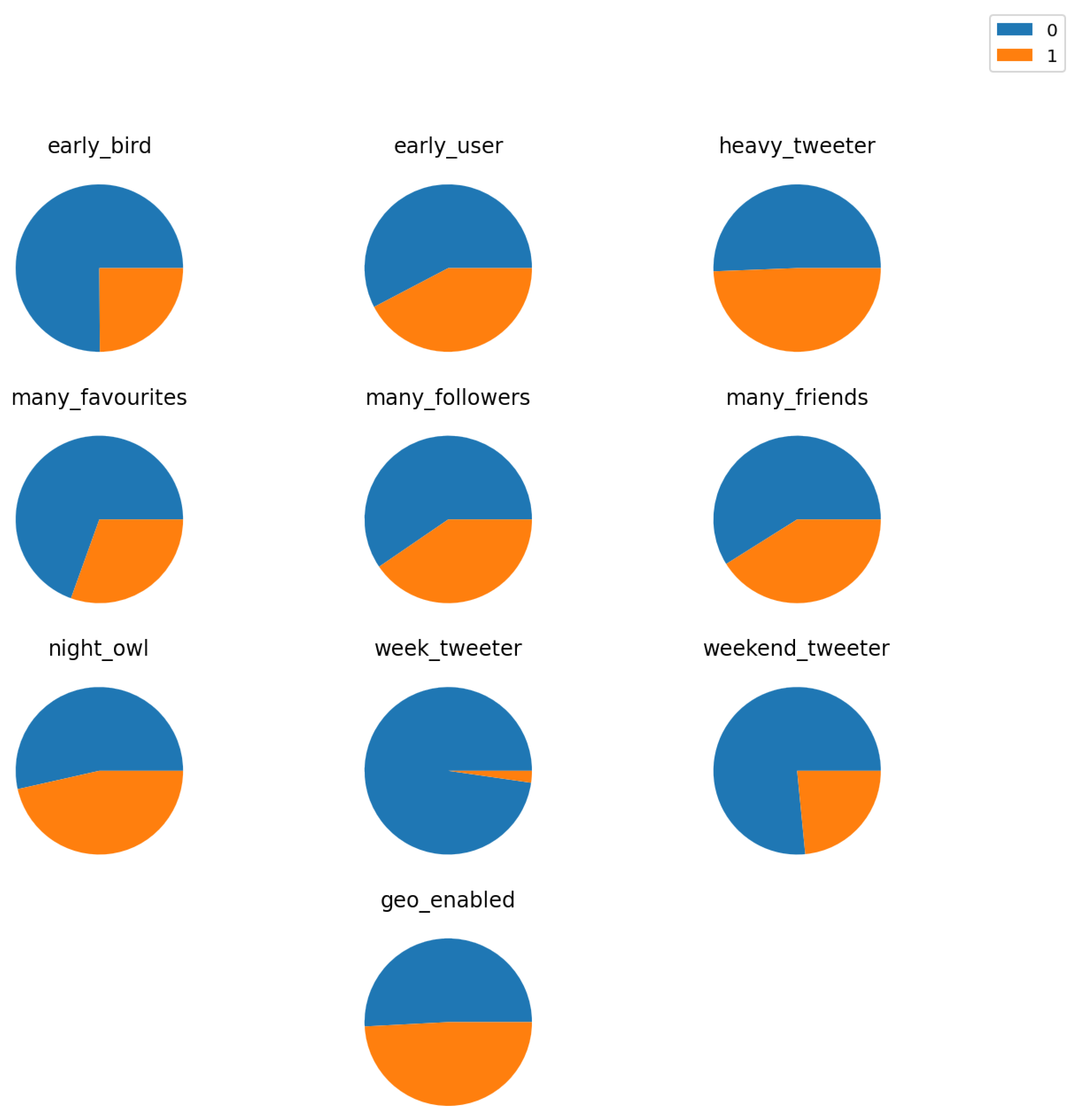
Information 14 00019 g003
Figure 4. All user feature distribution.
Information 14 00019 g004
Figure 5. Rating distribution.
Information 14 00019 g005
Figure 6. Number of rating per user distribution.
Information 14 00019 g006
Figure 7. User rating distribution in comparison with the average of the recommended items (red) and the item rating average from the user (blue).
Information 14 00019 g007
Table 1. Dataframe feature ratings matrix, including the average rating per movie for all different user feature values. The shape of the matrix is (20, 2831), where 20 is the different user feature values, and 2831 is the number of movies after filtering movies without enough ratings.
Movie_id100072100408100958
Feature_keyFeature_value
early_bird06.4639183.9021748.345865
16.5454554.0000008.550000
early_user06.4861113.9571438.401869
16.4827593.8636368.378788
geo_enabled06.3492064.1666678.379310
16.6119403.7000008.406977
heavy_tweeter06.5555564.0000008.218391
16.3965523.8392868.569767
many_favourites06.5217393.8607598.362069
16.3947374.0571438.456140
many_followers06.6296303.8400008.336735
16.2448984.0769238.466667
many_friends06.6000004.0606068.377551
16.3272733.7291678.413333
night_owl06.4705883.7460328.384615
16.5000004.1372558.402439
week_tweeter06.4883723.9115048.390533
16.0000005.0000008.500000
weekend_tweeter06.3958333.9625008.411348
16.7352943.8235298.312500
Table 2. Dataframe movies, including all the movies with all movie features. The shape is (2831, 412), where 2831 is the number of movies, and 412 is the number of features.
ThrillerDramaRomance20 sShortLong
id
100072010000
100408000010
100958000001
Table 3. Dataframe matrix as the result of filtering Table 1 with the features from the user selected. The resulting shape is (10, 2831), where 10 is all the user feature values from selected users, and 2831 is the number of movies.
Movie_id100072100408100958
Feature_keyFeature_value
early_bird06.4639183.9021748.345865
early_user16.4827593.8636368.378788
geo_enabled16.6119403.7000008.406977
heavy_tweeter06.5555564.0000008.218391
many_favourites06.5217393.8607598.362069
many_followers06.6296303.8400008.336735
many_friends06.6000004.0606068.377551
night_owl16.5000004.1372558.402439
week_tweeter06.4883723.9115048.390533
weekend_tweeter16.7352943.8235298.312500
Table 4. Dataframe matrix for affinity showing the ratings from the users with high affinity with the selected user. The shape is (15, 2831), where 15 is the number of users with high affinity and 2831 is the number of movies.
Movie_id100072100408998393999360
User_id
122203NaNNaNNaNNaN
175298NaNNaN0.670.50
204280NaN0.500.831.00
8251861.00NaN0.830.50
8711050.500.500.50NaN
9763460.50NaN1.000.50
Table 5. Array with movie predictions for the selected user according to users with high affinity. The shape is (2831), where 2831 is the number of movies.
Rate
Movie_id
1004080.733333
1009580.666667
1010220.833333
Table 6. Dataframe predictions for a user where the predictions for the selected user are displayed. The shape is (585, 4), where 585 is the number of movies rated by the user from the movie set, and 4 is the number of columns added for predictions.
yyhatyhat_affinityyhat_total
Movie_id
1070607.00.5661040.8875970.726850
1081457.00.6063140.7906980.698506
1092207.00.7127690.8488370.780803
Table 7. Dataframe predictions for the user where the predictions for the selected user are displayed sorted by prediction (highest prediction rank on top). The shape is (585, 4), where 585 is the number of movies rated by the user from the movie set, and 4 is the number of columns added for predictions.
yyhatyhat_affinityyhat_total
Movie_id
74575110.00.9633040.9152820.939293
6552758.00.9176960.9392760.928486
6248279.00.8343510.9983390.916345
4599369.00.9506380.8726890.911664
2526287.00.9261040.8875970.906850
3706399.00.9236770.8765860.900131
Table 8. Results of the recommended item average.
Average Rating of Recommended ItemsAverage Rating from UserImprovement over Average Rating
8.6 (out of 10)7.38 (out of 10)16.53%
Disclaimer/Publisher’s Note: The statements, opinions and data contained in all publications are solely those of the individual author(s) and contributor(s) and not of MDPI and/or the editor(s). MDPI and/or the editor(s) disclaim responsibility for any injury to people or property resulting from any ideas, methods, instructions or products referred to in the content.

