Abstract
The double-inverted pendulum (DIP) constitutes a classical problem in mechanics, whereas the control methods for stabilizing around the equilibrium positions represent the classic standards of control system theory and various control methods in robotics. For instance, it functions as a typical model for the calculation and stability of walking robots. The present study depicts the controlling of a double-inverted pendulum (DIP) on a cart using a fuzzy logic controller (FLC). A linear-quadratic controller (LQR) was used as a benchmark to assess the effectiveness of our method, and the results showed that the proposed FLC can perform significantly better than the LQR under a variety of initial system conditions. This performance is considered very important when the reduction of the peak system output is concerned. The proposed controller equilibration and velocity tracking performance were explored through simulation, and the results obtained point to the validity of the control method.
1. Introduction
Modern control theory flourished during the 1960s, principally due to the development of aerospace dynamics and the emergence of space exploration. Today, automated control systems (ACS) [] are implemented telecommunications, medicine, economics, power and electrical systems, and biology. Emerging trends of mechatronics, specifically robotics, ref. [] exploit these mathematical possibilities. Although robotics and informatics have revolutionized commercial enterprises, the need for better and effective control challenged scientists to develop new mathematical models and concepts such as fuzzy logic, machine learning and neural networks to constrain the system closer to human thinking.
Fuzzy logic is a new theory of mathematics, an extension of classical binary logic [] proposed by the mathematician Lotfi Zadeh in his study of fuzzy sets. Zadeh’s theory was based on a study conducted by Lukasiewicz and Tarski back in the 1920s. The first fuzzy logic controller was developed, manufactured, and integrated into electronic and electrical equipment, such as cameras and washing machines, in Japan in the 1980s [,,,]. The results were rather encouraging and led to further acceptance of the theory. Intelligent navigation systems can now replace human pilots in helicopters with amazing performance [,]. Integrating these controls into difficult and complex systems that previously only humans could operate is very advantageous. Moreover, engineers cooperate with experts to design fuzzy rule-based systems and develop efficient models. In this way, complex processes can be analyzed, and elements closer to human behavior can be found. The descriptor system found in nature is an example of a fuzzy logic controller test case. In this study a double-inverted pendulum on a cart, a classical engineering problem [,,], was used to evaluate a fuzzy logic controller (FLC) compared to a method using a linear-quadratic control (LQR), which will be discussed and analyzed [,,]. The purpose of this paper is to strengthen the arguments in favor of an FLC and to demonstrate its potential and the improvements it can offer to existing control methods for complex physical systems in nature that show chaotic behavior. In that regard, chaotic systems can become more understandable and predictable, while their control can become more efficient with Fuzzy Logic.
2. Double-Inverted Pendulum
2.1. Dip Elements
A DIP is a double pendulum (DP) vertical inversion, a naturally unstable system. It is rather more complicated than a DP, and it is rather difficult to maintain a stable upright position in the event of a disturbance when mounted on an oscillating cart. If the oscillating cart is strictly vertical and of high frequency, the DIP can be stabilized. The system is chaotic because the trajectory of the DIP mass is irregular, and there is no symmetry around the vertical axis y. Figure 1, Figure 2, Figure 3 and Figure 4 illustrate the difference between a single pendulum and a double pendulum.
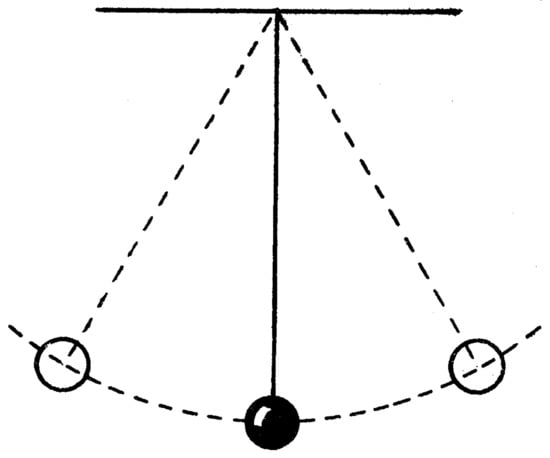
Figure 1.
Single Pendulum [].
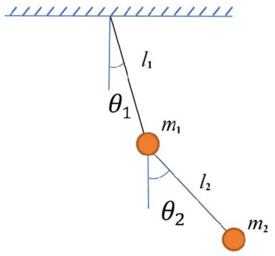
Figure 2.
Double Pendulum [].
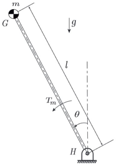
Figure 3.
Inverted Pendulum [].

Figure 4.
Double-Inverted Pendulum [].
A DIP is a system with 3 degrees of freedom (DOFs). The first always moves the cart to the right or left along the x axis. The second DOF is the rotational movement of the first link (link 1) connected to the cart via the revolute joint (joint 1). The third DOF is the rotational motion of the second link (link2), which is connected to the first link via a revolute joint (joint2). The DIP system has the following properties: (i) it is non-linear; (ii) it is multivariable; (iii) it changes rapidly; (iv) it is unstable; (v) it is chaotic (tiny changes have a big effect); and it is among the most challenging problems in automatic control theory. A DIP system can be used as a benchmark to assess the performance of various control methods and has been an exciting research topic over the past years. A DIP model consists of three interconnected bodies: the cart, a first pendulum, and a second pendulum. The dynamics of the system are complex, so we used the Lagrange method for reasons of simplicity.
2.2. Double-Inverted Pendulum Dynamics
The system has three variables: the distance r (or ) that the cart travels along the x axis, the angle of the first link from the positive y axis, and the angle of the second link, again, from the positive y axis. Positive angle values are clockwise and negative angle values are counterclockwise. The horizontal force u on the cart is the sole external force. For the cart, the kinetic energy (), the potential energy () and the dissipation energy () will be [,,]:
where is the mass of the cart, and F is the coefficient of dynamic friction between the cart and the surface. The kinetic energy () of the first pendulum, the potential energy () and the dissipation energy () will be
where is the mass of the first link; is the coefficient of dynamic friction at the first joint; is the moment of inertia of the pendulum; and is the distance between the center of gravity of the first pendulum and the first joint. For the second pendulum, the kinetic energy (), the potential energy () and the dissipation energy () will be
where is the mass of the second link; is the dynamic friction coefficient on the second joint; is the moment of inertia of the second pendulum; and is the distance between the center of gravity of the second pendulum and the second joint. Both pendulums are considered solid bodies of the same density; therefore, both centers of gravity are at their geometric center. Also, the gravitational acceleration value (g) used in all calculations was 9.81 m/s.
2.3. The Lagrange Method
The Lagrange method [,,] calculates the dynamics of the DIP. Subtracting the potential and dissipative energy from the kinetic energy is equivalent to L.
Applying the preceding formula to all three elements of the DIP yields Equations (2) and (3).
where u is the external force applied to the cart, and r is . At this stage, the equations are very complex and software such as MATLAB or Mathematica should be used to solve the symbolic equations, which is why the MATLAB code was built (see []).
2.4. Euler–Lagrange Equations
The Euler–Lagrange equations in matrix form are given in the following: the vector is defined and the vector
consists of three system variables: cart position, first pendulum angle and second pendulum angle as well as their derivatives: cart speed, first pendulum angular velocity, and second pendulum angular velocity as shown in (4).
Therefore, the form of the DIP system is (see []):
where
where:
Since the center of gravity of each pendulum is in its geometrical center, are the lengths of the two links respectively, and the moment of inertia can be calculated as for each pendulum. After some computation, it looks like this:
Therefore, the matrix is symmetrical and non-singular. From (5) we have:
Since the system is non-linear, linearization around the equilibrium point—where the values of the variables are and —should be performed to put the model of the system into its the normal format (14),
to obtain an approximation of the linear solution to the problem of optimal control. The matrices A and B are:
where
This system is ideal, and we can assume that there is no cart movement or friction between the two joints. In this case, ; ; and , so , and the matrix A is simplified to the following format:
2.5. State Space Equations of the Double-Inverted Pendulum
We compute the four A, B, C, and D matrices of the state-space model using the following values: (see Table 1):

Table 1.
The parameter values used for the model.
We can derive a state-space model of the DIP system (see []):
where
and , .
3. Linear Quadratic Regulation Control
The derived model is a Single Input Multiple Output (SIMO) model, and it is unstable. We can study our systems using the controllability and observability matrices, for which MATLAB provides the functions ctrb(sys) and obsv(sys). The controllability matrix is:
and the observability matrix is:
Using MATLAB, the ranks of the Co and Ob matrices can be found, and these are equal to n = 6. Hence, the model is controllable and observable.
The aim of LQR is to compute the appropriate matrix of gains to reach reach the optimal solution for the problem []. The gain of F control must minimize the integral
where and are positive, constant matrices. For infinite time there is
where M satisfies the algebraic Riccati equation and is the solution of
If the system is asymptotically unstable, or if the system defined by A and B is controllable and the system defined by A and E where is observable, there is a unique positive solution M which minimizes the V:
MATLAB uses the LQR command to find a K matrix (gain) for a complete state-feedback of the system. The LQR command has four arguments: the A, B, Q, and R matrices. In the fundamental case, Q and R can be defined as:
The results for the gain matrix K are
Figure 5, shows the open-loop system (grey area) and the closed-loop feedback with the K matrix. The thick lines represent a bus of six signals for the 6 state variables.
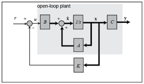
Figure 5.
Block representation of the system with K feedback [].
At this point, one input variable (external force on the cart) and six output variables are used to derive a new closed-loop system. The six output variables are (Figure 6):
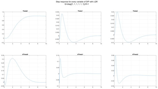
Figure 6.
Step response of the system.
- —Movement of the cart along the x axis
- —Angle of the first pendulum
- —Angle of the second pendulum
- —Velocity of the cart
- —Angular velocity of the first pendulum
- —Angular velocity of the second pendulum
3.1. LQR Customization
In the previous section, LQR was described using the simplest form of the Q and R matrices, yet there are different approaches to choosing those values. References include methods such as Bryson’s Law and many optimization algorithms for Q and R values. The choice to determine the value is up to the engineer and depends on the needs of the problem. For the Q matrix these values are the weights for every state variable, and bigger numbers move the poles of the closed-loop system more to the left in the complex plane. As a result, the system decays to zero more quickly. On the other hand, high R values affect the control effort and slow down the poles. We chose to plot 5 different cases to compare the Q and R values:
Figure 7 Results of the step response of the first three variables in all cases.
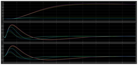
Figure 7.
Step response of all 6 cases (including the initial one). Yellow—Initial simplest form, Blue—1st case (very close to green), Orange—2nd case (very close to purple), Green—3rd case, Purple—4th case, Light Blue—5th case.
The results yielded were similar for the first (yellow), the second (orange) and fourth (purple) cases, whereas the first (blue) and the third (green) cases also had similar results. The fifth case (light blue) results were somewhere in the middle.
3.2. Simulink Model for LQR
We modeled the DIP in a block diagram using the Simulink tools provided by MATLAB. For the LQR method, the Simulink model is in Figure 8.
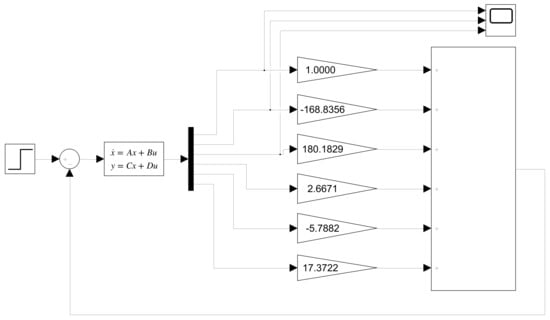
Figure 8.
Simulink model of the LQR control.
The gain value for each state was calculated from the simplest form:
and
as a result
For a step response with amplitude value of 1 and an initial value of 0 degrees for the two pendulums, the cart moves from 0 to 1, whereas the two pendulums after an oscillation stabilize at 0 degrees. After the linearization of the system, the LQR method led to a near-optimal solution to the problem, but left enough space for experimentation on the control of the DIP system.
Given a step response with an amplitude value of 1 and an initial value of 0 degrees for the two pendulums, the cart moves from 0 to 1 and the two pendulums stabilize at 0 degrees after the oscillation. After linearizing the system, the LQR method led to a near-optimal solution, but there was plenty of room for experimentation to control the DIP system.
4. Fuzzy Control
4.1. Fuzzy Logic Controllers
A major advantage of Fuzzy Logic Controllers (FLCs) is that they are quite simple. They consist of three stages: input, process, and output layers []. The sensor signal is tuned at the input layer and is matched to the membership function to provide fuzzy input. At the processing layer, there is a base rule that is triggered in response to an input signal and the result is sent to the output. The output layer is where the fuzzy output is “defuzzified” to a crisp output. Membership functions come in many forms, but the most common are triangular, but they can also be trapezoidal, sigmoidal or Gaussian.
The value of the membership function can be any value in the closed interval [0 1]. The processing layer consists of a rule base and an inference engine. Rules usually take the form
- IF input is A THEN output is B
- IF input1 is A AND input2 is B THEN output is C
The logical operators that could be used are AND, OR, and NOT. The number of basic rules depends on the number of inputs and the number of membership functions for each input. The relationship holds, where m is the number of membership functions and n is the number of inputs. When designing an FLC, sometimes there is a problem called the “explosive growth of rules”. This problem exponentially increases the number of rules in the base, making it very difficult to design an FLC. The inference engine takes the input and produces a fuzzy output according to the rules. There are various FLCs, such as the Mamdani and the Takagi-Sugeno type, that were used in this study depending on the inference engine. The final layer is defuzzification, which produces crisp values as the output of control commands [].
4.2. Fuzzy Logic Controller for the DIP
The FLC Design was created in MATLAB’s Fuzzy Logic Toolbox. The fuzzy system is of the Mamdani type and is based on the results of the LQR method. The shape of the FLC is shown in Figure 9.
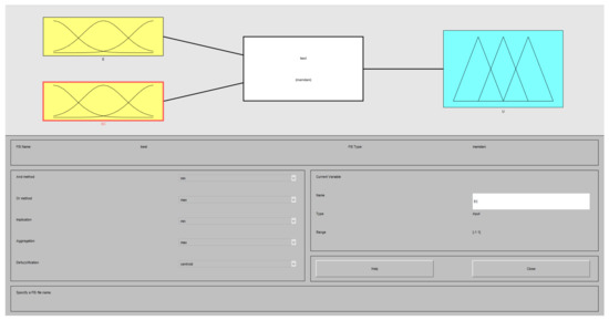
Figure 9.
Form of FLC.
Using all six state variables in the DIP as inputs with three membership functions per variable would require rules, which would cause an explosive problem as stated before. Instead, we used the fusion functions [,] to create two inputs:
- the error e
- the derivative of the error ec
Thus, using the 7 membership functions for each input requires rules. Centroid defuzzification was used because it was the most prevalent and physically appealing of all the defuzzification methods and usually gives superior results [,,,]. The format of the input and output membership functions is shown below in Figure 10.
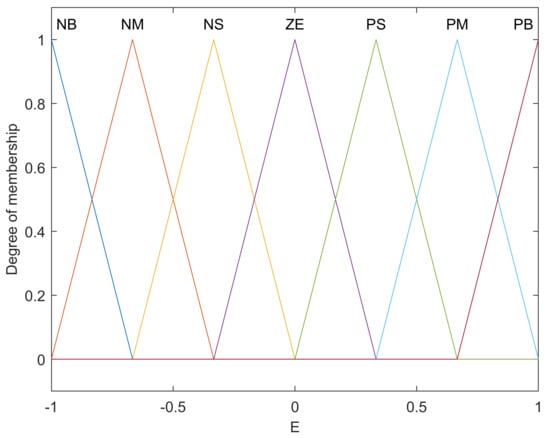
Figure 10.
Inputs e, ec and Output u.
For the rules base, 7 categorical variables were used so that the system behaviour wold be human-like: (i) NB—Negative Big, (ii) NM—Negative Medium, (iii) NS—Negative Small, (iv) ZE—Zero, (v) PS—Positive Small, (vi) PM—Positive Medium, (vii) PB—Positive Big.
These categorical variables match the seven fuzzy sets of the two inputs and outputs. The set of rules is shown in Figure 11.
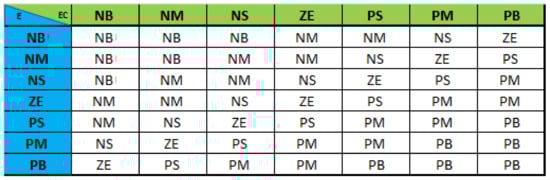
Figure 11.
Rule Base.
An example of a rule is:
- IF E is NB AND EC is NB THEN U is NB
MATLAB’s Fuzzy Logic Toolbox provides RuleViewer, a useful tool that shows which rules are fired for different values. For example, if and then , see Figure 12. Furthermore, in Figure 13, we have the surface plot of the fuzzy system.
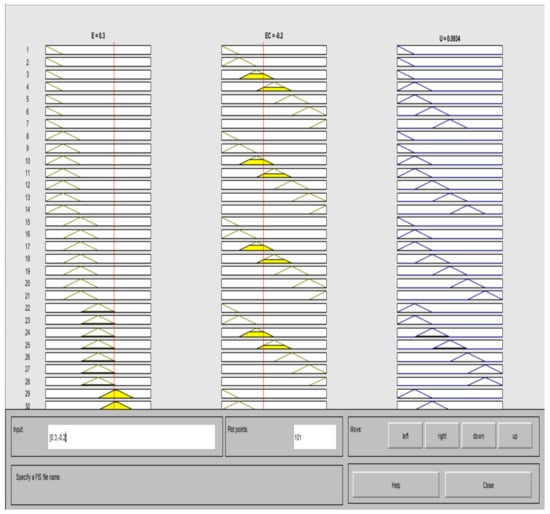
Figure 12.
Rule Viewer.
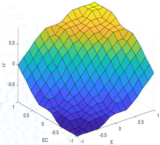
Figure 13.
Surface Graph.
4.3. Creating the Fusion Function
We used fusion functions to implement the FLC models in Simulink. This function had 6 inputs, 6 DIP status variables, and 2 outputs, an error and its derivative. Figure 14 shows the closed-loop system.
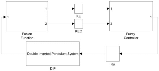
Figure 14.
Closed-loop system.
The output of the DIP is sent to the fusion function, which creates two variables as inputs to the FLC. The three blocks , , and represent the gain of an FLC and were calculated using trial and error to maximize the efficiency of the controller. There are many ways to implement the fusion function, but in this study we chose the upper pendulum angle and its angular velocity as the main variables. We used the following value of K:
The fusion function block diagram in Simulink is shown in Figure 15:
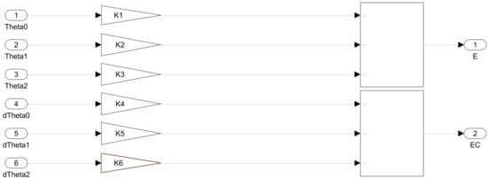
Figure 15.
The fusion function.
The method of calculating the six gains is based on the engineer’s choice according to the parameters in question. The fusion function can be interpreted as weighted sums and the normalization of the input signals. In this study, the focus was the steadiness of the upper pendulum and that led to the division of the first three gains by the second pendulum’s position gain (K3), and the last three with the second pendulum’s angular velocity gain (K6). In that way, the most important elements of the DIP, in our test case, were weighted more as the final input to the FLC inference engine. Hence, the fusion function is
Therefore, 6 state variables can be merged into 2 groups to generate 2 output variables. There are alternative ways to develop the fusion function []. Engineers may set the position and speed of the first pendulum or the position and speed of the cart as the important elements of the problem. It depends on the restrictions of the problem, and further research in this field is mandatory. Another way to create the fusion function is to divide the 6 gains of (29) by the norm of K.
The result is the following fusion function:
4.4. Design of the FLC in Simulink
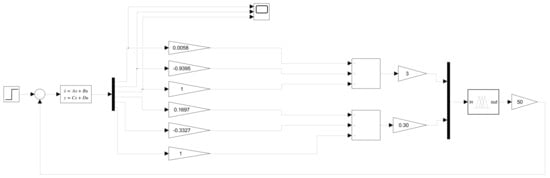
Figure 16.
Simulink blocks of the DIP with the FLC (a).
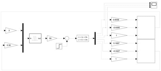
Figure 17.
Simulink blocks of the DIP with the FLC (b).
As a reference signal we used the step function, but the FLC gain value was calculated using trial and error and looked like this:
, , .
Figure 18 shows the results of the first three state variables with a step input and an initial value of zero. The results of the LQR method are also shown here for comparison.
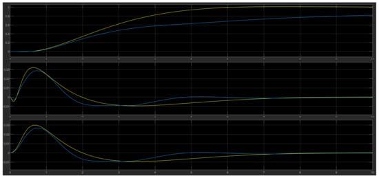
Figure 18.
Comparison of the LQR (yellow) and FLC (light blue) for , and .
As the oscilloscope diagram shows, the FLC controllers had less overshoot and faster settling times than the LQR ones.
4.5. Adjusting the FLC
This section defines another modified FLC that took advantage of different sets of membership functions. After several experiments, we found that the design and intervals of the fuzzy sets had a great influence on the result and the response of the model.
The fix increased the spacing of the membership functions PS, PM, NS, and NM; reduced the ZE interval; and converted the PB and NB triangular functions to Gaussian functions. The new form is shown in Figure 19. The Gaussian membership functions were reported to have shown a smoother response. Input and output ranges were unchanged and in the interval [−1 1]. Moreover, the gain of the new FLC was the same when comparing the result to the first FLC.
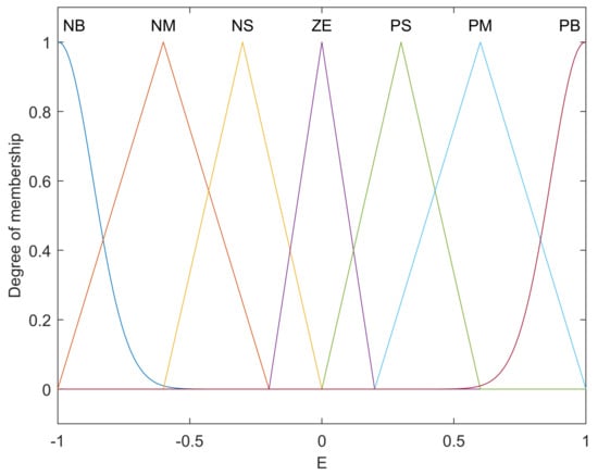
Figure 19.
Inputs/Outputs E, EC and U of the modified FLC.
This new FLC was designed in Simulink, and the experimental results showed that it provided tighter control over the DIP system. Compared to the first FLC, the overshoot ratio was much lower, but the settling time was longer (Figure 20).
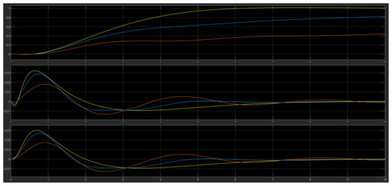
Figure 20.
Comparison of FLC (light blue), LQR (yellow), and the modified FLC (orange).
4.6. Test Results for Various Initial Values of the DIP
So far, we have used an initial value of zero for all calculations, that is, the starting position of the angle for and was at zero degrees (0). What follows is the analysis of the four main cases of initial system values and the measured outputs of all controllers (LQR and two FLCs).
The four typical cases are:
- Both pendulums start at a negative angle, Figure 21 ()
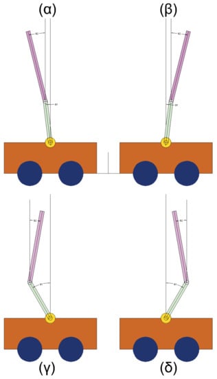 Figure 21. Set of Initial values.
 - Both pendulums start at a positive angle, Figure 21 ()
- The first pendulum starts at a negative angle and the second pendulum starts at a positive angle, Figure 21 ()
- The first pendulum starts at a positive angle and the second pendulum starts at a negative angle, Figure 21 ()
Negative angles go counterclockwise and positive angles go clockwise. The results of the four cases are shown below in Figure 21.
4.6.1. Case 1
For , , the output of the models is in Figure 22.
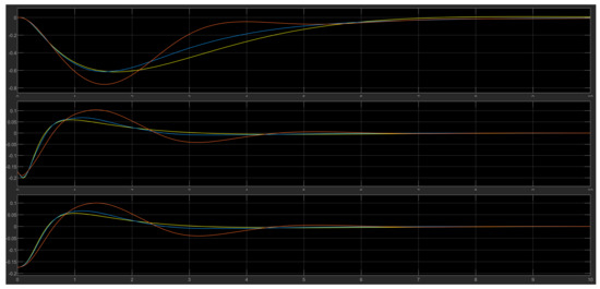
Figure 22.
FLC (light blue), LQR (yellow), and modified FLC (orange).
4.6.2. Case 2
For , , the output of the models is in Figure 23. Cases 3 and 4 are the most difficult to control, but the two FLCs showed considerable efficiency. The modified FLC had a higher overshoot rate than the first FLC.
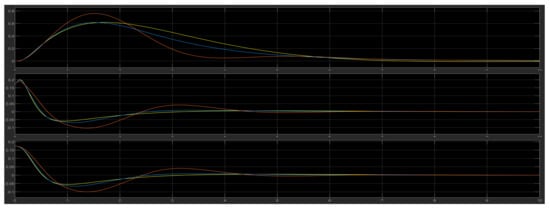
Figure 23.
FLC (light blue), LQR (yellow), and modified FLC (orange).
4.6.3. Case 3
For , , the output of the models is in Figure 24.
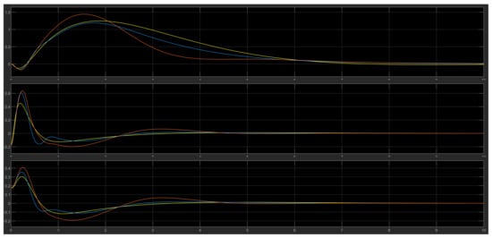
Figure 24.
FLC (light blue), LQR (yellow), and modified FLC (orange).
4.6.4. Case 4
For , , the output of the models is in Figure 25.
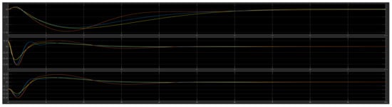
Figure 25.
FLC (light blue), LQR (yellow), and modified FLC (orange).
Finally in Figure 26, the overall representation of all six state variables including the three derivatives (cart speed) (angular velocity of the first pendulum) and (angular velocity of the second pendulum). All three controllers (FLC, LQR, modified FLC) were presented. In these calculations, the reference signal or disturbance from the step source was zero, while the initial values were , . The results show that the two FLCs could stabilize the double-inverted pendulum system. In some cases, better results will be obtained and the LQR method will be improved. The rate of overshoot is small, and the settling time for the DIP to reach a steady state is quite short.
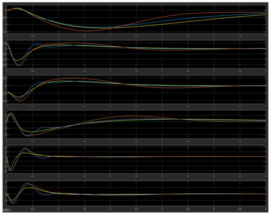
Figure 26.
LQR (yellow), FLC (light blue) and new FLC (orange).
4.7. Disturbance
Regarding the stability of an experimental realistic manufactured DIP system, various repetitive disturbances could be generated due the wind, friction or other external forces in the physical environment.
There were three selected placements for Simulink disturbances: the control signal of the fuzzy controller output; one in each output signal from the plant, and one in the upper pendulum signal (Figure 27). It is obvious that these forces can also be applied to specific components of the DIP system, such as the upper or lower pendulum or even on the cart. The disturbance was implemented with a pulse generator block that created a small amplitude pulse ranging from 0.1 to 1, over a period of 5 s with a 10% pulse width.
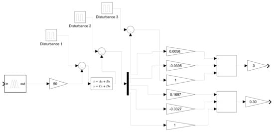
Figure 27.
The external repetitive disturbances in Simulink.
The results of the system’s response with the LQR, FLC and modified FLC controllers for the cart and lower and upper pendulum positions are depicted in Figure 28, Figure 29 and Figure 30 where it is shown that both FLCs had better control over the disturbance and improved overall stabilization of the system with smaller oscillations during the external pulse.
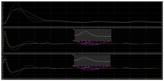
Figure 28.
The DIP response under disturbance (first placement point) in the control signal with the LQR (yellow), FLC (blue) and modified FLC* (orange) controllers.
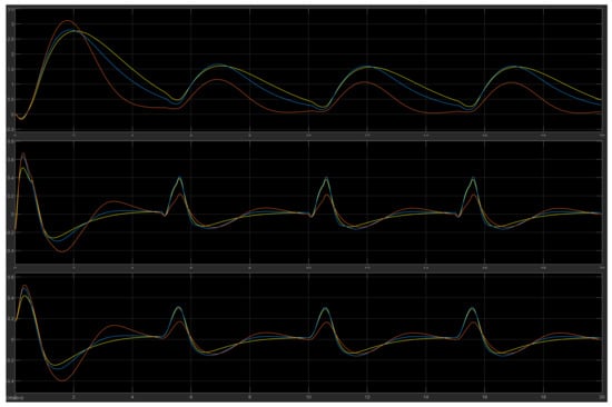
Figure 29.
The DIP response under disturbance (second placement point) in the control signal with the LQR (yellow), FLC (blue) and modified FLC* (orange) controllers.
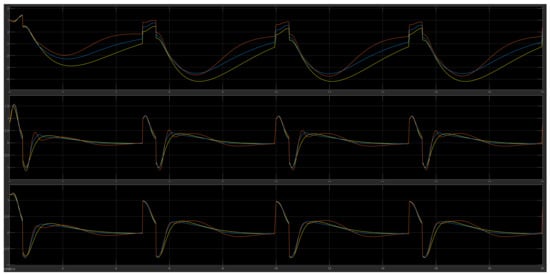
Figure 30.
The DIP response under disturbance (third placement point) in the control signal with the LQR (yellow), FLC (blue) and modified FLC* (orange) controllers.
The system can become more robust with the fuzzy control and solve real-life problems where there are incalculable external factors and energy losses, such as friction, which can result in chaotic behavior. During the disturbance (second placement), the results proved that there was improvement in the overall behavior of the system as depicted in Table 2. The three elemts of both FLCs reached zero faster than the LQR controller did at time 0.1 s before next disturbance occurrence (period of 5 s).
Table 2.
Comparative values under disturbance for all elements at simulation time 4.9 s.
Fuzzy logic can improve and advance existing control theories and methods due to its proximity to the human approach to problem solving. With the capabilities of neural networks, neuro-fuzzy controllers can learn from their operational environment to enhance the potential of control over highly unstable systems.
5. Conclusions
In the present study, the control of a double-inverted pendulum (DIP) on a cart using a fuzzy logic controller (FLC)-based detailed model was proposed in a MATLAB/Simulink environment to test its behavior and achieve good system stability. The simulation results pointed to the efficacy of the FLC in comparison to other widely accepted methods, such as LQR. Although both fuzzy logic and the LQR controller stabilized the system normally, the FLC substantially reduced peak levels as well. An expansion of this controller could be also applied to a triple-inverted pendulum and there are notable efforts in the global bibliography regarding that problem []. All documentation (MATLAB code/Simulink model used was retrieved from []. Suggestions for future research could include expansion of our method using a type 2 fuzzy membership function as well as the Tagaki-Sugeno FLC rather than the Mandani one [,,].
Author Contributions
Conceptualization, G.S.M. and G.F.F.; methodology, G.S.M.; software, G.S.M.; validation, T.L.K. and M.G.T.; writing—original draft preparation, G.S.M.; writing—review and editing, T.L.K., M.G.T. and G.F.F.; supervision, M.G.T. and G.F.F.; funding acquisition, M.G.T. All authors have read and agreed to the published version of the manuscript.
Funding
This research received no external funding.
Institutional Review Board Statement
Not applicable.
Informed Consent Statement
Not applicable.
Data Availability Statement
https://gitfront.io/r/marasgeon/d401cb516187aa5b83beaeab04b15d3885621b56/MATLAB-code/tree/SEEDA/ (accessed on 2 July 2022).
Acknowledgments
Not applicable.
Conflicts of Interest
The authors declare no conflict of interest.
References
- Dorf, R.C.; Bishop, R.H. Modern Control Systems; Pearson: London, UK, 2011. [Google Scholar]
- Craig, J. Introduction to Robotics: Mechanics and Control; Pearson: London, UK, 2018. [Google Scholar]
- Zadeh, L.A. Fuzzy sets. Inf. Control 1965, 8, 338–353. [Google Scholar] [CrossRef]
- Zadeh, L.A. Outline of a new approach to the analysis of complex systems and decision processes. IEEE Trans. Syst. Man Cybern. 1973, SMC-3, 28–44. [Google Scholar] [CrossRef]
- Zadeh, L.A. Fuzzy algorithms. Inf. Control 1968, 12, 94–102. [Google Scholar] [CrossRef]
- King, R.E. Computational Intelligence in Control Engineering; CRC Press: Boca Raton, FL, USA, 1999. [Google Scholar]
- Kosko, B.; Toms, M. Fuzzy Thinking: The New Science of Fuzzy Logic; Hyperion: New York, NY, USA, 1993. [Google Scholar]
- Theodorou, Y. Introduction to Fuzzy Logic (Book in Greek), 1st ed.; Editions TZIOLA: Thessaloniki, Greece, 2010. [Google Scholar]
- Hazem, Z.B.; Fotuhi, M.J.; Bingül, Z. Development of a Fuzzy-LQR and Fuzzy-LQG stability control for a double link rotary inverted pendulum. J. Frankl. Inst. 2020, 357, 10529–10556. [Google Scholar] [CrossRef]
- Hazem, Z.B.; Fotuhi, M.J.; Bingül, Z. A study of anti-swing fuzzy LQR control of a double serial link rotary pendulum. IETE J. Res. 2021, 1–12. [Google Scholar] [CrossRef]
- Fotuhi, M.J.; Hazem, Z.B.; Bingül, Z. Modelling and torque control of an non-linear friction inverted pendulum driven with a rotary series elastic actuator. In Proceedings of the 2019 3rd International Symposium on Multidisciplinary Studies and Innovative Technologies (ISMSIT), Ankara, Turkey, 11–13 October 2019; pp. 1–6. [Google Scholar]
- Luhao, W.; Zhanshi, S. LQR-Fuzzy control for double-inverted pendulum. In Proceedings of the 2010 International Conference on Digital Manufacturing & Automation, Changcha, China, 18–20 December 2010; Volume 1, pp. 900–903. [Google Scholar]
- Kudinov, Y.; Pashchenko, F.; Kelina, A.; Vasutin, D.; Duvanov, E.; Pashchenko, A. Analysis of Control System Models with Conventional LQR and Fuzzy LQR Controller. Procedia Comput. Sci. 2019, 150, 737–742. [Google Scholar] [CrossRef]
- Hazem, Z.B.; Fotuhi, M.J.; Bingül, Z. Anti-swing radial basis neuro-fuzzy linear quadratic regulator control of double link rotary pendulum. Proc. Inst. Mech. Eng. Part I J. Syst. Control Eng. 2022, 236, 531–545. [Google Scholar] [CrossRef]
- The Pendulum. My Attempt at Building a Diverse Company from the Start. Available online: https://medium.com/assist/the-pendulum-my-attempt-at-building-a-diverse-company-from-the-start-bd9e50523a3d (accessed on 1 May 2022).
- Izadgoshasb, I.; Lim, Y.Y.; Tang, L.; Padilla, R.V.; Tang, Z.S.; Sedighi, M. Improving efficiency of piezoelectric based energy harvesting from human motions using double pendulum system. Energy Convers. Manag. 2019, 184, 559–570. [Google Scholar] [CrossRef]
- Bhounsule, P. A Controller Design Framework for Bipedal Robots: Trajectory Optimization and Event-Based Stabilization. Ph.D. Thesis, Cornell University, Ithaca, NY, USA, 2012. [Google Scholar]
- Bogdanov, A. Optimal Control of a Double-Inverted Pendulum on a Cart; Tech. Rep. CSE-04-006; Oregon Health and Science University, OGI School of Science and Engineering: Beaverton, OR, USA, 2004. [Google Scholar]
- Brull, T. Course: Systems and Control Theory; Lecture Notes: Equations of Motion for an Inverted Double Pendulum on a Cart (in Generalized Coordinates); Institute of Mathematics: Berlin, Germany; Available online: https://www3.math.tu-berlin.de/Vorlesungen/SoSe12/Kontrolltheorie/matlab/inverted_pendulum.pdf (accessed on 2 July 2022).
- Jaiwat, P.; Ohtsuka, T. Real-time swing-up of double-inverted pendulum by nonlinear model predictive control. In Proceedings of the 5th International Symposium on Advanced Control of Industrial Processes, Hiroshima, Japan, 28–30 May 2014; pp. 290–295. [Google Scholar]
- Demirci, M. Design of feedback controllers for linear system with applications to control of a double-inverted pendulum. Int. J. Comput. Cogn. 2004, 2, 65–84. [Google Scholar]
- Morin, D. Introduction to Classical Mechanics: With Problems and Solutions; Cambridge University Press: Cambridge, UK, 2008. [Google Scholar]
- Available online: https://gitfront.io/r/marasgeon/d401cb516187aa5b83beaeab04b15d3885621b56/MATLAB-code/tree/SEEDA/ (accessed on 2 July 2022).
- Inverted Pendulum: System Modeling. Available online: https://ctms.engin.umich.edu/CTMS/index.php?example=InvertedPendulum§ion=ControlStateSpace (accessed on 1 May 2022).
- Van Leekwijck, W.; Kerre, E.E. Defuzzification: Criteria and classification. Fuzzy Sets Syst. 1999, 108, 159–178. [Google Scholar] [CrossRef]
- Han, Y.; Liu, Y. Reduced-dimensional fuzzy controller design based on fusion function and application in double-inverted pendulum. In Proceedings of the 2010 The 2nd International Conference on Industrial Mechatronics and Automation, Wuhan, China, 30–31 May 2010; Volume 2, pp. 337–340. [Google Scholar]
- Wang, L.; Zheng, S.; Wang, X.; Fan, L. Fuzzy control of a double-inverted pendulum based on information fusion. In Proceedings of the 2010 International Conference on Intelligent Control and Information Processing, Dalian, China, 13–15 August 2010; pp. 327–331. [Google Scholar]
- Lee, C.C. Fuzzy logic in control systems: Fuzzy logic controller. I. IEEE Trans. Syst. Man Cybern. 1990, 20, 404–418. [Google Scholar] [CrossRef]
- Sugeno, M. An introductory survey of fuzzy control. Inf. Sci. 1985, 36, 59–83. [Google Scholar] [CrossRef]
- Braae, M.; Rutherford, D. Fuzzy relations in a control setting. Kybernetes 1978, 7, 185–188. [Google Scholar] [CrossRef]
- Larkin, L.I. A fuzzy logic controller for aircraft flight control. In Proceedings of the 23rd IEEE Conference on Decision and Control, Las Vegas, NV, USA, 12–14 December 1984; pp. 894–897. [Google Scholar]
- Li, Q.R.; Tao, W.H.; Sun, N.; Zhang, C.Y.; Yao, L.H. Stabilization control of double-inverted pendulum system. In Proceedings of the 2008 3rd International Conference on Innovative Computing Information and Control, Dalian, China, 18–20 June 2008; p. 417. [Google Scholar]
- Hazem, Z.B.; Fotuhi, M.J.; Bingül, Z. A comparative study of the friction models with adaptive coefficients for a rotary triple inverted pendulum. In Proceedings of the 2018 6th International Conference on Control Engineering & Information Technology (CEIT), Istanbul, Turkey, 25–27 October 2018; pp. 1–6. [Google Scholar]
- Elkinany, B.; Alfidi, M.; Chaibi, R.; Chalh, Z. TS fuzzy system controller for stabilizing the double-inverted pendulum. Adv. Fuzzy Syst. 2020, 2020, 8835511. [Google Scholar]
- Chen, W.; Theodomile, N. Simulation of a triple inverted pendulum based on fuzzy control. World J. Eng. Technol. 2016, 4, 267. [Google Scholar] [CrossRef]
- Zhang, C.; Bai, C.; Ding, Y.; Zhang, Q. LQR optimal control of triple inverted pendulum based on fuzzy quotient space theory. In Proceedings of the 2012 IEEE International Conference on Granular Computing, Hangzhou, China, 11–13 August 2012; pp. 633–638. [Google Scholar]
Publisher’s Note: MDPI stays neutral with regard to jurisdictional claims in published maps and institutional affiliations. |
© 2022 by the authors. Licensee MDPI, Basel, Switzerland. This article is an open access article distributed under the terms and conditions of the Creative Commons Attribution (CC BY) license (https://creativecommons.org/licenses/by/4.0/).