An Improved Complete Coverage Path Planning Method for Intelligent Agricultural Machinery Based on Backtracking Method

Abstract

The advancement of society and technology has promoted the development of modern agriculture. It has become a trend to replace traditional manpower with intelligent agricultural machinery that operates independently. As the core technology of intelligent agricultural machinery, complete coverage path planning technology has become more important. At present, the complete coverage path planning algorithms still suffer from problems such as sacrificing the coverage rate to obtain the minimum energy consumption, taking a long time to calculate the algorithm, and destroying crops across the covered region. In view of the above problems, an improved complete coverage path planning algorithms based on backtracking is proposed combined with the actual needs of intelligent agricultural machinery for planting seedlings to improve four aspects: repeated coverage, search efficiency, path planning, and sub-regional crossing. Firstly, the Morse decomposition method is used to divide a complex farmland region into simple sub-regions. Then an improved backtracking method based on a greedy algorithm is proposed in order to reduce the computational efficiency of the current region connection algorithms. The priority principle and the strategy of moving along the boundary are used to solve the problems of region crossing and sacrificing the coverage rate, thereby improving the performance of the current complete coverage path planning method. Compared with the traditional backtracking method, the experimental results show that the number of backtracking points is decreased by about 70% and the occurrence of crossing sub-regions has been significantly reduced. This proposed method can improve the coverage and operating efficiency of intelligent agricultural machinery operations and provide technical support for agricultural operations such as sowing, tillage, and harvesting, thus improving the quality and efficiency of agricultural production.

1. Introduction

1.1. Research Advances of Complete Coverage Path Planning

Agriculture plays a strategic role in the economic development of a country. With the aging of the population and the increase in urban population, the phenomenon of labor shortages in agricultural production is becoming more and more obvious [1]. In order to avoid agricultural production relying on manpower, the United States, Germany, and Japan have successively proposed intelligent agriculture development strategies to greatly increase agricultural labor productivity, land output, and the utilization of resources. Intelligent agricultural machinery (IAM) [2,3,4] is an important part of intelligent agriculture and an important means to improve the quality and benefits of agricultural development [5,6,7]. Complete coverage path planning (CCPP) technology is one of the core technologies of IAM.

CCPP aims to achieve a complete traversal of the map of an entire work region based on the known environment [8,9]. At present, there are two common methods for complete coverage path planning: random CCPP, hybrid CCPP [10]. The advantages of random CCPP are simple and easy to implementation. But there are also disadvantages such as the randomness of the running trajectory, the high repetition rate, and the inability to cover the entire region. Therefore, researchers have mainly studied hybrid CCPP algorithms. In 2009, Timo et al., proposed top-down and bottom-up search methods combined with a greedy algorithm to achieve CCPP for agricultural machinery [11]. In 2014, Deng et al., proposed an improved back propagation neural network local path planning algorithm based on the grid method, which is based on the idea of priority traversal to realize CCPP for a lawn-mower robot [12]. In 2017, Khan et al., proposed an optimized backtracking mechanism for online cattle farming combined with a two-way proximity search algorithm based on unknown areas to achieve CCPP [13]. Hong et al., proposed a heuristic template combined with a backtracking mechanism of greedy criteria to achieve CCPP [14]. Xu et al., proposed two methods to achieve CCPP for farmland areas [15]. He proposed a path planning method for a single operation area using boustrophedon cellular decomposition algorithm combined with the Reeb graph and Euler circuit. In 2018, Ma et al., proposed CCPP for high-precision grid positioning and low-resolution grids combined with biologically inspired networks. The disadvantages of this algorithm were the increase in time and repetition rate [9]. Wang proposed a dual heuristic optimization algorithm combining the ant colony algorithm with the taboo search to achieve CCPP [16]. Nakamura et al., proposed a path planning algorithm to reduce the number of cells a robot must pass through to achieve CCPP for a sweeping robot [17]. Cao et al., proposed an algorithm based on the grid reliability function for dynamic obstacle avoidance to effectively realize the CCPP for a robot, but it has not been verified in an real work environment [18]. Jian et al., proposed a CCPP based on the grid reliability function combined with back-and-forth path planning [19]. Liu et al., proposed avoiding obstacles based on their radius and the relative position to achieve CCPP for agricultural machinery [20]. In 2019, Li et al., proposed the West-Move First algorithm combined with the backtracking method to achieve CCPP, but for complex environments, coverage efficiency is reduced and time complexity is increased [21]. Chen et al., proposed the high efficiency template method, integrating the dynamic window method to realize the CCPP of a service robot [22]. Its disadvantage is that the repeated coverage rate of the algorithm increases. In 2020, Wang proposed the biologically inspired neural network algorithm combined with a depth-first search (DFS) to achieve CCPP for mining robots [23]. Zhou et al., proposed a biologically stimulated neural network algorithm based on the boustrophedon cell decomposition method to perform area traversal to achieve CCPP for mining robots [24]. In the field of actual agricultural production, John Deere, a famous agricultural machinery enterprise, has developed a kind of agricultural machinery intelligent planning software named AutoTrac. This software mainly provides operation support for agricultural machinery drivers based on satellite positioning. But it does not have the function of automatic planning for automated unmanned agricultural machines.

1.2. Brief Analysis of the CCPP Research

The above algorithms provide different ideas for the research into CCPP and promote the development of CCPP technology. However, the CCPP for mobile robots generally sacrifices the repetition rate to obtain the minimum energy consumption. In addition, for the operation of IAM like rice transplanting machinery, it needs to avoid repeated coverage and avoid crossing sub-regions of the active farmland in order to ensure the quality of work.

Therefore, focusing on the problems of current CCPP methods, a novel CCPP algorithm based on an improved backtracking method is proposed. The idea of the algorithm is as follows. The Morse decomposition algorithm combined with the improved backtracking method is used to realize the CCPP of the farmland area by intelligent agricultural machinery, including regional decomposition, CCPP in sub-regions, and regional connection. Regional decomposition involves the division of the farmland region through the Morse decomposition algorithm. Thus, the farmland region with obstacles will be divided into a series of simple and barrier-free sub-regions. The CCPP in a single sub-region aims to achieve a complete traversal of the simple round-trip traversal method. The regional connection uses an improved backtracking method combined with priority rules to achieve the sequence of traversal between regions. The algorithm proposed in this paper can improve the coverage rate, reduce the repeated coverage rate and crossing sub-regions during the operation of IAM, and improve the search efficiency.

The rest of the paper is organized as follows. Section 2 introduces the technologies related to the CCPP algorithm. Section 3 describes the design and implementation of the improved CCPP algorithm based on the backtracking method. The experiments and analysis of the algorithm are given in Section 4. Section 5 concludes the paper and points out some future works.

2. Related Technology

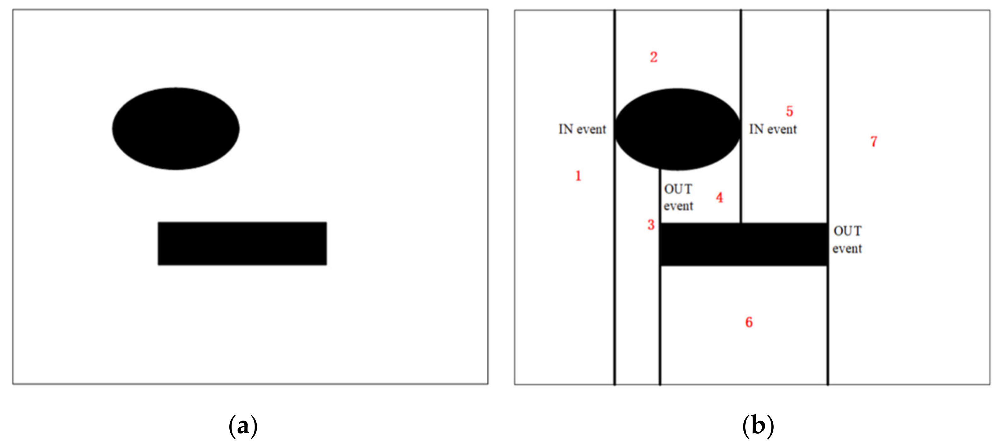
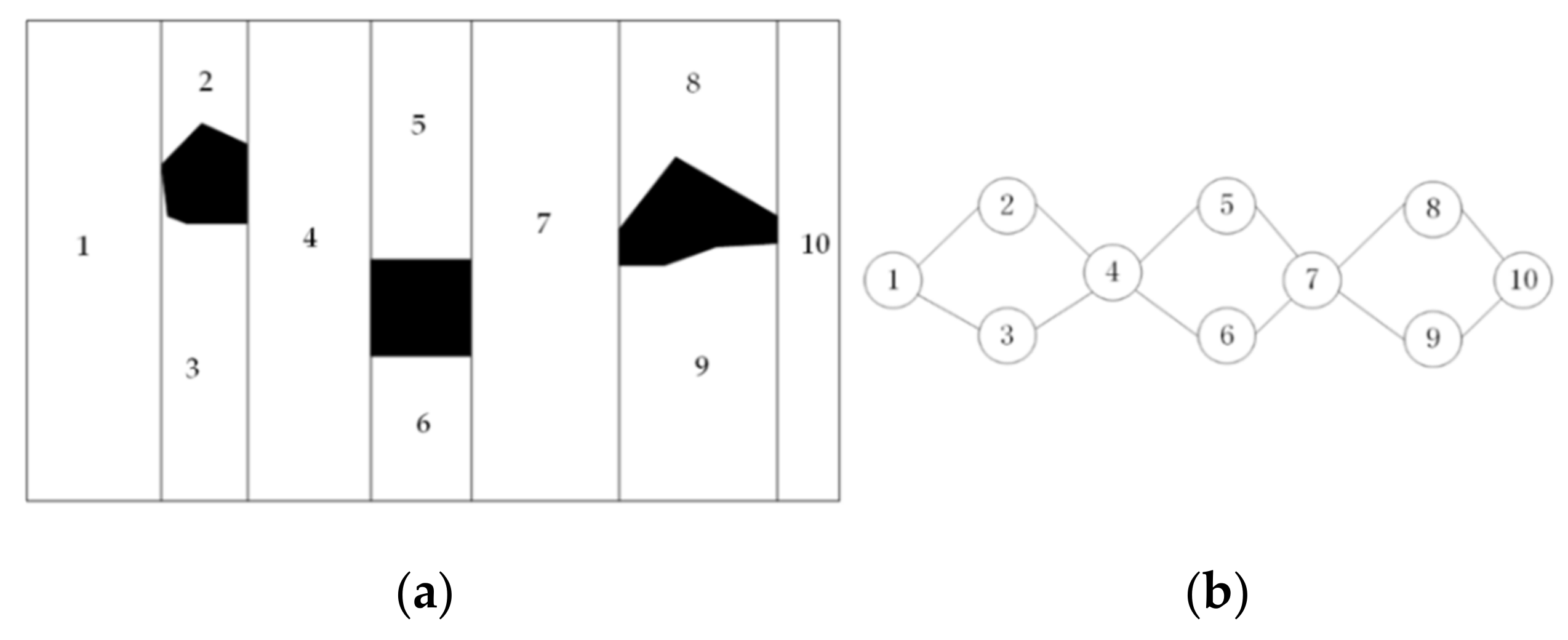
2.1. Morse Decomposition Method

The cell decomposition method includes the trapezoidal [25], boustrophedon [26], and Morse [27,28] decomposition methods, among others. In order to solve the problem of too many sub-cells generated by the trapezoidal decomposition method, the work in [29] proposed the boustrophedon decomposition method, but the premise of this method is to assume that the obstacle is a polygon. The work in [30] points out that the obstacles in Morse decomposition can be of any shape. In this paper, the Morse decomposition method is used to divide the farmland map. The Morse decomposition method divides the farmland map according to a critical point, which is the local extreme value or inflection point. According to the actual needs of the farmland, the optimal decomposition plan is obtained by constructing different Morse functions. Compared with other methods, the Morse decomposition method reduces the number of sub-regions. Thus, the Morse decomposition method is used as the division method for complex regions.

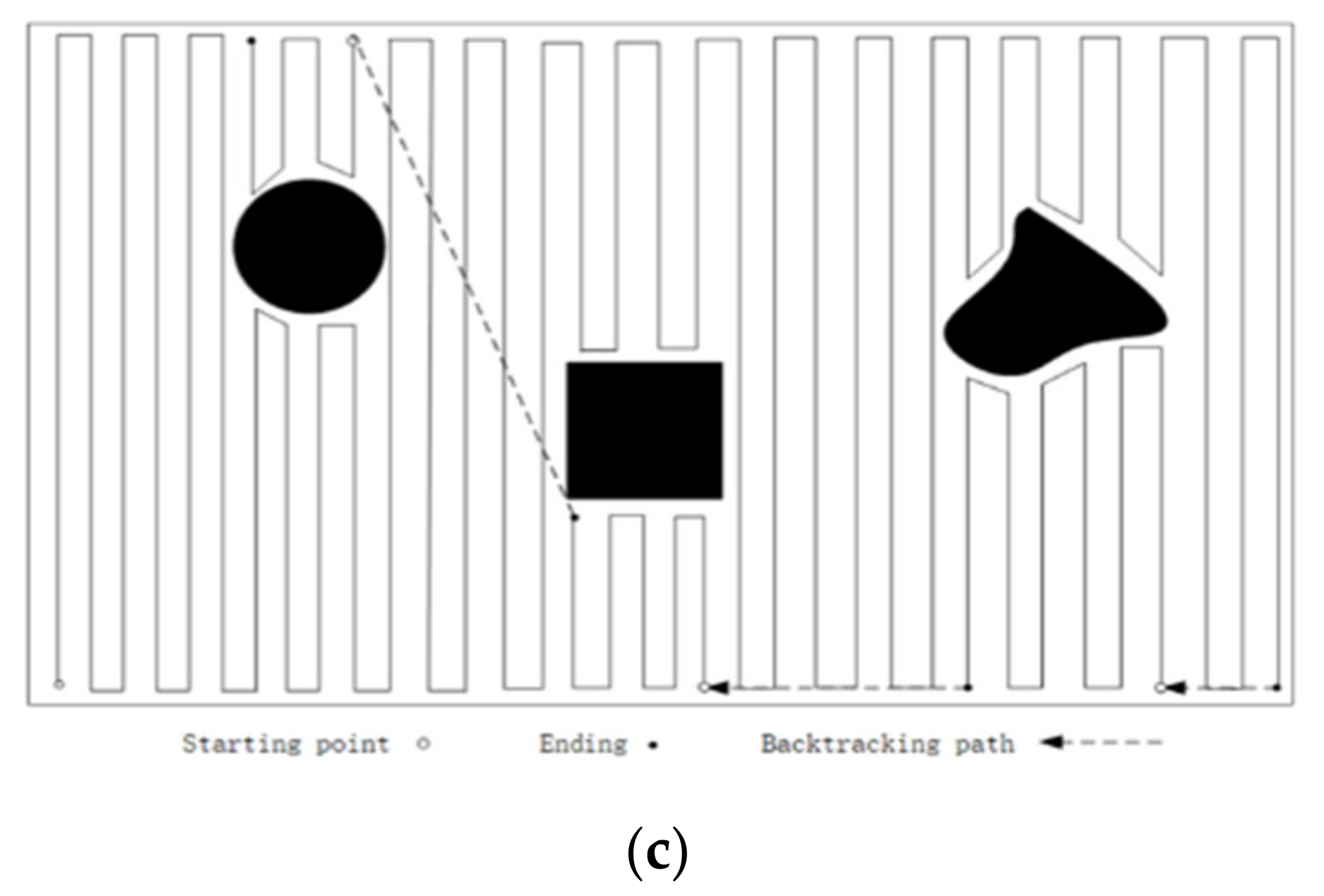
2.2. Backtracking Method

The traditional backtracking method mainly uses the depth-first traversal algorithm combined with connected graphs to achieve CCPP. The connected graph generated from Figure 1a is shown in Figure 1b, where the traversal sequence obtained by DFS is $1\to 3\to 4\to 5\to 7\to 8\to 10\to 9\to 6\to 2$, and the CCPP obtained is shown in Figure 1c.

The backtracking mechanism includes three parts: establishing a list of backtracking points, filtering backtracking points, and selecting backtracking points. Since the traditional backtracking method may lead to an increase in repetition rate, inefficient processing of complex regions, and crossing sub-regions, an improved backtracking method based on the actual situation of farmland areas is proposed and a complete backtracking mechanism is established to ensure that IAM moves along the boundary, which improves the working efficiency of the machinery.

3. Complete Coverage Path Planning with Improved Backtracking Method

Focusing on the problems of the robot CCPP method in the operation of IAM, the research concerning CCPP based on three aspects: regional decomposition, CCPP in sub-regions, and sub-region connection.

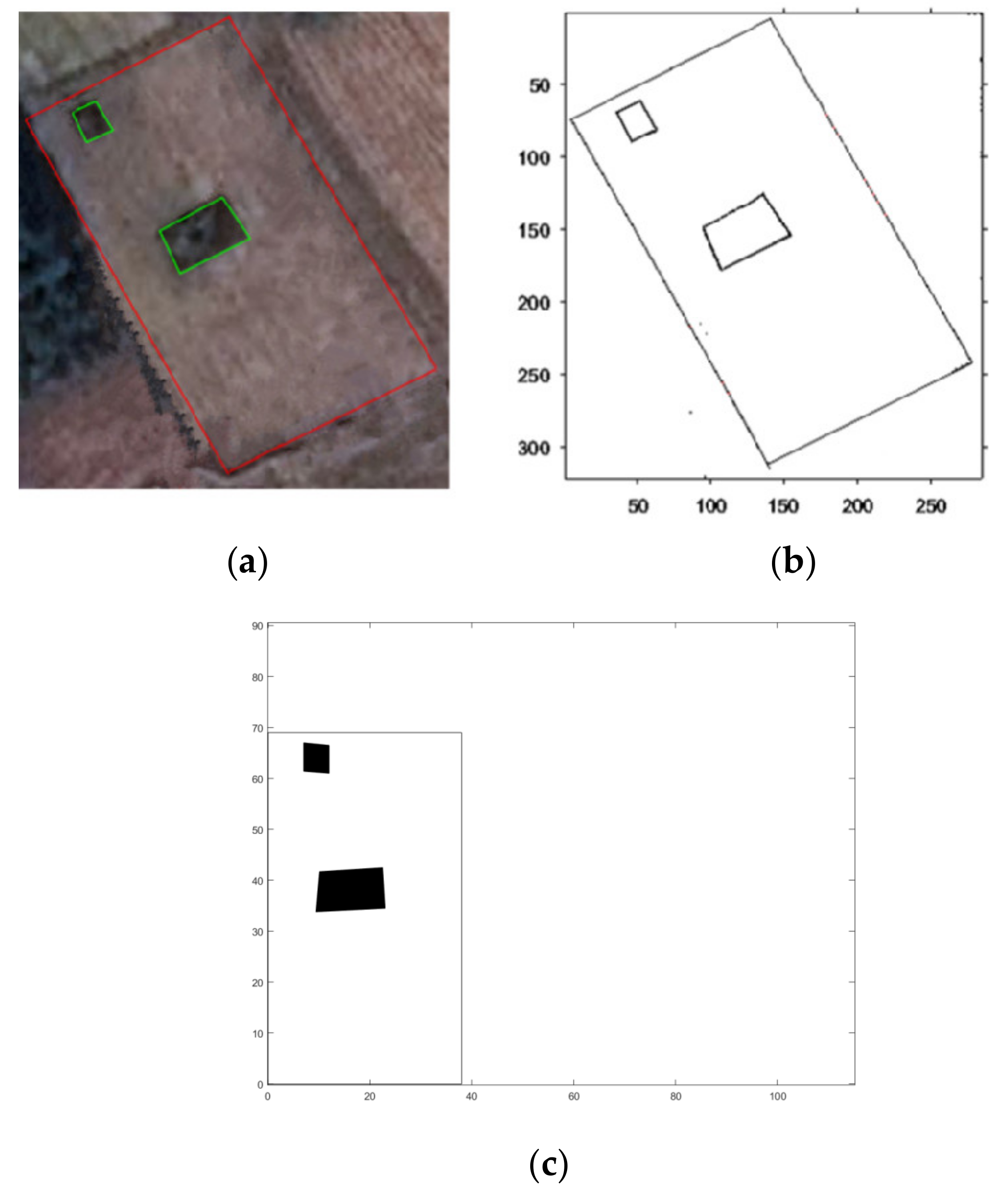
3.1. Regional Decomposition Strategy Based on Morse Theory

At present, CCPP based on the regional decomposition strategy has become the focus of research. The decomposition of regions should refer to the following rules. The decomposition should be carried out along the walking direction of IAM as far as possible, and the sub-region should be divided by the boundary of regions and the boundary of obstacles. Through the above rules, the decomposition times can be reduced, which is convenient for the operation of IAM. When there are many obstacles in the farmland area, IAM cannot complete work smoothly due to the appearance of obstacles and the resulting repeated or missing coverage. The regional decomposition strategy in this paper divides the sub-regions according to the obstacles in the farmland area. Therefore, the whole farmland area is divided into several simple sub-regions, which improves the operation efficiency of IAM.

Based on a two-dimensional plane, the Morse function $f\left(x,y\right)=x$ is used. The Morse decomposition method introduces the process and implementation of the algorithm in detail in Algorithm 1.

Algorithm 1: Procedure for Morse decomposition

BEGIN

Input: farmlandmap.jpg

Image = mpimg.imread (‘ farmlandmap.jpg’)

H,W = image.shape     //Length and width of map

binary_image = (image > 127) //Binarization

Connectivity = 0      //Connectivity

connectivity_parts = []

For x in range(binary_image.shape [1]) do

current_slice ← binary_image[:, x]

connectivity, connective_parts ← calculate_connectivity(current_slice) //Return

connectivity and the number of connected regions

END For

For i in range(last_connectivity) do

IF np.sum(adjacency_matrix[i, :]) > 1 THEN //In event

For j in range(connectivity) do

IF adjacency_matrix[i, j] THEN

total_cells_number ← total_cells_number + 1

current_cells[j] ← total_cells_number

END IF

END For

ND IF

END For

For j in range(connectivity) do

IF np.sum(adjacency_matrix[:, j]) > 1 THEN    //Out event

total_cells_number ← total_cells_number + 1

current_cells[j] ←total_cells_number

ELSEIF np.sum(adjacency_matrix[:, j]) = 0 THEN //In event

total_cells_number ← total_cells_number + 1

current_cells[j] ← total_cells_number

END IF

last_connectivity ← connectivity

last_cells ← current_cells

END For

pickle.dump([decomposed, total_cells_number, cells], open(ccpp_test +”/decomposed_result”, “wb”)) //Save partition file

decomposed_image = np.zeros([H, W, 3], dtype = np.uint8) //Show split result

decomposed_image[decomposed > 0, :] = [255, 255, 255]

Output: decomposition_farmlandmap.jpg

END Morse decomposition

The Morse decomposition method is used to divide the area in Figure 2a, and the result of the division is shown in Figure 2b. The in-event indicates that the current region is terminated and a new region is generated. The out-event indicates that multiple sub-regions are merged into one region.

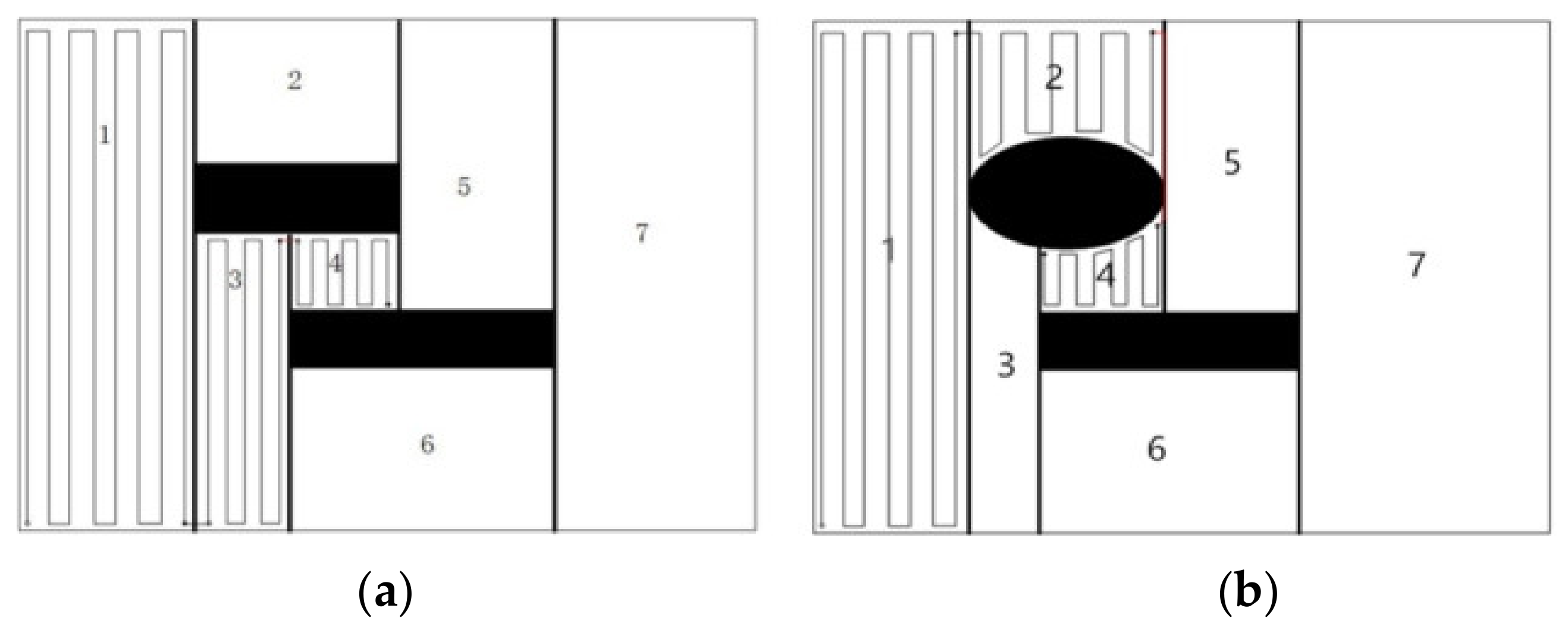
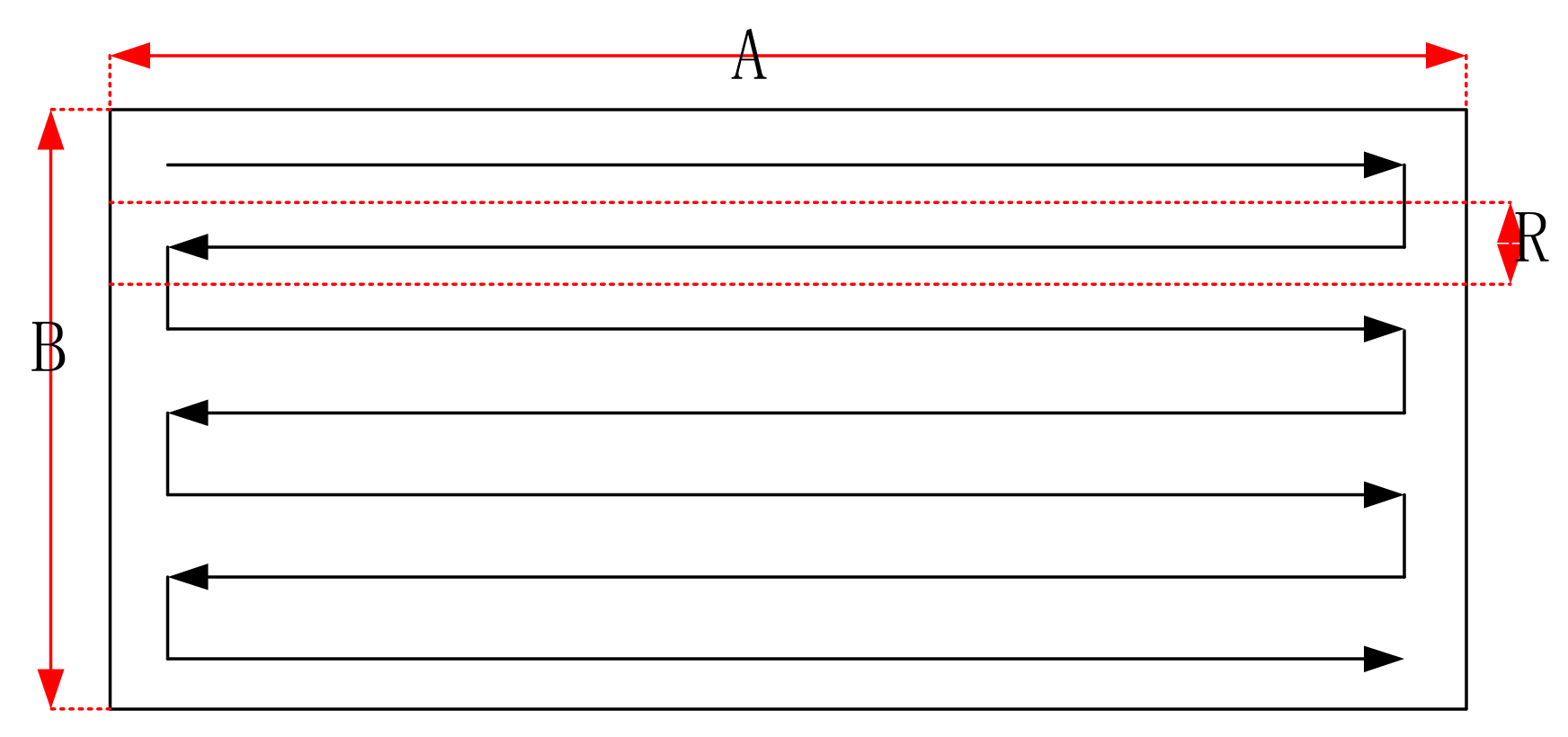
3.2. Complete Coverage Path Planning Method in Sub-Region

After the Morse decomposition method has been used to divide the area into simple sub-regions, round-trip path planning is used to traverse sub-regions. It is necessary to determine the movement direction of the IAM. If the movement direction is changed, the number of turns and the moving distance of the IAM will vary. The trajectory of the movement is related to the energy and time consumed to cover the entire area.

The total energy consumption E_S expression of IAM in the process of linear movement is:

$$E_{S}S=F_{S}S=\frac{F_{S}M}{R}$$

(1)

$F_S$ represents the force required for an IAM to move, and $S$ represents the total distance of linear movement. R represents the robot diameter, and $M$ represents the area of the region.

The total energy consumption $E_T$ of IAM turning is:

$$E_T=E_{0}N={\frac{E_{0}L}{R}}_{}$$

(2)

The energy consumption of each turn of an IAM is set to $E_0$. N is the total number of turns. L is the length in the turning direction.

In summary, the total energy consumption E of an IAM is:

$$E=E_S+E_T= \frac{F_{S}M}{R}+\frac{E_{0}L}{R}$$

(3)

$F_S$, $E_0$, $M$ and R are all fixed values. Thus, the main factor affecting $E$ is $L$.

If $E$ is small, $L$ must also be small. As shown in Figure 3, $L_{begin}$ is:

$$L_{begin}=max\left\{A,B\right\}=A$$

(4)

Therefore, the strategy of move along the long side of the region is chosen and the round-trip traversal rule is used to completely cover simple sub-regions.

3.3. Sub-Region Connection Strategy

Based on the Morse decomposition method, the farmland area is divided into several sub-regions. After combining round-trip path planning to achieve partial coverage of the current sub-region, this work considered how to achieve regional connection and solve the following three problems in the process of regional connection: the problem of IAM crossing sub-regions during the connection process, reducing the problem of repeated coverage, and achieving as far as possible the lowest energy consumption for the connection between sub-regions. In response to the above problems, a backtracking mechanism based on priority rules is established combined with the strategy of moving along the boundary to achieve CCPP.

3.3.1. Create a Backtracking List

The backtracking point list is mainly used to store backtracking points, including recording uncovered regions to find the shortest regional connection target point. The traditional backtracking list records all the uncovered environmental information in the partial traversal. The improved backtracking list in this paper takes into account the environmental information accumulated in the local traversal process of IAM and records the information relating to intersections with obstacles and regional boundaries during the area division process.

There are two principles to follow when building backtracking lists.

Principle 1: The backtracking list only stores the vertex information generated by the intersection with obstacles and boundaries.

Principle 2: The distance between the backtracking point and the end point of the previous region should be as small as possible.

Principle 1 reduces the number of backtracking points and shortens the calculation time. Principle 2 can reduce the length of the movement path between sub-regions and reduce energy consumption. Through the above two principles, the length of the backtracking list can be reduced.

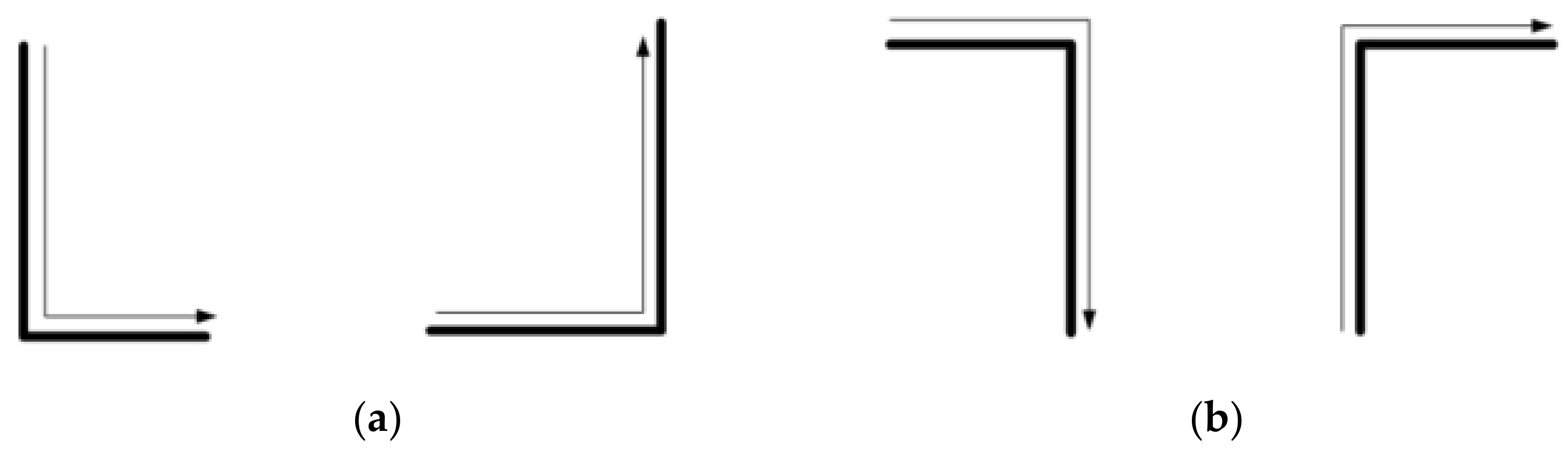
3.3.2. Backtracking Point Selection Principle

Based on the actual consideration of the IAM, in order to further improve the performance of the algorithm, a list of backtracking points is established, the connection to the region based on the priority criterion is realized, and the local optimal backtracking point in the current state from the backtracking list is selected by combining the greedy algorithm strategy and the distance formula.

In this paper, the greedy algorithm is combined with the Manhattan distance formula. Each backtracking considers the backtracking point with the closest distance from the current point to the starting point of the next region and the formula is as follows:

$$n_s=\underset{n\in l_{back}}{\arg }min(d \left(n_{t,} n\right))$$

(5)

In the formula,$n_t$ indicates the end point of the region, $n_s$ indicates the point of the backtracking list selected in the current state, $l_{back}$ represents a backtracking list, $d\left(n_t,n\right)$ represents the Manhattan distance of the current node from elements in the backtracking list as shown in Formula (6). The priority principles are as follows.

$$d\left(n_t,n\right)=\left|n_{ts}-x\left|+\right|n_{ty}-y\right|$$

(6)

Principle 1. Priority of intermediate regions.

Combined with the actual situation of the farmland area, the IAM first traverses the border region adjacent to an intermediate region and finally traverses the intermediate region. During the process of traversing the intermediate region, the machine passes through the traversed region again, and the second traversal occurs. Since the second traversal will destroy the plants in the farmland, it does not meet the needs of agronomy. In order to solve this problem, the principle of priority in intermediate regions is proposed, which makes the IAM in the intermediate region first during the traversal process. Firstly, this work considers whether the current region is an intermediate region. If the adjacent region of the current region or the region with the same $max\_x$ value as the current region belongs to the intermediate region, this region will be traversed first.

Principle 2. Priority of adjacent regions.

If it has been judged in the work environment that principle 1 is not satisfied, there are no intermediate regions or the intermediate regions have been traversed. Then the adjacent region will be given priority. The judgment principle of the adjacent region has the following two situations:

$$curren{t}_x+robo{t}_{radius}=cell.min\_x$$

(7a)

$$curren{t}_x-robo{t}_{radius}=cell.max\_x$$

(7b)

Case 1: The adjacent region is to the right of the last traversed region, as shown in Figure 4a: region 4 has been traversed, and it is judged that the adjacent region meets Formula (7a). The x-value of the starting point of the next region (the minimum value in the regions) is the sum of the x-coordinate of the current point and the radius value of the robot, and the adjacent region is obtained as region 5. The next movement region is region 5.

Case 2: The adjacent region is to the right of the last traversed region, as shown in Figure 4b. Region 4 has been traversed, and it is judged that the adjacent region meets Formula (7b), and the adjacent region is obtained as region 3. Then the next movement region is region 3.

Principle 3. The principle of moving along the boundary.

Since the IAM cannot traverse regions of farmland, the coordinate size of the starting point of the nearest region and the end point of the previous region is first determined in the process of region connection. If the coordinates of the two points are not equal, it is preferred to move along the boundary of the nearest region to the starting point of the next region. The turning situation that the IAM may encounter when moving along the boundary is shown in Figure 5. When the IAM reaches the boundary region of the farmland, that is, $current\_x-robot\_radius=cell.min\_x$ or $current\_x+robot\_radius=cell.max\_x$, the IAM moves along the inner boundary, as shown in Figure 5a. When the IAM moves to the non-boundary region of the farmland, that is, $current\_x-robot\_radius\ne cell.max\_x$ and $current\_x+robot\_radius\ne cell.max\_x$, it moves along the outside boundary, as shown in Figure 5b.

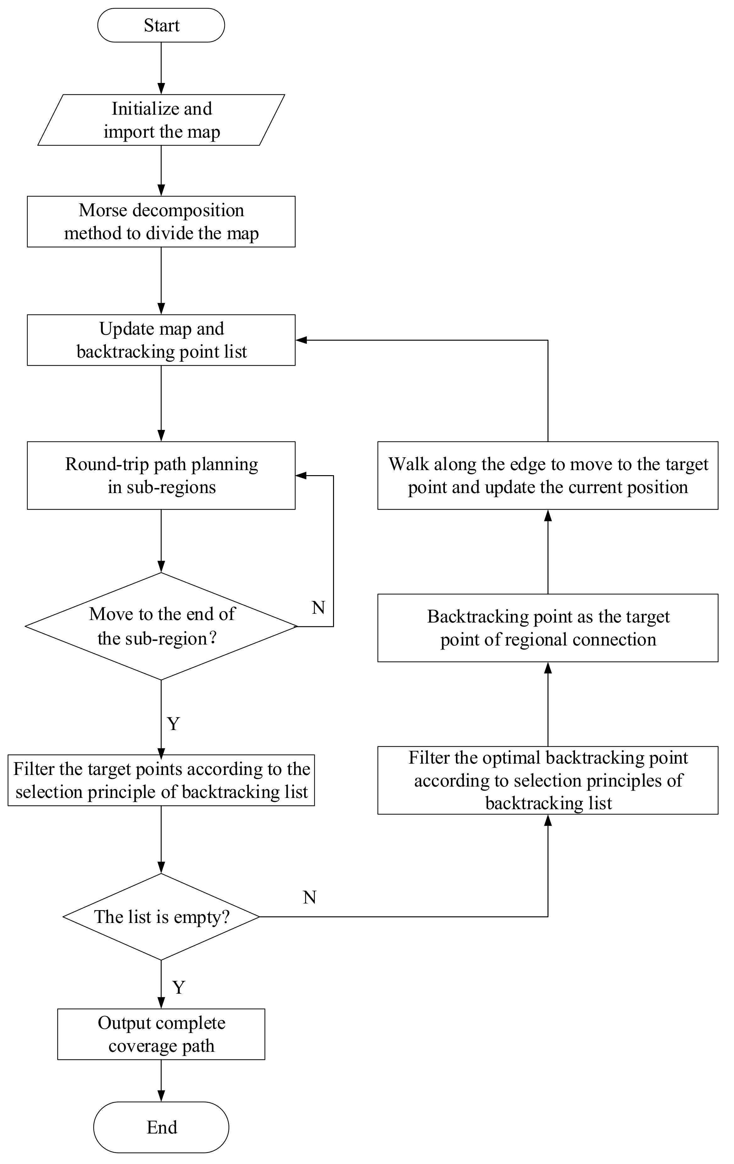
3.4. Method Integration

Combined the above two strategies and one method, an improved CCPP based on the backtracking method is constructed. The flowchart is shown in Figure 6.

When the IAM uses the improved CCPP algorithm proposed in this paper to plan a complete coverage path for the workspace, it is necessary to input the farmland map into the IAM. In the next step, the IAM uses the Morse decomposition method to segment the farmland map and stores the backtracking point information during the segmentation process to establish a backtracking list. Then, it combines the round-trip path planning method to partially cover the current sub-region. After the current sub-region is completely covered, a better backtracking point is selected according to the priority and selection principles for the backtracking points. Then, according to the distance formula combined with the strategy of moving along the boundary, the shortest path from the end of the previous region to the start of the next region is found. The above steps are repeated until the backtracking list is empty. Then the complete coverage path is output, and full coverage of the entire workspace will be achieved.

4. Experiment and Analysis

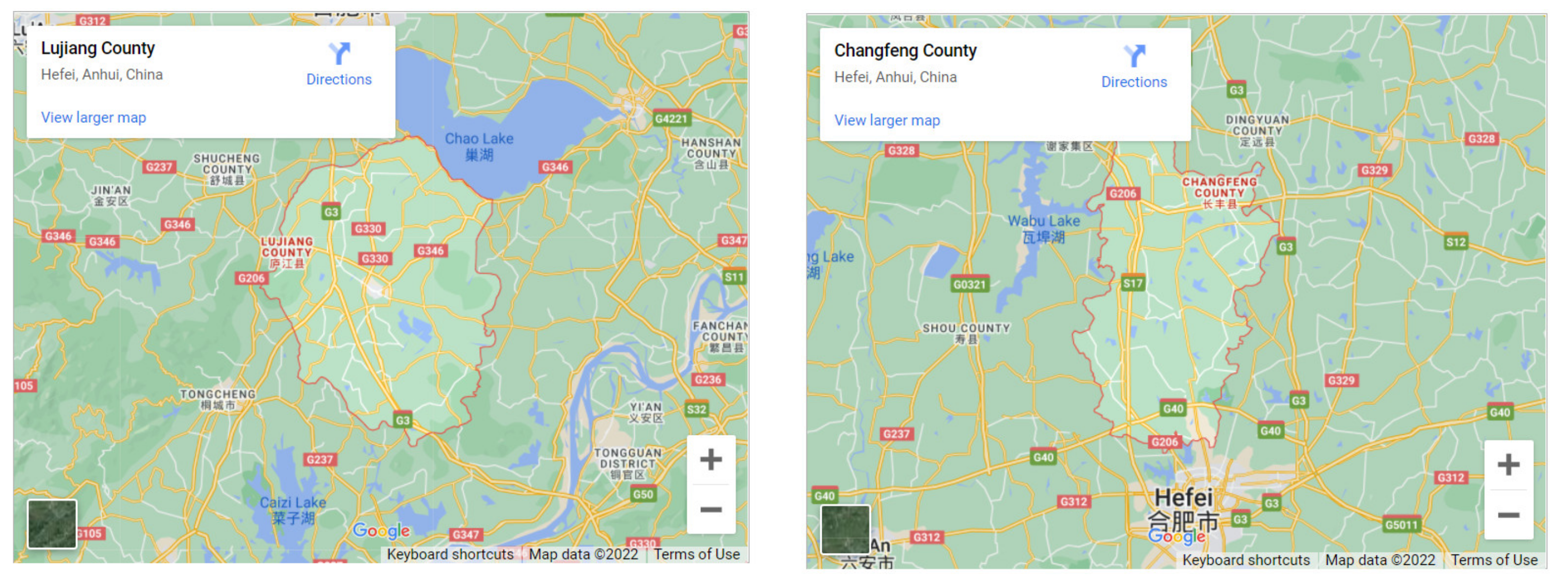
4.1. Experimental Design

In this work, the paddy fields in Changfeng County and Lujiang County of Anhui Province are selected to conduct a CCPP simulation experiment based on an improved backtracking method. Firstly, Google Maps are used to obtain the geodetic coordinates of the farmland, and the geodetic coordinates are transformed to plane coordinates according to the coordinate conversion in the same coordinate system. Then, the Canny edge detection operator was used to identify the boundaries of the farmland map. Next, the working and the obstacle areas of the farmland were processed separately to obtain a binary image of the map. The obtained binary image was mapped to the plane coordinate system using the coordinate mapping formulas. Finally, based on the processed farmland map, the traditional backtracking method, and the improved backtracking method for the CCPP were compared in the simulation experiments, and the experimental results are analyzed.

4.2. Complete Coverage Path Planning Simulation Based on Backtracking Method

Combining the actual farmland in China, the farmland in Google Maps were selected for simulation, and the CCPP of rice-transplanting IAM was realized. The farmland areas with obstacles were selected for actual measurements, and then simulation experiments were conducted. The WGS-84 geocentric geodetic coordinate system was adopted and Gaussian projection was used to transform the geodetic coordinates into a plane coordinate system [31,32].

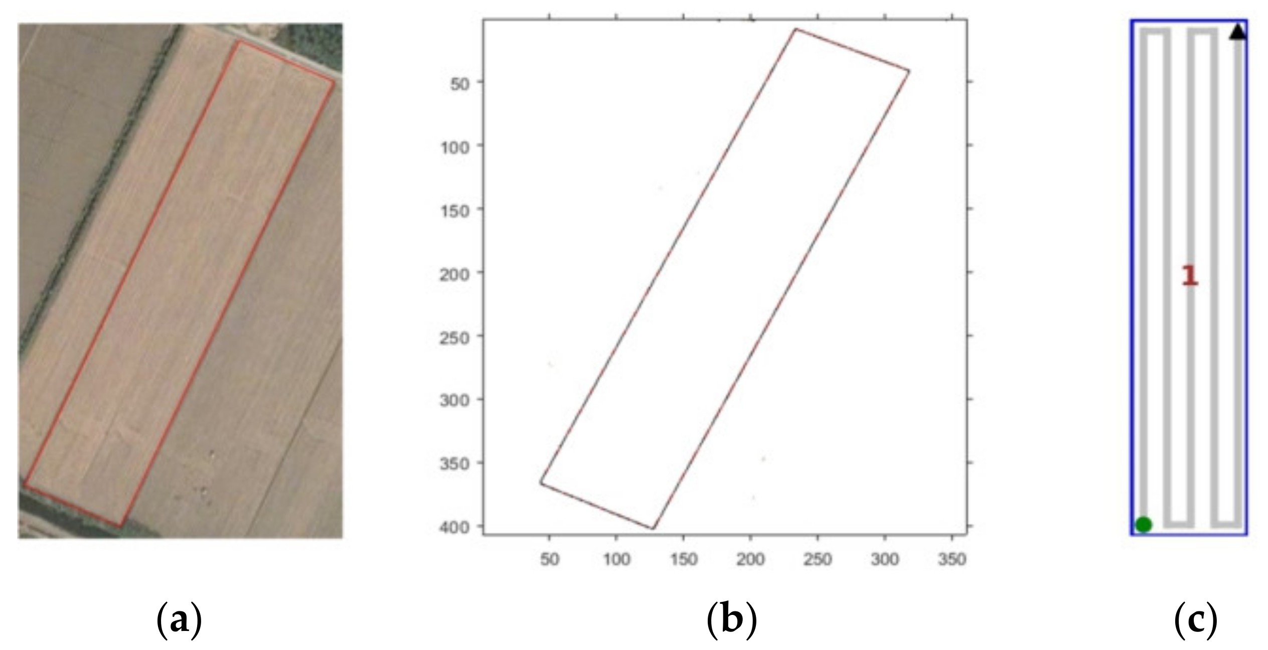
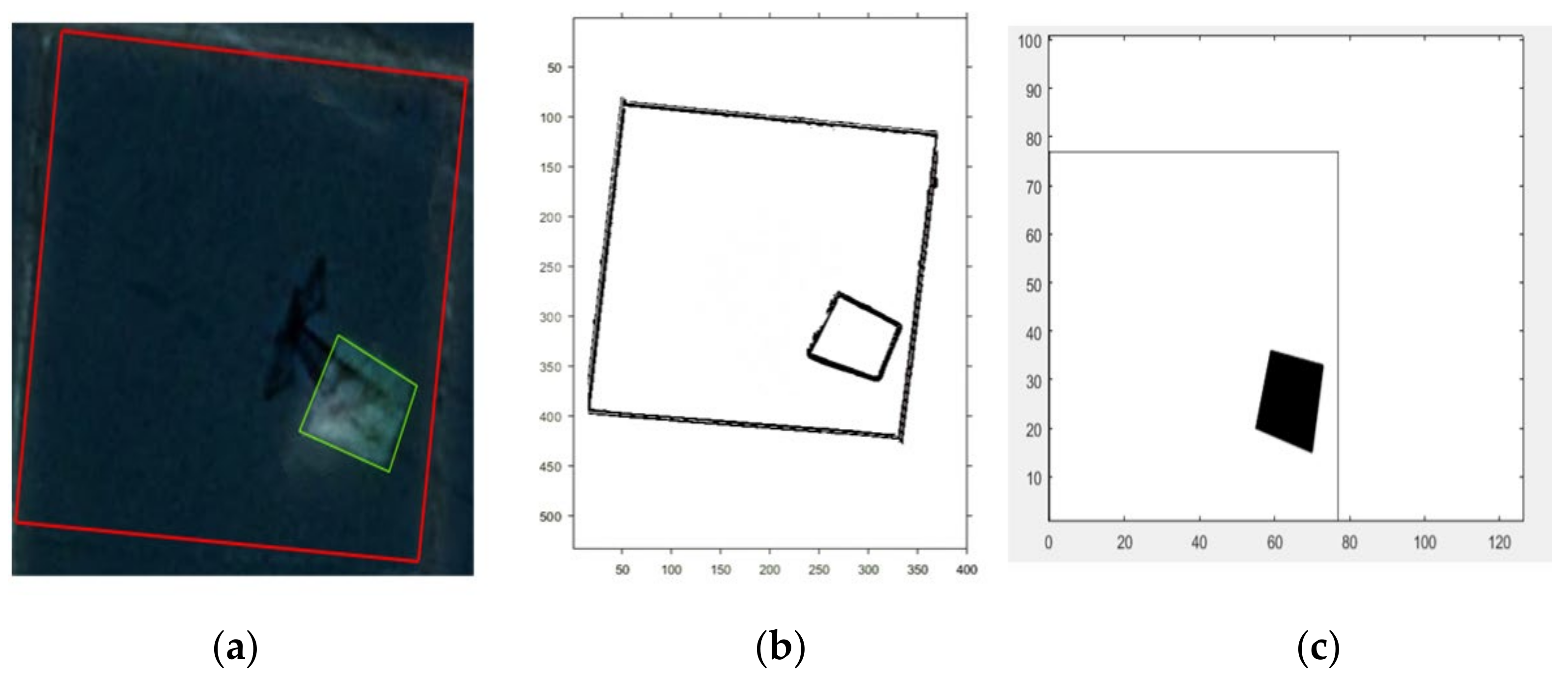
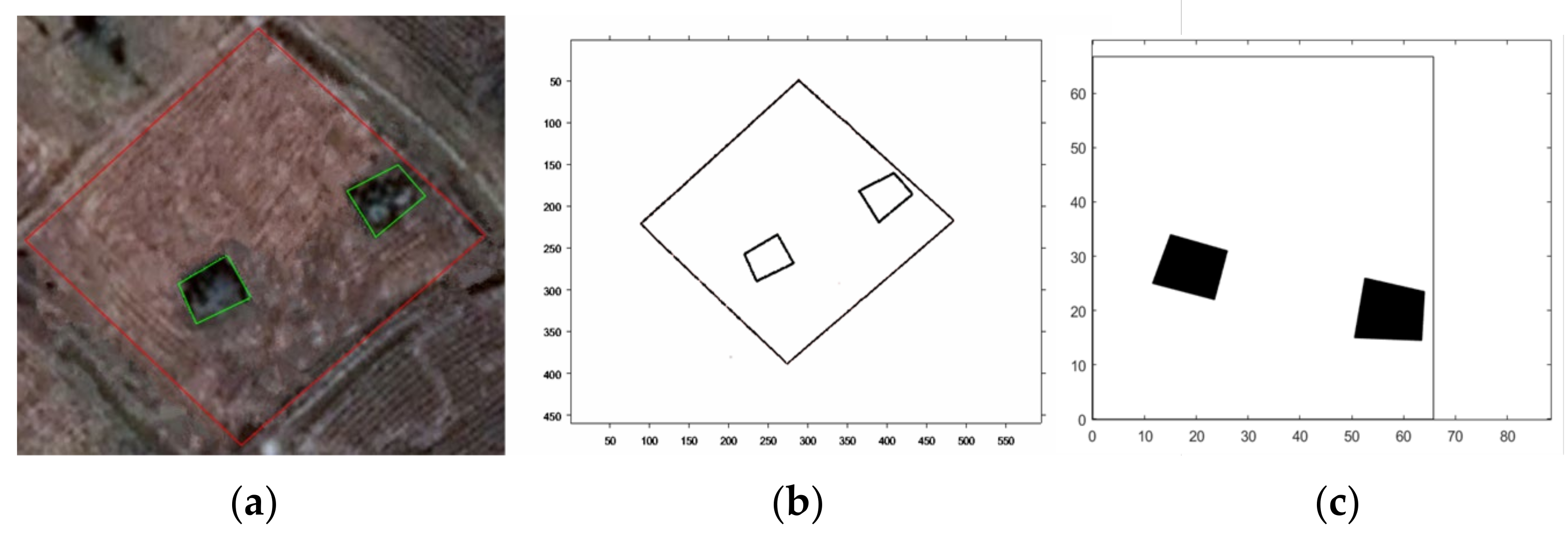
4.2.1. Coordinate System Transformation

(1) Transformation model between geodetic coordinate system and plane rectangular coordinate system.

For the transformation between the geodetic coordinate system and the plane rectangular coordinate system, the projection transformation method was adopted. the Gaussian projection was used [33,34]. The geodetic coordinates (l, B) can be transformed into plane coordinates; the formulas are as follows:

$$\left\{\begin{array}{c}x=X+\frac{N}{2}t\ast {cos}^{2}B\ast l^2+\frac{N}{24}t\left(5-t^2+9{\eta }^2+4{\eta }^4\right){cos}^{4}B\ast l^4+\frac{N}{720}t\left(61-58t^2+t^4\right){cos}^{6}B\ast l^6\\ y=N\ast cosB\ast l+\frac{N}{6}\left(1-t^2+{\eta }^2\right){cos}^{3}B\ast l^3+\frac{N}{120}\left(5-18t^2+t^4-14{\eta }^2-58{\eta }^2{t}^2\right){cos}^{5}B\ast l^5\end{array}\right.$$

(8)

$$X=c\left[{\beta }_{0}B+\left({\beta }_{2}cosB+{\beta }_4{cos}^{3}B+{\beta }_6{cos}^{5}B+{\beta }_8{cos}^{7}B\right)sinB\right]$$

(9)

$$\left\{\begin{array}{l}{\beta }_0=1-\frac{3}{4}e{{}^{\prime }}^2+\frac{45}{64}e{{}^{\prime }}^4-\frac{175}{256}e{{}^{\prime }}^6+\frac{11,025}{16,384}e{{}^{\prime }}^8\\ {\beta }_2={\beta }_0-1\\ {\beta }_4=\frac{45}{64}e{{}^{\prime }}^4-\frac{175}{256}e{{}^{\prime }}^6+\frac{11,025}{16,384}e{{}^{\prime }}^8\\ {\beta }_6=-\frac{175}{256}e{{}^{\prime }}^6+\frac{11,025}{16,384}e{{}^{\prime }}^8\\ {\beta }_8=\frac{315}{1024}e{{}^{\prime }}^8\end{array}\right.$$

(10)

In the formulas, $t=tanB, \eta =e{}^{\prime }cosB$, $l=\frac{\left(L-L_0\right){}^{″}}{\rho {}^{″}}$.

(2) Coordinate mapping formula.

The coordinates of the farmland and the obstacles in the rectangular coordinate system are expressed, respectively, as {(x_i, y_i)|i = 1, …, n}, {(x_objj, y_objj)|j = 1, …, m}. The formulas for the coordinate mapping of the farmland plane coordinates are as follows:

$$\left\{\begin{array}{ll}\left(x_i^{\prime },y_i^{\prime }\right)=\left(0,0\right)& i=1\\ \left(x_i^{\prime },y_i^{\prime }\right)=\left(x_i-x_1,y_i-y_1\right)& i\le n\\ \left(x_{objj}^{\prime },y_{objj}^{\prime }\right)=\left(x_{obj1}-x_1,y_{obj1}-y_1\right)& j\le m\end{array}\right.$$

(11)

4.2.2. Complete Coverage Path Planning in Simple Regions

Most farmland areas are simple regions. For Figure 7a, Formulas (7)–(10) are used to transform the geodetic coordinates of the farmland area into plane coordinates. The obtained coordinates are shown in

Table 1. Geodetic and plane coordinates of farmland area.

Geodetic Coordinates of Farmland Area	Plane Coordinates of Farmland Area/m
(117.482417, 31.312849) (117.483318, 31.312491) (117.481250, 31.308600) (117.480340, 31.308958)	(10,418,301.47, 3,574,527.66) (10,418,046.35, 3,574,385.17) (10,418,290.09, 3,574,639.22) (10,418,057.64, 3,574,272.57)

.

Then, the Canny edge detection operator are used to identify the boundaries of the farmland area and the obstacles from the original map information, and the binary image is obtained as shown in Figure 7b. The simulation map is established, and the result of CCPP is shown in Figure 7c.

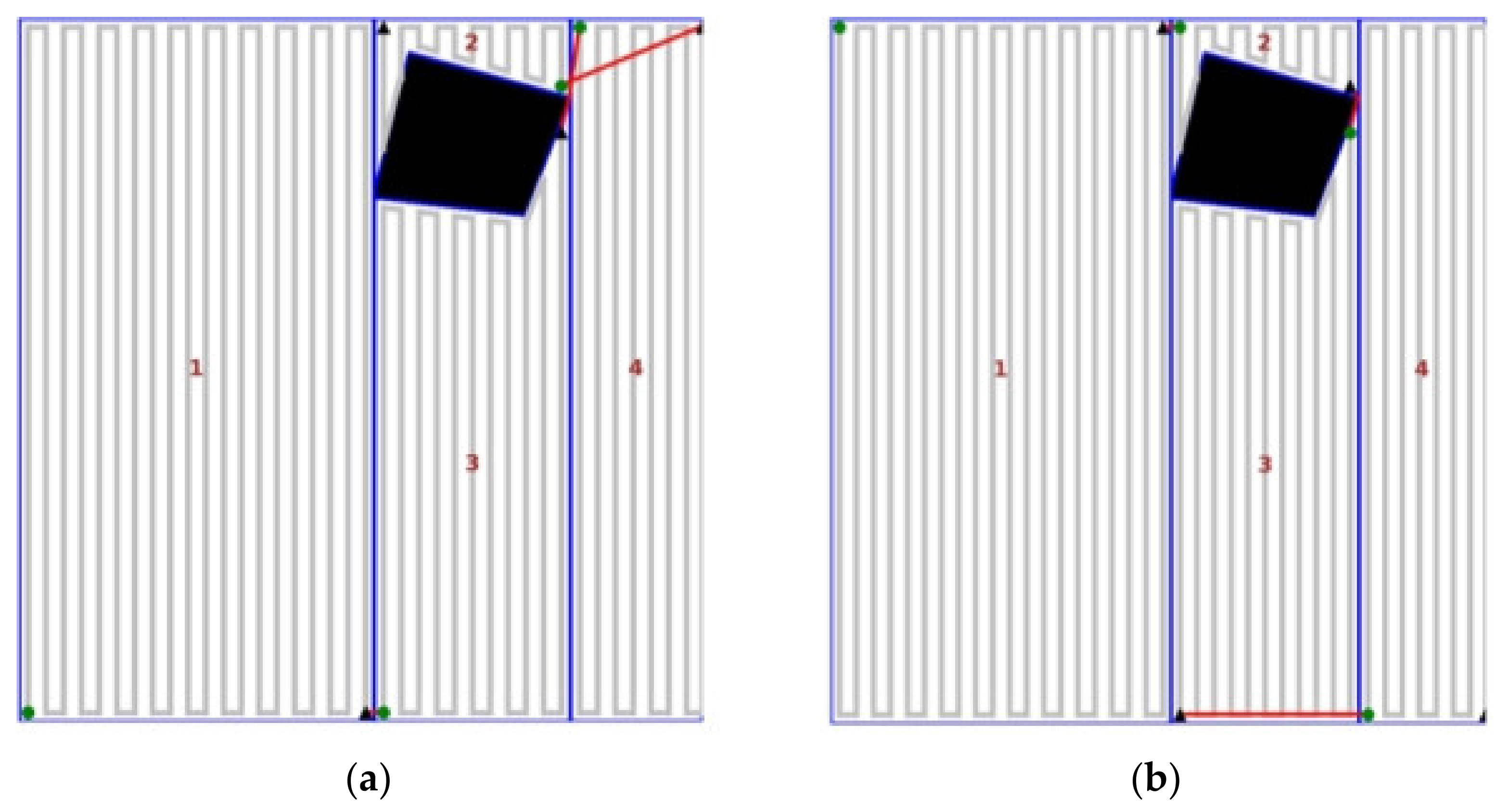
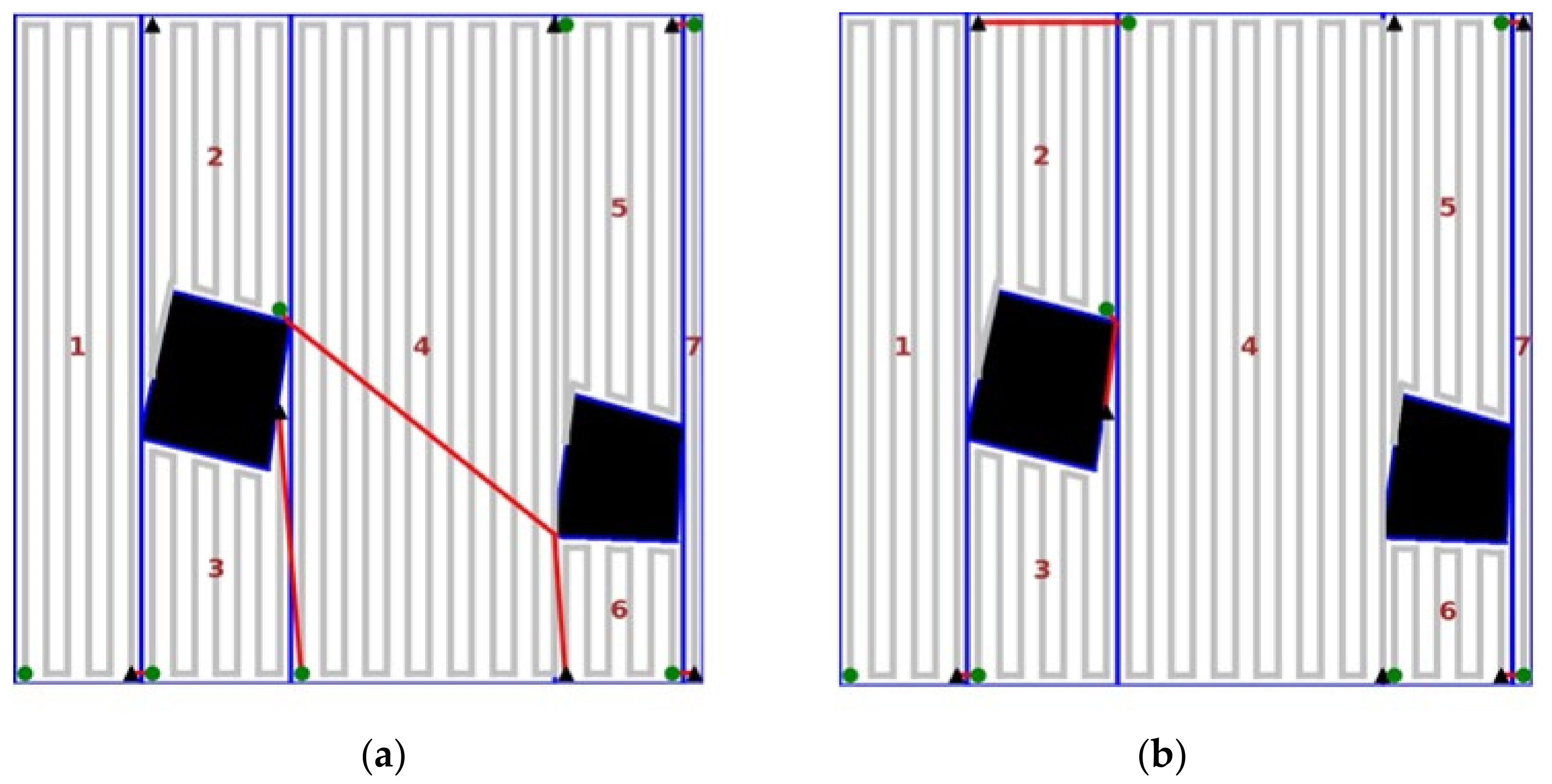
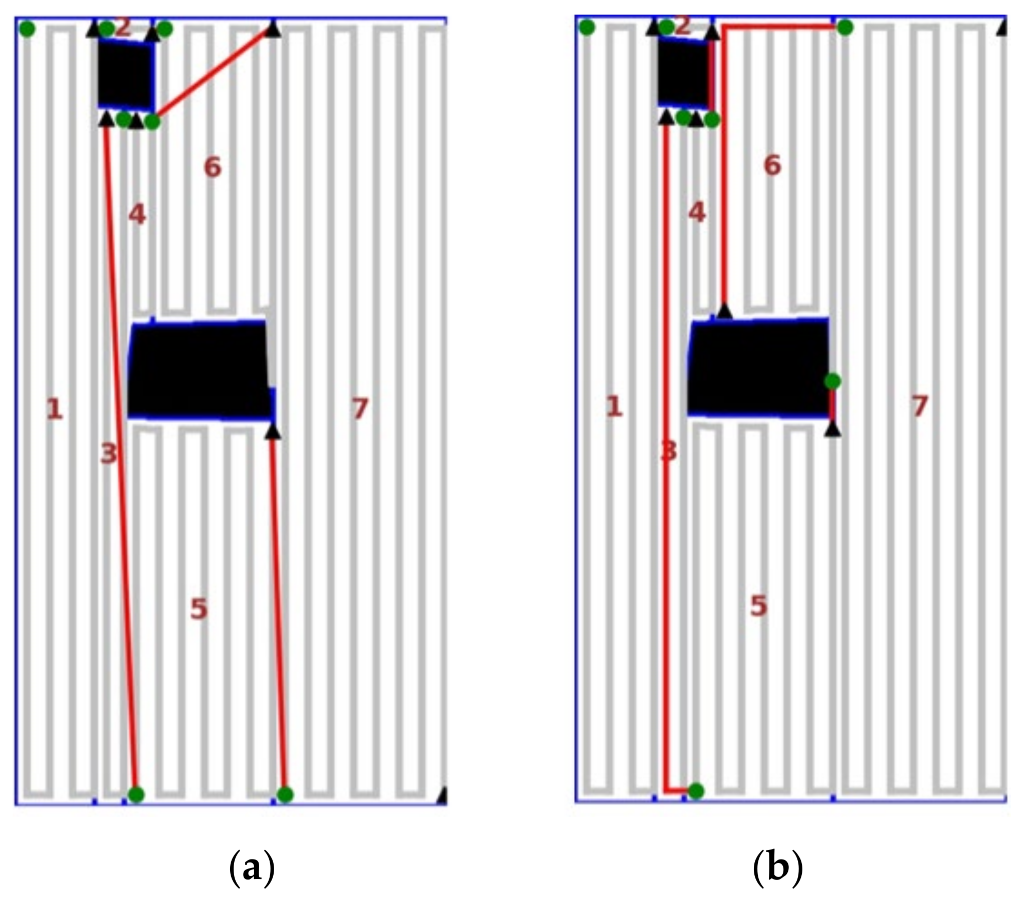
4.2.3. Complete Coverage Path Planning in Complex Regions

The paddy fields in Lujiang County and Changfeng County in Anhui Province are selected as the experimental objects from Google Maps and the situation of obstacles in the farmland area are discussed in the following categories, as shown in Figure 8.

(1) For a single obstacle in the farmland, an experimental analysis and discussion are carried out. Firstly, the Canny edge detection operator is used to recognize the farmland map. Then, one can identify the boundaries and obstacles of the farmland map and mark them as shown in Figure 9a. According to Google Maps, the geodetic coordinates of each vertex of the farmland area are shown in

Table 2. Geodetic coordinates of Figure 9a.

Geodetic Coordinates of Farmland Area	Geodetic Coordinates of Obstacle
(117.522821, 31.334724) (117.523612, 31.334646) (117.523580, 31.333977) (117.522739, 31.334032)	(117.5233953, 31.334298) (117.5235590, 31.334226) (117.5234999, 31.334107) (117.5233149, 31.334163)

. Secondly, Formulas (7)–(10) are used to transform the geodetic coordinates into plane coordinates as shown in Figure 9b, and obtain the coordinates of the farmland area and obstacles as shown in

Table 3. Plane coordinates of Figure 9a.

Plane Coordinates of Farmland Area	Plane Coordinates of Obstacle
(10,419,965.04, 3579533.91) (10,419,968.59, 3579611.79) (10,419,929.88, 3579628.13) (10,419,924.50, 3579504.08)	(10,419,946.42, 3,579,585.14) (10,419,943.95, 3,579,605.42) (10,419,936.52, 3,579,598.16) (10,419,937.86, 3,579,575.25)

. The coordinates of Table 3 are mapped as shown in

Table 4. Coordinate mapping to Figure 9b.

Farmland Mapping Coordinates	Obstacle Mapping Coordinates
(0.00, 77.04) (76.29, 77.04) (75.29, 0.00) (0.00, 0.00)	(59.01, 36.20) (73.19, 33.00) (70.10, 15.30) (55.13, 20.00)

, to obtain Figure 9c.

For the farmland map shown in Figure 9c, the CCPP algorithm proposed in this paper was compared with the original algorithm to verify its effectiveness. The experimental results are shown in Figure 10.

(2) In view of the existence of multiple obstacles, a farmland area is selected. The Canny edge detection operator is used to perform image recognition on the area of farmland and mark the boundaries and obstacles as shown in Figure 11a. According to the map, the geodetic coordinates of each vertex and obstacle of the farmland area are obtained, as shown in

Table 5. Geodetic coordinates of Figure 11a.

Geodetic Coordinates of Farmland Area Geodetic	Coordinates of Obstacle 1	Coordinates of Obstacle 2
(117.401770, 32.336933) (117.402282, 32.337332) (117.402810, 32.336922) (117.402242, 32.336562)	(117.402495, 32.337012) (117.402670, 32.337025) (117.402670, 32.337021) (117.402565, 32.336948)	(117.402117, 32.336853) (117.402224, 32.336905) (117.402278, 32.336844) (117.402147, 32.336792)

. Table 5 is used to obtain the plane coordinates according to Formulas (7)–(10), as shown in

Table 6. Plane coordinates of Figure 11a.

Plane Coordinates of Farmland Area Plane	Coordinates of Obstacle 1	Coordinates of Obstacle 2
(10,475,805.96, 3,563,281.35) (104,75,835.47, 3,563,343.54) (10,475,819.18, 3,563,409.42) (10,475,790.42, 3,563,345.22)	(10,475,820.10, 3,563,370.45) (10,475,823.17, 3,563,391.97) (10,475,822.95, 3,563,391.97) (10,475,817.40, 3,563,379.20)	(10,475,806.03, 3,563,324.24) (10,475,810.41, 3,563,337.31) (10,475,807.66, 3,563,344.09) (10,475,806.94, 3,563,328.07)

. The resulting farmland map is shown in Figure 11b. According to Formula (11), the coordinates of Table 6 are mapped to obtain

Table 7. Coordinate mapping to Figure 11b.

Farmland Mapping Coordinates Mapping	Coordinates of Obstacle 1	Coordinates of Obstacle 2
(0.00, 66.73) (65.76, 66.73) (65.76, 0.00) (0.00, 0.00)	(50.49, 15.00) (61.50, 14.50) (62.05, 23.50) (52.50, 26.10)	(11.52, 25.10) (23.50, 22.02) (26.00, 31.00) (15.00, 34.10)

, and the obtained map is shown in Figure 11c.

For the farmland map shown in Figure 11c, the CCPP algorithm proposed in this paper was compared with the original algorithm to verify its effectiveness. The experimental results are shown in Figure 12.

(3) In view of the intermediate region where there are multiple obstacles, the geodetic coordinates of the farmland area are selected and the plane coordinates are obtained according to the Formulas (7)–(10), as shown in

Table 8. Geodetic coordinates of Figure 13a.

Geodetic Coordinates of Farmland Area	Geodetic Coordinates of Obstacle 1	Geodetic Coordinates of Obstacle 2
(117.365570, 32.261266) (117.365919, 32.261402) (117.366302, 32.260874) (117.365919, 32.260717)	(117.365646, 32.261252) (117.365689, 32.261280) (117.365715, 32.261234) (117.365671, 32.261215)	(117.365795, 32.261074) (117.365920, 32.261131) (117.365959, 32.261067) (117.365836, 32.261011)

and

Table 9. Plane coordinates of Figure 13a.

Plane Coordinates of Farmland Area Plane	Coordinates of Obstacle1	Coordinates of Obstacle 2
(10,471,027.21, 3,558,980.84) (10,471,039.51, 3,559,023.52) (10,471,014.55, 3,559,071.70) (10,471,000.65, 3,559,024.87)	(10,471,027.42, 3,558,990.27) (10,471,029.57, 3,558,995.50) (10,471,027.29, 3,558,998.72) (10,471,025.63, 3,558,993.32)	(10,471,019.26, 3,559,008.90) (10,471,024.13, 3,559,024.18) (10,471,021.01, 3,559,029.10) (10,471,016.22, 3,559,014.08)

. The image identified and processed by the Canny edge detection operator is shown in Figure 13b, the coordinate mapping is shown in

Table 10. Coordinate mapping to Figure 13b.

Farmland Mapping Coordinates	Mapping Coordinates Obstacle 1	Mapping Coordinates Obstacle 2
(0.00, 69.60) (38.62, 69.60) (38.62, 0.00) (0.00, 0.00)	(7.12, 66.25) (11.80, 62.80) (11.80, 60.60) (7.12, 60.07)	(10.43, 41.70) (22.53, 42.50) (23.50, 34.52) (9.40, 33.81)

, and the map is shown in Figure 13c. The priority principle is used and the strategy of moving along the edge is adopted to achieve CCPP. Then it is compared with the traditional CCPP, as shown in Figure 14.

(4) Simulation analysis of CCPP in a complex region.

The advantages and disadvantages of the algorithm are analyzed based on the experimental simulation results through comparative analysis with the traditional backtracking method. In order to better explain the advantages of the algorithm proposed, and to make the analysis process simple and clear, three sets of farmland map models are selected with which to analyze the experimental results for the number of obstacles in the farmland. The simulation results of the two algorithms are shown in

Table 11. Experimental results.

	Backtracking Method	Search Time/s		Number of Sub-Regions Passing Through		Number of Backtracking Points		Path Length/m
Map		T	I	T	I	T	I	T	I
Group1 (Figure 10) Group2 (Figure 12) Group3 (Figure 14)		18.5 55.2 14.2	17.4 54.5 14.5	1 3 3	0 0 0	12 24 24	4 7 7	3603.60 2095.98 1506.01	3180.80 1991.98 1681.28

. In Table 11, T means traditional backtracking method and I means improved CCPP.

For the farmland map with a single obstacle (Group 1), Figure 10a shows the results of the traditional backtracking method for the simulation experiments and Figure 10b shows the results of the improved CCPP for the simulation experiments. The analysis of the simulation results of Group 1 in Table 11 shows that the traditional backtracking method will traverse a sub-region, whereas the improved CCPP does not need to traverse the sub-region. Compared with the traditional backtracking method, the number of backtracking points is significantly decreased by about 66.67%. The total path length is decreased by about 11.73%. The search time is decreased by about 5.95%. It can be seen that the improved backtracking mechanism can obtain better backtracking points by recording the uncovered sub regions in the process of regional convergence. By reducing the number of backtracking points, the length and efficiency of path planning have been improved accordingly.

For the farmland map with multiple obstacles and no intermediate region (Group 2), Figure 12a shows the results of the traditional backtracking method for the simulation experiments and Figure 12b shows the results of the improved CCPP for the simulation experiments. The analysis of the simulation results of Group 2 in Table 11 shows that the traditional backtracking method will traverse sub-regions 3 times, whereas the improved CCPP does not need to traverse the sub-region and only needs to walk along obstacles or the edge of the field. Compared with the traditional backtracking method, the number of backtracking points is significantly decreased by about 70.83%. The total path length is decreased by about 4.96%. The search time is decreased by about 1.27%. It can be seen that the behavior of crossing sub-regions is avoided. In agricultural production, such as rice transplanting, this strategy can prevent the seedlings from being damaged by agricultural machinery.

For the farmland map with multiple obstacles and at least 1 intermediate region (Group 3), Figure 14a shows the results of the traditional backtracking method for the simulation experiments and Figure 14b shows the results of the improved CCPP for the simulation experiments. The analysis of the simulation results of Group 3 in Table 11 shows that the traditional backtracking method will traverse sub-regions 3 times, whereas the improved CCPP does not need to traverse the sub-region and only needs to walk along obstacles or the edge of the field. Compared with the traditional backtracking method, the number of backtracking points is significantly decreased by about 70.83%. The total path length is increased by about 11.64% and the search time is increased by about 2.11%. It can be seen that although the number of backtracking points is significantly decreased, the search time is increased due to the avoidance of crossing the sub-region, which also leads to the longer path. But the cost is acceptable because the behavior of crossing sub-regions is avoided. Through the above comparison and analysis, the improved backtracking method that sacrificed the shorter path length to obtain the path along the boundary is chosen.

Through the comparative analysis of the experimental results, the improved CCPP algorithm has fewer backtracking points, fewer crossing sub-regions, and a lower repetition rate than the traditional backtracking method. Among these, the smaller number of backtracking points indicates that IAM has less time to select backtracking points during operation, and thus the running time is always shorter. Most importantly, the improved CCPP algorithm has fewer crossing sub-regions than the traditional backtracking method, which is more in line with the requirements of agronomy. It can be seen that the improved CCPP algorithm performs efficiently, reduces the loss by IAM in the process of agricultural cultivation activities, and adapts to complex farmland environment.

5. Conclusions

In order to solve the existing problems of CCPP algorithms for IAM, combined with the actual needs of IAM for planting seedlings, an improved CCPP algorithms based on backtracking is proposed. This method proposes ideas that improve four aspects: repeated coverage, search efficiency, path planning, and sub-regional crossing. In order to achieve an effective path with less cross sub-regions, an improved backtracking method was proposed based on the original backtracking method in the connecting process of the sub-regions combined with the needs of planting seedlings. In order to improving the efficiency of repeated coverage, the principle of priority in the intermediate region and moving along the side of farmland boundary region has been proposed. For the farmland with single obstacle, the method of moving along the boundary is proposed to reduce the repeated coverage rate in the process of traversing the next region. Regarding the intermediate region that may be generated by multiple obstacles, a strategy of priority movement in the intermediate region was proposed in order to avoid missing coverage and a second crossing of the traversed region, which will damage the seedlings that have been planted in the farmland. In terms of improving search efficiency, the backtracking points selection principle is proposed to record their own vertex of each region, which greatly reduces the calculation time of backtracking points. The experimental results show that the number of backtracking points is decreased by about 70% and the occurrence of crossing sub-regions has been significantly reduced. The improved algorithm improves the efficiency of CCPP and is more in line with the actual needs of IAM operations.

Combining the actual needs of IAM and future development trends, several suggestions are made for future CCPP research. First, when improving the CCPP algorithm of IAM, this proposed CCPP method only considers static obstacles in the farmland environment. However, there may be dynamic obstacles in reality. In the future, the operator of dynamic obstacle avoidance needs to be added to the algorithm. Secondly, when the farmland environment is unknown or partly unknown, it is necessary to integrate sensor technology to achieve “online” CCPP research. Finally, an integrated software platform should be build including environmental information processing, regional decomposition, regional connection, path planning, and experimental verification in real IAM operations should be carried out.

References

1. Liu, C.L.; Lin, H.Z.; Li, Y.M.; Gong, L.; Miao, Z.H. Analysis on Status and Development Trend of Intelligent Control Technology for Agricultural Equipment. Trans. Chin. Soc. Agric. Mach. 2020, 51, 1–18. [Google Scholar]
2. Le, A.V.; Ku, P.C.; Than, T.T.; Huu, K.N.N.; Shi, Y.; Mohan, R.E. Realization Energy Optimization of Complete Path Planning in Differential Drive Based Self-Reconfigurable Floor Cleaning Robot. Energies 2019, 12, 1136. [Google Scholar] [CrossRef] [Green Version]
3. Morimoto, E.; Hayashi, K. Design of smart agriculture Japan model. Adv. Anim. Biosci. 2017, 8, 713–717. [Google Scholar] [CrossRef]
4. Xie, B.; Wu, Z.B.; Mao, E.R. Development and prospect of key technologies on agricultural tractor. Trans. Chin. Soc. Agric. Mach. 2018, 4, 1–17. [Google Scholar]
5. Du, Y.F.; Fu, S.H.; Mao, E.R.; Zhu, Z.X.; Li, Z. Development Situation and Prospects of Intelligent Design for Agricultural Machinery. Trans. Chin. Soc. Agric. Mach. 2019, 50, 1–17. [Google Scholar]
6. Zhang, M.; Ji, Y.H.; Li, S.C.; Cao, R.Y.; Xu, H.Z.; Zhang, Z.Q. Research Progress of Agricultural Machinery Navigation Technology. Trans. Chin. Soc. Agric. Mach. 2020, 51, 1–18. [Google Scholar]
7. Dong, S.; Yuan, Z.H.; Gu, C.; Yang, F. Research on intelligent agricultural machinery control platform based on multi-discipline technology integration. Trans. Chin. Soc. Agric. Eng. 2017, 33, 1–11. [Google Scholar]
8. Xu, B.; Xu, M.; Chen, L.P.; Tan, Y. Review on Coverage Path Planning Algorithm for Intelligent Machinery. Comput. Meas. Control 2016, 24, 1–5. [Google Scholar]
9. Ma, Y.F.; Sun, H.; Ye, P.; Li, C. Mobile robot multi-resolution full coverage path planning algorithm. In Proceedings of the 2018 5th International Conference on Systems and Informatics (ICSAI), Nanjing, China, 10–12 November 2018; pp. 120–125. [Google Scholar]
10. Peng, Y.; Bao, L.Z.; Qu, D.; Xie, Y.M. Global Path Planning Algorithm of Multi-Bug. Trans. Chin. Soc. Agric. Mach. 2020, 51, 375–384. [Google Scholar]
11. Oksanen, T.; Visala, A. Coverage path planning algorithms for agricultural field machines. J. Field Robot. 2009, 26, 651–668. [Google Scholar] [CrossRef]
12. Deng, Y.; Yang, G.W.; Cui, X.M.; Wu, S.L. Application of Improved Back Propagation Neural Network in Mowing Robot’s Path Planning. Appl. Mech. Mater. 2014, 602, 916–919. [Google Scholar] [CrossRef]
13. Khan, A.; Noreen, I.; Ryu, H.; Doh, N.L.; Habib, Z. Online complete coverage path planning using two-way proximity search. Intell. Serv. Robot. 2017, 10, 229–240. [Google Scholar] [CrossRef]
14. Hong, L.; Jiayao, M.; Weibo, H. Sensor-based complete coverage path planning in dynamic environment for cleaning robot. CAAI Trans. Intell. Technol. 2018, 3, 65–72. [Google Scholar]
15. Xu, B. Research on Route Planning for Plant Protection Unmanned Aerial Vehicles. Ph.D. Thesis, China Agricultural University, Beijing, China, 31 May 2017. [Google Scholar]
16. Wang, J.; Chen, J.; Cheng, S.; Cheng, S.; Xie, Y. Double Heuristic Optimization Based on Hierarchical Partitioning for Coverage Path Planning of Robot Mowers. In Proceedings of the International Conference on Computational Intelligence and Security, Wuxi, China, 16–19 December 2016; pp. 186–189. [Google Scholar]
17. Nakamura, K.; Nakazawa, H.; Ogawa, J.; Naruse, K. Robot sweep path planning with weak field constrains under large motion disturbance. Artif. Life Robot. 2018, 23, 532–539. [Google Scholar] [CrossRef]
18. Cao, X.; Yu, A. Complete-coverage path planning algorithm of mobile robot based on belief function. CAAI Trans. Intell. Syst. 2018, 13, 304–321. [Google Scholar]
19. Jian, Y.; Gao, B.; Zhang, Y. Study on a complete coverage path planning method for indoor cleaning robots. Transducer Microsyst. Technol. 2018, 37, 32–34. [Google Scholar]
20. Liu, C.Q.; Zhao, X.Y.; Du, Y.F.; Cao, C.; Zhu, Z.X.; Mao, E.R. Research on static path planning method of small obstacles for automatic navigation of agricultural machinery. IFAC Pap. 2018, 51, 673–677. [Google Scholar] [CrossRef]
21. Li, K.; Chen, Y.F.; Jin, Z.Y.; Liu, T.; Wang, Z.T.; Zhang, J.Z. A complete coverage path planning algorithm based on backtracking method. Comput. Eng. Sci. 2019, 41, 1227–1235. [Google Scholar]
22. Chen, C.Y.; Xiong, H.G.; Tao, Y.; Zou, Y.; Fan, R.; Jiang, S. Coverage path planning method for service robot based on efficient template algorithm and dynamic window approach. Chin. High Technol. Lett. 2020, 30, 945–958. [Google Scholar]
23. Wang, Y. Complete Coverage Path Planning of Mobile Robot for Abandoned Mine Land. Master’s Thesis, China University of Mining and Technology, Beijing, China, 2020. [Google Scholar]
24. Zhou, L.N.; Wang, Y.; Zhang, X.; Yang, C.Y. Complete coverage path planning of mobile robot on abandoned mine land. Chin. J. Eng. 2020, 42, 1200–1228. [Google Scholar]
25. Xu, K.B.; Lu, H.Y.; Huang, Y.H.; Shi, J. Robot Path Planning Based on Double-Layer Ant Colony Optimization Algorithm and Dynamic Environment. Acta Electron. Sin. 2019, 47, 2166–2176. [Google Scholar]
26. Song, X.R.; Ren, Y.Y.; Gao, S.; Chen, C.B. Survey on Technology of Mobile Robot Path Planning. Comput. Meas. Control 2019, 27, 1–5. [Google Scholar]
27. Jeong, S.; Simeone, O.; Kang, J. Mobile Edge Computing via a UAV-Mounted Cloudlet: Optimization of Bit Allocation and Path Planning. IEEE Trans. Veh. Technol. 2017, 67, 2049–2063. [Google Scholar] [CrossRef] [Green Version]
28. Samaniego, F.; Sanchis, J.; García, N.S.; Simarro, R. Recursive Rewarding Modified Adaptive Cell Decomposition (RR-MACD): A Dynamic Path Planning Algorithm for UAVs. Electronics 2019, 8, 306. [Google Scholar] [CrossRef] [Green Version]
29. Batsai khan, D.; Janchiv, A.; Lee, S.G. Sensor-Based Incremental Boustrophedon Decomposition for Coverage Path Planning of a Mobile Robot. Intell. Syst. Comput. 2013, 12, 621–628. [Google Scholar]
30. Blumenthal, A.; Latushkin, Y. The Selgrade Decomposition for Linear Semiflows on Banach Spaces. J. Dyn. Differ. Equ. 2019, 31, 1427–1456. [Google Scholar] [CrossRef] [Green Version]
31. Zhang, H.T.; Ji, M. Research on Coordinate Transformation from Local Plane Coordinate System to CGCS2000 Based on Plane Four Parameter Model. Bull. Surv. Mapp. 2018, 0, 74–77. [Google Scholar]
32. Peng, X.Q.; Gao, J.X.; Wang, J. Research of the Coordinate Conversion between WGS84 and CGCS2000. J. Geod. Geodyn. 2015, 35, 219–221. [Google Scholar]
33. Gong, X.C.; Zhiping, L.; Wang, Y.P.; Hao, L.; Wang, N. Comparison of Calculation Methods of Several Coordinate Transformation. J. Geod. Geodyn. 2015, 35, 697–701. [Google Scholar]
34. Deng, Y.H. 2D Coordinate Transformations with Improved Total Least Square Method. J. Geod. Geodyn. 2016, 36, 162–166. [Google Scholar]
Figure 1. (a) Environment map; (b) connected graph of generated from (a); (c) CCPP based on backtracking method.
Information 13 00313 g001aInformation 13 00313 g001b
Figure 2. (a) Environment map; (b) Morse decomposition.
Information 13 00313 g002
Figure 3. Round-trip traversal path planning.
Information 13 00313 g003
Figure 4. Adjacent region. (a) Right adjacent region. (b) Left adjacent region.
Information 13 00313 g004
Figure 5. (a) Moving along the inner boundary; (b) moving along the outer boundary.
Information 13 00313 g005
Figure 6. Flow chart of CCPP based on backtracking method.
Information 13 00313 g006
Figure 7. (a) The farmland map; (b) The map after binarization; (c) CCPP for simple regions.
Information 13 00313 g007
Figure 8. The location of Lujiang County and Changfeng County on the map.
Information 13 00313 g008
Figure 9. (a) Farmland map. (b) map after binarization. (c) coordinate mapping to (b). The red square is the boundary of the farmland area, and the green square is the boundary of the obstacle.
Information 13 00313 g009
Figure 10. (a) Traditional CCPP; (b) improved CCPP. In the figure, the green dots represent the starting point of each sub-region and the black triangle represents the finishing point of each region. The red lines are the route connecting sub-regions.
Information 13 00313 g010
Figure 11. (a) Farmland map with obstacles; (b) map after binarization; (c) coordinate mapping to (b).
Information 13 00313 g011
Figure 12. (a) Traditional CCPP; (b) improved CCPP. In the figure, the green dots represent the starting point of each sub-region and the black triangle represents the finishing point of each region. The red lines are the route connecting sub-regions.
Information 13 00313 g012
Figure 13. (a) Farmland map with obstacles; (b) map after binarization; (c) coordinate mapping to (b).
Information 13 00313 g013
Figure 14. (a) Traditional CCPP; (b) improved CCPP. In the figure, the green dots represent the starting point of each sub-region and the black triangle represents the finishing point of each region. The red lines are the route connecting sub-regions.
Information 13 00313 g014