Article

Travel-Time Estimation by Cubic Hermite Curve

by
Owen Tamin
1,2,
Badrul Ikram
1,
Ahmad Lutfi Amri Ramli
1,
Ervin Gubin Moung
2,* and
Christie Chin Pei Yee
2
1
School of Mathematical Sciences, Universiti Sains Malaysia, Gelugor, Penang 11800, Malaysia
2
Faculty of Computing and Informatics, Universiti Malaysia Sabah, Kota Kinabalu, Sabah 88400, Malaysia
*
Author to whom correspondence should be addressed.
Information 2022, 13(7), 307; https://doi.org/10.3390/info13070307
Submission received: 25 May 2022 / Revised: 10 June 2022 / Accepted: 17 June 2022 / Published: 23 June 2022
(This article belongs to the Special Issue Soft Computing in Intelligent Transportation System)

Abstract

:
Travel time is a measure of time taken to travel from one place to another. Global Positioning System (GPS) navigation applications such as Waze and Google Maps are easily accessible presently and allow users to plan a route based on travel time from one place to another. However, these applications can only estimate general travel time based on a vehicle’s total distance and average safe speed without considering route curvature. A parametric cubic curve has shown a potential result in travel-time estimation through geometric properties. In this paper, travel time has been estimated using the curvature value obtained from the Hermite Interpolation curve fitted to each section of the selected road. Design speed is determined from the curvature value, and thus an algorithm for travel-time estimation incorporating initial driving information is developed. The proposed method’s accuracy was compared to the existing method’s accuracy using a real-life driving test. This comparison demonstrated that the proposed method estimates travel time more accurately than Google Maps and Waze. Future study can further improve the estimation by embedding traffic data into the algorithm.

1. Introduction

The emergence of the Global Positioning System (GPS) navigation system with cutting-edge map technology has throughout the last decade significantly impacted how road users travel. For years, road drivers have leveraged GPS applications such as Google Maps and Waze to reduce their travel time by obtaining the best route suggestion with an estimated travel time [1]. Travel time is generally a measure of time taken to travel from one place to another. The GPS applications calculate estimated travel time based on the distance between two points and the average speed limit, as well as current traffic conditions [2]. They also collect traffic data on the speed limits of major highways, freeways, and streets. Although GPS applications rely heavily on traffic data, the accuracy of the estimated travel time may be affected in locations where traffic data are limited, such as in rural areas. Prior studies have shown that the estimation of travel time in rural areas can be calculated by implementing Markov Chains, which rely on traffic flow data from microwave detectors as one of their primary sources [3]. The modified Bayesian data fusion model collects data from loop detector data, GPS data, historical data, and ground truth data [4].
Current approaches for calculating travel time based on GPS data have their own limitations. For instance, they are less effective in handling difficulties linked to GPS and spatial road network data uncertainties, such as time window length, vehicle penetration rate, sampling frequency, and vehicle coverage on the network. Furthermore, they are more likely to rely on higher-frequency data sources from specialist data providers, which can be costly and not always available [5]. GPS applications do not consider driving speed and the curvature of the road in predicting the estimated travel time. Heavily relying on GPS alone will result in inconsistent travel-time estimation on different routes. Especially in locations where GPS data or historical travel data cannot be relied on, the road properties can give a valuable indicator of how fast a car travels on a particular road. Therefore, driving speed and road curvature can be introduced as part of the solution in overcoming the limitations faced by other existing methods in relying upon traffic data for travel-time estimation [6]. This proposed method is cheaper, more accessible and more accurate in estimating travel time.
In this paper, one type of cubic curve, the Hermite interpolation curve, is used to ensure connection and tangent continuity between segments, which is essential in visualization. Cubic curves are commonly used in graphics due to their ability to allow some flexibility in the curve design characterized by their control polygons, and compromise between flexibility and speed of computation [6]. Approximating travel time taken by an individual based on road curvature and the average speed is the aim of this study. The proposed method has the advantage of overcoming the limitation of traffic data where it is not available in certain areas, mainly rural. The proposed method can still work well in both urban and rural areas due to the reliance on calculation. Therefore, geometric properties give a better and more precise estimation of travel time than traffic data implemented in the existing system.
In summary, the significance of this study are as follows:
  • The proposed method can provide a better estimation for road users in planning their journey from the starting point to the final destination with an accurate estimated time of arrival.
  • The proposed algorithm uses geometric properties of the road, which is the curvature value instead of traffic data. This value will estimate the maximum driving speed for a particular section of the road to be embedded in the travel-time estimation based on the initial driving information.
The significance of the study described above is listed in the first section of this paper. The literature review for this study is discussed in Section 2, and the research methodology is outlined in Section 3. The results are then reviewed in Section 4. The conclusion and prospective future works are presented in Section 5 and Section 6, respectively.

2. Literature Review

Car drivers are risk-averse when choosing a route recommended by a system with a shorter average travel time than the same route’s usual travel time. On the other hand, they tend to be risk-seeking when choosing a recommended route with a longer average travel time than the expected average travel time of the same route. This trend is repeated in driving simulation research where the reference route has a broad scope of travel time while the reference range is narrower than the range of accessible paths [7].
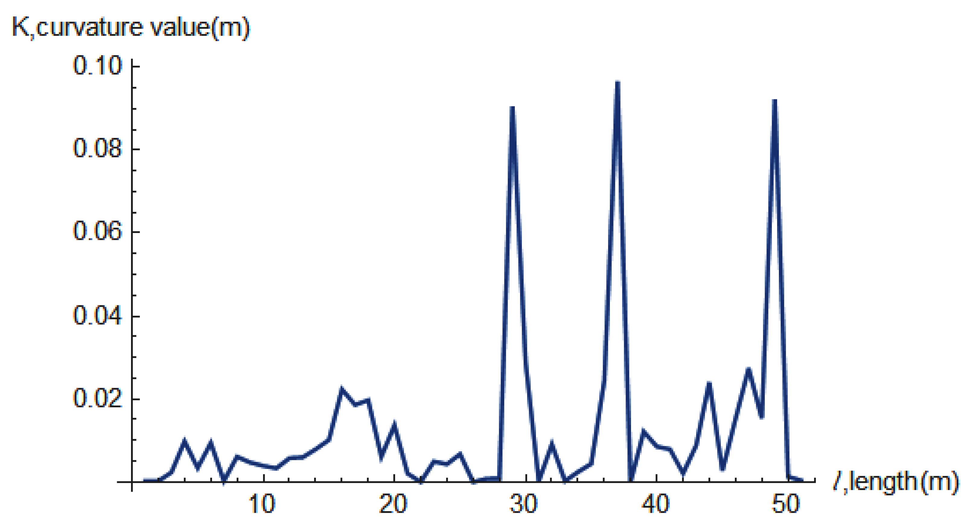
The curvature profile is the variability of the curve as a specific point that moves along the curve. The greater the curvature, the smaller the radius [8]. Naturally, curvature is a quantity that is inversely proportional to the radius of the circle. The fairness of a curve, which is related to the concept of curvature profile, can be seen by plotting the curvature versus the arc length for a given curve [8]. Thus, the curvature curve for the fair curves can be defined. This indicates that a curve is fair if its curvature plot consists of relatively few monotone pieces.
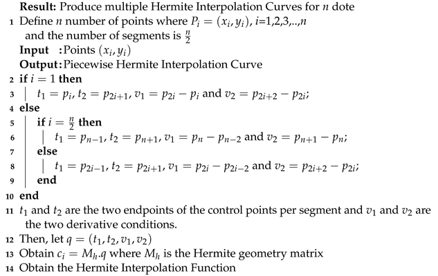
A parametric curve, such as a Hermite curve or a Bézier curve, employs a simple formula in which the curve is defined in terms of control polygons (a set of control vertices connected to form sequences or patterns). Although the curve resembles all control polygon patterns, it always interpolates the initial and final vertices [9]. The number of control polygons is equal to the number of edges in the polynomial curve.
This description states that global control is within the formulation, which means the movement of a control vertex influences the entire curve’s shape pattern. This description indicates that global control is within the formulation. As a result, the movement of a control vertex affects the overall shape pattern of the curve. Furthermore, because it is a polynomial, the curve is infinitely different.
A continuous vector function exists in a closed curve C in Euclidean n-space H n . The continuous vector function of period l, which is not constant in any t-interval, is denoted as r t = r 1 t , , r n t . It is much more convenient to assume any polygon as a closed curve and ignore the differences in parameterizations. Suppose that r t is a continuous vector function. A closed curve r t can be simplified further to r t 1 = r t 2 if t 1 t 2 l produces an integer. A closed polygon P with vertices a 1 , , a m is said to be inscribed in a closed curve r t if there is a set of parameter values t i such that t i < t i + 1 , t i + m = t i + 1 , and a i = r ( t i ) for all integral values of i. If P is a polygon with at least two coincident vertices, it can be represented as the limit of a sequence of polygons with distinct vertices. As a result, all that is left is to prove the lemma for P with all vertices distinct [10].
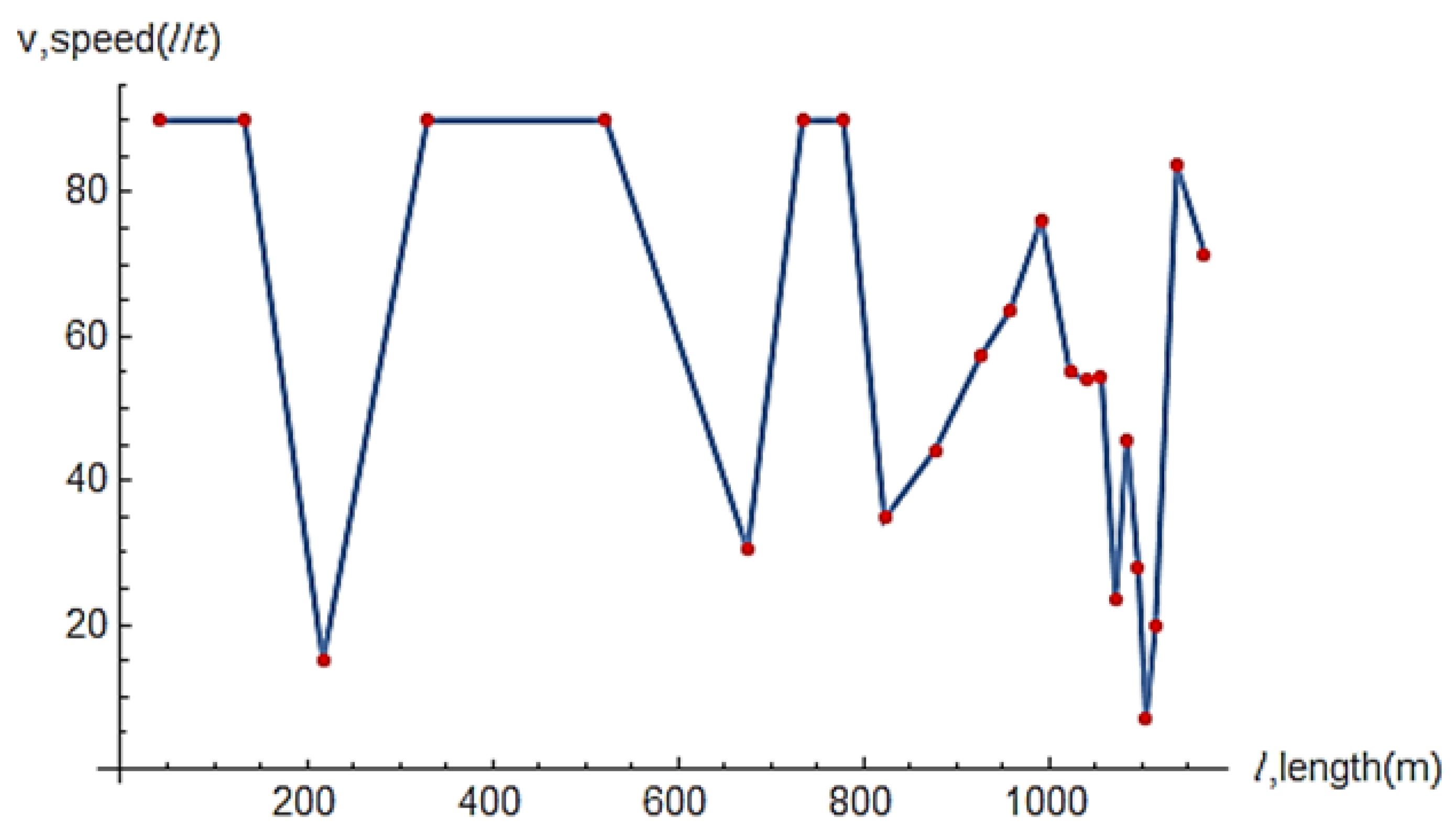
Design speed is defined as the maximum safe speed that is sustainable under ideal road conditions. This results in highway design characteristics taking precedence over a particular section of the highway. The value of design speed is ideal based on topography, neighboring land use, and highway functional classification [11]. Thus, to achieve a safe maximum speed, the design speed should take into account vehicle safety and comfortability. According to the 1936 Barnett concept of design velocity, when the urban area is cleared, the driving community of vehicle operations will tend to be faster due to the high reasonable uniform velocity. The situation will contribute to the growing crash rate when the drivers drive along the horizontal curves of the road. The main concern at the time was that the curves were designed for non-motorized or slow-moving motorized vehicles, but car manufacturers have since been able to develop automobiles capable of reaching higher speeds [12].
According to Leisch and Leisch [13], design speed is a representative operating potential velocity defined by the design and correspondence of a highway’s geometric characteristics. It indicates a nearly constant near-maximum speed that a driver on the road can comfortably maintain in good weather and with little traffic. Furthermore, it also functions as an indicator for the highway’s physical condition [13]. The design speed principle, as currently applied, does not prevent inconsistencies in highway alignment. The fundamental problem, especially in the range of design speeds below 90 km/h (55 mph), is the driver’s propensity to accelerate and decelerate continuously. The speed-profile technique can be used to resolve the speed disparity between cars and trucks, helping to meet the standards of drivers and comply with their inherent characteristics to achieve operational consistency and enhance driving comfort and safety.
Roads are constructed based on a suitable and safe design speed, which is the same for every given path in the roadway. The vehicle’s mass is assumed to be constant in the given situation, and the vehicle must be able to travel safely and comfortably at the given path of the road regardless of the bend [14]. The process of road velocity design reflects the correlation between curvature and velocity, in which the basic principle of horizontal curve design is derived from kinematic equation applications. In the 1930s, the United States designed the roadway’s vertical and horizontal alignments with design speed as the main consideration. By taking design speed into consideration, the design criteria for a new roadway were proposed to ensure the development of an appropriate horizontal curve radii, superelevation rates, and vertical curve elements.
The design criteria were suggested to develop appropriate horizontal curve radii, superelevation rates, and vertical curve elements for new roadways [11]. Simultaneously, the use of statistical analysis of the independent vehicle speeds on the freeway was introduced. There are areas in which the stated velocity limit centered on the 85th percentile speed above the roadway’s recommended design speed due to variations in design and activity requirements.
It is possible to predict general travel time for routes using traditional navigation systems. For instance, regardless of the route’s metric system, a travel time can be calculated by dividing the path’s distance by the speed limit. However, such calculations may contain errors due to road conditions, traffic congestion, driving habits, the accuracy of the navigation system, and other variables that navigation systems do not account for [15]. The real-time measurement for travel time of a single route consists of a set of multiple road sections. The development of the sections is essential for the needs of traffic control, searching for driving directions, ride-sharing, and taxi dispatch [16]. The use of loop sensors as a new technique would tell individuals the travel speed of a particular path section instead of the travel time of a full journey.
Furthermore, the use of Vehicular Ad-hoc Network (VANET) technology, optimal sensor location model, Cellular Floating Vehicle Data (CFVD), Travel-Time Variability (TTV) and Urgent-Gentle Class (UGC) traffic flow model will enable effective and efficient transportation in the city [17,18,19,20,21]. The UGC traffic flow model estimates travel time through a ring road with viscoelastic and ramp effects. This method applies mathematical modeling in travel-time estimation without traffic data. Results show that average travel time increases when the initial ring-road density increase.
Several traveler information systems have recently been developed to provide travelers with real-time traffic information. In a typical travel information system, a road map is divided into route segments. The time required for a vehicle to travel along a particular route segment is predicted using historical and real-time sensor data. On the road, travel-time predictions are based on the relationship between the distance between two points and the time required to complete the journey [22].
Over the last decade, there has been a motivation for the development and deployment of Intelligent Transportation Systems (ITS) in travel-time estimation due to the numerous advantages that these systems can primarily provide, using Bluetooth. These systems are designed to provide users with information regarding pre-trip or en route travel to help them choose the most efficient mode of transport and to ensure an optimal control strategy. Currently, most of the states in the United States provide travelers with information on current road conditions, such as speeds, travel time, incidents, and lane closures. Drivers can then be informed of their travel time via dynamic message signs, the Internet, and cell phones [23]. By analyzing information from a large sample of vehicle trips within a city, it is possible to remodel the city’s traffic pattern [24].
There may be a few factors affecting travel-time estimation based on the route traveled between two points in the network. The consistency of the range of average travel time value along the pathway is one of the factors. A study was conducted in which the movement and position of the probe vehicles within a specified interval on the road were used as the primary observation for the purpose of predicting travel time. The sampling rate is assumed to be lower due to the scale required for measuring travel time, which is shorter than the distances between consecutive records. Instantaneous speed data would not be accessible because of the communication bandwidth limitations. Within these communication bandwidth constraints, the only data available is the distance traveled and the estimated travel time [25]. Disregarding the influence of the initial travel time will undoubtedly influence the identification of the shortest route and traffic data [26].

3. Materials and Methods

The algorithm that was used to compute the Hermite interpolation function will be adapted to construct the Hermite interpolation curve using coordinates of two given routes. Furthermore, the algorithm for estimating travel time based on initial driving data will also be adapted to provide a theoretical concept for calculating curvature, design speed, and travel time estimation. Additionally, this section discusses the five stages involved in estimating travel time, as well as the overall flowchart.

3.1. Research Methodology

This section proposes a suitable algorithm for estimating travel time. An algorithm for computing the Hermite interpolation function was presented. This is followed by another algorithm that specifically estimates travel time based on initial driving information and individual driving speed profiles.

3.2. Overall Flowchart

Figure 1 shows the overall flowchart of the proposed method. The overall flowchart consists of five phases; (i) Phase A involves obtaining the route’s coordinates, (ii) Phase B details the process of calculating the curvature values and curvature radius, (iii) Phase C details the process for calculating the arc lengths of the routes, (iv) Phase D describes the process of calculating the design speed that is capped by the average speed, and finally (v) Phase E describes the process of estimating travel time. Each phase will be explained in detail using theory and a flowchart, which will be included in the following section.

3.3. Algorithm in Computing Hermite Interpolation Function

The procedure for estimating travel time is shown in Algorithm 1.
Algorithm 1: Hermite Interpolation Curve
Information 13 00307 i001

3.4. Description of Methodology

3.4.1. Phase A: Obtaining the Coordinates of the Routes’ Starting and Ending Points

Figure 2 describes the process involved in Phase A. There are several methods for obtaining the route’s coordinates. One method is to manually select the points. In this case, the points are selected by obtaining the coordinates from the image in Mathematica, where scaling is required. The coordinates obtained in units based on the map scale will then be converted to meters.
Another way to obtain coordinates is using Garmin BaseCamp as shown in Figure 3. Garmin Basecamp is a map-viewing or GIS software package primarily used with Garmin GPS navigation devices. Garmin BaseCamp is used because it can detect a significant number of point locations along the selected routes, yielding positive results in the estimation of travel time. Garmin BaseCamp records all coordinate points within a 15 to 25 m interval along the route in longitude and latitude formats.
Once the coordinates are obtained, the coordinates need to be converted into x i , y i forms. Due to the fact that the coordinates obtained from Garmin BaseCamp are in longitude and latitude formats, they must first be converted to decimal degrees before being converted to meters. The coordinates can be converted to decimal degrees by using Mathematica’s built-in function FromDMS. The formula of finding the decimal degrees, DD is given by Equation (1)
D D = d e g r e e s + ( m i n u t e s 60 ) + ( s e c o n d s 3600 )
In other words, 1 decimal degrees is equal to 1 in longitude and latitude forms. For the decimal degrees to be converted to meters, we need to use the conversion factor of 10 , 000 km per 90 degrees due to the differences of 42 km between the earth’s circumference around the equator and that around the poles. In other words, 1 m is approximately 111 , 111 decimal degrees. Thus, the coordinate points will be in x i , y i forms in meters metrics units.

3.4.2. Phase B: Calculating the Curvature Values and Radius of Curvature of the Routes

Figure 4 describes the process involved in Phase B. The curvature of the curve can then be derived by fitting the curves to the data. For every three consecutive control points of the curve, the curvature value denoted as K can be approximated for the second data points. The parameter, u, is set to be 0.5 . This variable represents the distance traveled by the curve from its starting point as a function for parametric curves with x and y coordinates. The reason for setting u to 0.5 is to minimize the error associated with estimating the curvature value of the routes, as the curve may or may not pass through the second point.
The curvature formula can be used to approximate the curvature for the second point of each curve, where the curvature at any point M t = x , y is given by Equations (2) and (3)
K = x y y x x 2 + y 2 3 2
in which the curve is defined in parametric form by the equations
x = f ( t ) , y = g ( t )
The radius of curvature, R, is the radius of an osculating circle that touches one or more curves that has the same tangent and curvature at a given point that can be determined as in Equation (4)
R = 1 K
which also known as the inverse of the curvature K of the curve at point M t = x , y . In other words, R is the inverse of K or K 1 .

3.4.3. Phase C: Calculating the Arc Length of the Routes

Figure 5 describes the process involved in Phase C. Arc length is the distance between two points along a section of a curve. The arc length value between each curve determines the distance along the curved line that forms the arc. The arc length value can be obtained using the arc length with parametric equations given by Equations (5) and (6)
L = α β d x d t 2 + d y d t 2 d t
for the domain of
α t β

3.4.4. Phase D: Calculating a Design Speed That Is Capped by the Average Speed

Figure 6 describes the process involved in Phase D. The minimum radius refers to the curvature value that cannot be exceeded at a given design speed. It depends on the maximum rate of superelevation and the maximum allowable side-friction factor. The minimum safe radius can be determined using the standard curve equation denoted by Equation (7)
R m i n = V 2 127 ( e + f )
where
Rmin = minimum radius of circular curve (m)
V = design speed (km/h)
e = maximum super elevation rate
f = maximum allowable side friction factor
Therefore, the design speed in kilometers per hour can be calculated given by Equation (8)
V = 127 R m i n e + f
The maximum superelevation, e, is dependent on weather conditions, type, and the surface of roads. The ideal value of e is 0.06 for plain terrain (flat land) which matches the state of the route used in this study. Hence, the value of e is set to be 0.06 .
According to the 1994 American Association of State Highway and Transportation Officials (AASHTO), the comfortable side-friction factor, f of 0.15 , is an ideal value of comfort that falls in the speed range of 55–80 km/h. In this paper, 0.15 is chosen as the value for f. Once the design speed has been set, the speed will then be capped at average speed, S, and the new speed will be v i = min V i , S i for i = 1 , …, n 2 . Thus, the travel-time estimation can be computed.

3.4.5. Phase E: Estimation of Travel Time from Initial to Final Points of the Routes

Figure 7 describes the process involved in Phase E. The estimation of travel time is based on the midpoint of arc length of each curve segment, m, and the average speed, S. The midpoint of the arc length of each curve segment of the curve, denoted as m, will be calculated given by Equation (9)
m i = L i 2
where i = 1 , , n 2 .
The travel time, t (in seconds), can be calculated for every curve segment as seen in Equation (10)
t i = 3.6 m i m i 1 S i
where i = 1 , …, n 2 . The travel-time estimation is generated by summing the time, t, for each curve segment given by Equation (11)
i n 2 3.6 m i m i 1 S i
where i = 1 , …, n 2 .

3.5. Algorithm in Estimating Travel Time Based on Initial Driving Information

The procedure for estimating travel time is shown in Algorithm 2.
Algorithm 2: Estimation travel time
Result: Produce Suitable Estimation Travel Time
 1
Set route at the initial points, P 0 and the ending points, P n
 2
Obtain coordinates along the road
 3
Fit the data as in Algorithm 1 and obtain c u r v e i for n 2 segment
 4
Estimate curvature at each segment k i , i = 1 , …, n 2
 5
Initial driving information by obtaining average speed, S for first few seconds
 6
Calculate speed capped by the average speed, S for v i = min V i , S i , i = 1 , …, n 2
 7
Compute estimation of travel time, t

3.6. Relative Error

Relative error, R E , is the ratio of difference between measure value, M v , with expected value, E v , to expected value, E v , which can be written as in Equation (12)
R E = M v E v E v
This type of error analysis was chosen as one of the indicators for evaluating the precision and performance of the proposed method in this paper. Since this paper’s proposed method focuses on travel-time estimation, the units for M v and E v will be in minutes.

3.7. Assumptions

There are a few assumptions made in this paper when estimating travel time for the experiment. First, the road must be traffic-free, which means no traffic light along the desired routes. Encountering heavy traffic or traffic lights will undoubtedly affect the result in time estimation of time travel. Second, driving speed is assumed to be almost constant. Inconstant driving speed will affect the estimation of travel time.

4. Results

This paper-proposed algorithm was put to the test in two different locations in Penang for the purpose of estimating travel time. Additionally, driving tests were conducted along the routes of the two sites to determine the accuracy of the travel-time estimation of the proposed algorithm, Google Maps, Waze, as well as previous research that uses the urgent-gentle class (UGC) traffic flow model.

4.1. Case 1: Travel-Time Estimation in Minden

The first Penang map as shown in Figure 8 is the Minden route with an approximate length of 1.68 km. Hermite interpolation curves are used to construct the curve of the route in Minden as shown in Figure 9.
A total of 102 coordinate points were obtained in longitude and latitude forms from Garmin BaseCamp along the desired routes. The obtained coordinates were then fitted into the algorithm to calculate the curvature value and the travel-time estimation. From the 102 coordinates that was picked from the BaseCamp, a total of 51 curves was produced for this paper. Afterwards, by referring to Section 3.4.1, the longitude and latitude coordinates are then converted into decimal degrees and meters. Finally, by referring to Section 3.4.2, to calculate the value of curvature, the curvature value for each 51 curve is obtained (see Table A1). Using the built-in function ListLinePlot in Mathematica, the curvature value graph for each curve can then be plotted as shown in Figure 10.
By referring to Section 3.4.3, the value of the arc length for each 51 curve and the radius of curvature can be obtained (see Table A2 and Table A3). In addition, by referring to Section 3.4.4, the design speed values (km/h) capped by an average speed of 90 km/h can also be obtained (see Table A4).
The calculated design speed capped by an average speed of 90 km/h is determined to be the reasonable highway speed limit, as shown in Figure 11. As a result, the estimated travel time is approximately 99.1073 s.

4.2. Case 2: Travel-Time Estimation in Universiti Sains Malaysia

The second Penang’s map, as shown in Figure 12 is the Universiti Sains Malaysia (USM) route with an approximate length of 1.18 km. The Hermite interpolation curve is used to construct the curve of the route in USM as shown in Figure 13.
As in Algorithm 2, Garmin BaseCamp is used to obtain 47 coordinate points in longitude and latitude forms along the desired routes. The obtained coordinates were then fitted into the algorithm to calculate the curvature value and the travel-time estimation. From the 47 coordinates that was picked from the BaseCamp, a total of 23 curves was produced for this paper. Afterwards, by referring to Section 3.4.1, the longitude and latitude coordinates are then converted into decimal degrees and meters. Finally, by referring to Section 3.4.2, to calculate the value of curvature, the curvature value for each 23 curve is obtained (see Table A5). Using the built-in function ListLinePlot in Mathematica, the curvature value graph for each curve can then be plotted as shown in Figure 14.
By referring to Section 3.4.3, the value of the arc length for each 23 curve can be obtained (see Table A6). The value of the radius of curvature is shown in Table A7. In addition, by referring to Section 3.4.4, the design speed values (km/h) capped by 90 km/h can also be obtained (see Table A8).
The calculated design speed capped by the average speed of 90 km/h is determined to be the reasonable highway speed limit, as shown in Figure 15. As a result, the estimated travel time is approximately 92.8345 s.

5. Discussion

A Comparison of the Proposed Work to Google Maps, Waze, Here WeGo, TomTom, and Existing Work

The travel-time estimation of the proposed algorithm is then compared to four GPS navigation applications, namely Google Maps, Waze, Here WeGo, and TomTom, for Minden and USM routes shown in Figure 9 and Figure 13. Additionally, the travel-time estimation of the proposed algorithm is also compared to the UGC traffic flow algorithm by Zhang et al. [21]. According to Kay Ireland, Google Maps estimates the travel time for users based on the distance between two points and the average speed limit between those points [2]. Additionally, Google Maps also considers existing traffic conditions, which often lengthen travel time. For this paper, it is assumed that Waze, Here WeGo, and TomTom use the same algorithm as Google Maps.
The travel-time estimation of the proposed algorithm and the UGC algorithm was compared based on the same average speed and distance covered with the same condition in a free-flow traffic environment. The time shown by the UGC algorithm can be found in Table 1 and Table 2.
In the first driving test on the USM route, the car was driven on 27 March 2019 at 11:30 a.m. The starting speed 40 km/h was taken, and the driving speed was almost constant. As reported in Table 1, the driving journey takes 2 min and 14 s to finish the route. Although this paper-proposed algorithm has not been embedded in any GPS-related application, the algorithm estimates a travel time of 2 min and 8 s. On the other hand, Google Maps, Waze, and Here WeGo have estimated a similar travel time, which is 3 min, and TomTom has estimated 3 min and 20 s. Finally, the UGC algorithm estimated the travel time to be 1 min and 46 s.
In terms of relative error, the proposed algorithm produces + 4.69 % , whereas Google Maps, Waze, and Here WeGo all produce the same relative error, which is 25.56 % . The minus sign indicates that the measured value, M v , is less than the expected value, E v . TomTom and UGC algorithms produce relative errors of 33 % and + 26.42 % , respectively. All this information has been tabulated in Table 1. Table 1 shows that the proposed algorithm gives the best performance with the differences of 6 seconds in time error and produces the lowest percentage in relative error (closest to zero).
For the second driving test on the Minden route, the car was driven on 17 April 2019 at 10:10 a.m. The starting speed 50 km/h was taken, and the driving speed was almost constant. As reported in Table 2, the driving journey takes 2 min and 43 s to finish the route. Although this paper-proposed algorithm has not been embedded in any GPS-related application, the algorithm estimates a travel time of 2 min and 38 s. Waze and Here WeGo both estimate the travel time to be 4 min, while Google Maps and TomTom estimate the travel time to be close to 3 min. Finally, the UGC algorithm estimates the travel time to be 2 min.
In terms of relative error, the proposed algorithm produces + 3.16 % , whereas Google Maps, Waze, and Here WeGo produce the same relative error, which is 44.17 % . Google Maps, TomTom, and UGC algorithms produce relative errors of 9.44 % , 14.21 % , and + 34.71 % , respectively. All this information has been tabulated in Table 2. From Table 2, it can be seen that the proposed algorithm gives the best performance with the differences of 5 s in time error and produces the lowest percentage in relative error (closest to zero).
Based on the first and second driving test results shown in Table 1 and Table 2, the proposed algorithm outperforms Google Maps, Waze, Here WeGo, TomTom, and the UGC algorithm for roads with no traffic.

6. Conclusions

This paper has introduced an algorithm for estimating travel time based on the curvature of the road and the initial driving information. A parametric cubic curve, particularly the Hermite interpolation curve, has great potential in estimating the travel time from the initial point to the endpoint through geometric properties. The curve is fitted to each section of the road to obtain its curvature value. Then, by capping the speed with the average speed, the new speed is determined by referring to the minimum value of a set of average speeds and the design speed. Finally, the estimated travel time is calculated based on the speed information.
The proposed algorithm has been tested on two different routes. The results show that the proposed algorithm’s travel-time estimation performance is more accurate than Google Maps, Waze, Here WeGo, and TomTom. However, the proposed algorithm contains a few limitations. A small change in coordinates will affect the graph’s curvature, given that the curve will not interpolate the entire points. These changes will lead to more significant impacts on the estimation of time travel.
Another limitation is the comparison of the proposed method to the classical baseline in the current literature study. Most algorithms estimate travel time using traffic data instead of this paper’s proposed algorithm, which heavily relies on calculation. Therefore, the proposed algorithm’s travel-time estimation performance can only be fairly compared to the UGC’s recent algorithm due to implementing non-traffic data into the algorithm.

7. Future Works

As a recommendation for future work, by incorporating the proposed algorithm into existing GPS applications such as Waze and Google Maps, the proposed algorithm can provide a more accurate travel-time estimation. Since Waze and Google Maps have recorded a lot of traffic data, taking into account the properties of the road will enhance the reliability of the system. Adopting the proposed method to estimate travel time in rural areas with less traffic information is another way to test the performance of the method. Another potential future area for study is the integration of the current statistical approach that relies on GPS and travel data with the proposed method that emphasizes road geometry. Finally, introducing another method to compute the estimated curvature value instead of using cubic Hermite is another area for future study.

Author Contributions

Conceptualization, O.T., B.I. and A.L.A.R.; Methodology, O.T., B.I. and A.L.A.R.; Formal analysis, O.T. and B.I.; Investigation, O.T., B.I. and A.L.A.R.; Resources, A.L.A.R.; Data curation, O.T. and B.I.; Writing—original draft preparation, O.T., B.I.; Writing—review and editing, A.L.A.R., E.G.M. and C.C.P.Y.; Supervision, A.L.A.R.; Project administration, A.L.A.R. and E.G.M.; Funding acquisition, E.G.M. All authors have read and agreed to the published version of the manuscript.

Funding

This research is supported by the Ministry of Higher Education Malaysia through Fundamental Research Grant Scheme (FRGS/1/2021/STG06/USM/02/6). The article processing charge (APC) was funded by the Research Management Center (RMC), Universiti Malaysia Sabah, through the UMS/PPI-DPJ1 Journal Article Fund.

Institutional Review Board Statement

Not applicable.

Informed Consent Statement

Not applicable.

Data Availability Statement

Not applicable.

Acknowledgments

The authors appreciate those who have contributed to the success of this research. The authors also thank the Ministry of Higher Education Malaysia, Universiti Sains Malaysia, and Universiti Malaysia Sabah for supporting this study.

Conflicts of Interest

The authors declare no conflict of interest.

Appendix A. Minden Route

Table A1. Curvature Value.
CurveCurvature Value (m)
10.000247306
20.000226624
30.00232591
40.00979193
50.00338909
60.00941989
70.000257791
80.00608296
90.00470567
100.00388926
110.00330489
120.00575351
130.00595183
140.00790284
150.0101264
160.022331
170.0185956
180.0197224
190.0061094
200.0136362
210.00204687
22 1.90843 × 10 12
230.00492915
240.00429652
250.00672408
26 9.2335 × 10 12
270.000761889
280.000858011
290.0905602
300.0287488
310.0002
320.00906519
330.000230414
340.00244053
350.00439855
360.024472
370.0965981
38 1.71004 × 10 11
390.0121398
400.00853815
410.00788897
420.00209679
430.00880859
440.024034
450.00273701
460.0152398
470.0273923
480.01536
490.0922506
500.00129649
510.000360787
Table A2. Arc Length Value.
CurveArc Length Value (m)
174.6517
2151.649
395.9045
432.4759
561.7388
640.098
732.3435
833.4544
933.0263
1026.3306
1121.6152
1220.0441
1320.7177
1438.3122
1535.4048
169.46941
179.28639
189.46621
1913.0982
2016.8147
2117.5695
2217.5682
2318.2493
2419.0753
2519.0885
2618.5185
2778.1603
28132.932
2933.1105
3013.1409
3114.8148
3222.3218
3354.4978
3429.8663
3518.6147
3616.9919
375.41516
389.44413
399.4496
4011.7171
419.97549
4219.3358
4317.5912
449.29081
4514.9337
468.28672
475.87035
486.68692
497.94336
5093.115
51150.694
Table A3. Radius of Curvature Value.
CurveRadius of Curvature Value (m)
14043.57
24412.59
3429.939
4102.125
5295.064
6106.158
73879.11
8164.394
9212.509
10257.118
11302.582
12173.807
13168.015
14126.537
1598.7516
1644.7808
1753.7761
1850.7037
19163.682
2073.334
21488.551
22 5.23992 × 10 11
23202.875
24232.747
25148.719
26 1.08301 × 10 11
271312.53
281165.49
2911.0424
3034.784
315000
32110.312
334340.01
34409.748
35227.348
3640.863
3710.3522
38 5.84783 × 10 10
3982.3738
40117.121
41126.759
42476.92
43113.525
4441.6077
45365.362
4665.6179
4736.5067
4865.1042
4910.84
50771.315
512771.72
Table A4. Design Speed Value.
CurveDesign Speed Value (km/h)
1328.393
2343.051
3107.082
452.1888
588.7094
653.2094
7321.646
866.2147
975.2836
1082.8091
1189.8324
1268.084
1366.9401
1458.0925
1551.3196
1634.5587
1737.871
1836.7732
1966.0712
2044.2246
21114.148
22 3.7383 × 10 6
2373.5572
2478.7868
2562.9789
26 1.69953 × 10 6
27187.097
28176.305
2917.161
3030.458
31365.171
3254.2404
33340.218
34104.537
3577.8676
3633.0124
3716.616
38 1.24885 × 10 6
3946.8712
4055.8894
4158.1435
42112.781
4355.0248
4433.3118
4598.7127
4641.8333
4731.2031
4841.6693
4917.0031
50143.426
51271.885

Appendix B. Universiti Sains Malaysia Route

Table A5. Curvature Value.
CurveCurvature Value (m)
10.00143936
20.000174761
30.115027
40.000175984
50.000189532
60.0287265
70.00134099
80.000919944
90.0220848
100.0136478
110.00807376
120.00661262
130.00458866
140.00879168
150.00914695
160.00898123
170.0485347
180.0128368
190.0339538
200.527587
210.0684043
220.00380143
230.00522651
Table A6. Arc Length Value.
CurveArc Length Value (m)
182.1217
2101.855
366.818
4158.21
5226.979
677.8543
740.7627
848.3178
939.6313
1068.6561
1131.7625
1229.319
1339.1433
1422.3346
1513.3654
1619.0974
1711.3484
1813.1197
1911.3204
205.56887
2114.3109
2232.0223
2328.3249
Table A7. Radius of Curvature Value.
CurveRadius of Curvature Value (m)
1694.753
25722.09
38.69359
45682.34
55276.15
634.811
7745.718
81087.02
945.28
1073.2717
11123.858
12151.226
13217.928
14113.744
15109.326
16111.343
1720.6038
1877.9011
1929.4517
201.89542
2114.619
22263.059
23191.332
Table A8. Design Speed Values.
CurveDesign Speed Value (km/h)
1136.121
2390.651
315.2269
4389.292
5375.12
630.4698
7141.026
8170.267
934.7508
1044.2058
1157.4743
1263.5075
1376.2375
1455.0777
1553.9975
1654.4934
1723.4415
1845.581
1928.0264
207.10992
2119.7456
2283.7603
2371.4341

References

  1. Trapsilawati, F.; Wijayanto, T.; Jourdy, E.S. Human-computer trust in navigation systems: Google maps vs. Waze. Commun. Sci. Technol. 2019, 4, 38–43. [Google Scholar] [CrossRef] [Green Version]
  2. Ireland, K. How Does Google Maps Calculate Travel Time? Available online: https://www.techwalla.com/articles/how-does-google-maps-calculate-travel-time (accessed on 12 December 2019).
  3. Tang, J.; Hu, J.; Hao, W.; Chen, X.; Qi, Y. Markov Chains based route travel time estimation considering link spatio-temporal correlation. Phys. Stat. Mech. Its Appl. 2020, 545, 123759. [Google Scholar] [CrossRef]
  4. Mil, S.; Piantanakulchai, M. Modified Bayesian data fusion model for travel time estimation considering spurious data and traffic conditions. Appl. Soft Comput. 2018, 72, 65–78. [Google Scholar] [CrossRef]
  5. Sanaullah, I.; Quddus, M.; Enoch, M. Developing travel time estimation methods using sparse GPS data. J. Intell. Transp. Syst. 2016, 20, 532–544. [Google Scholar] [CrossRef] [Green Version]
  6. Farouki, R.T.; Sakkalis, T. Pythagorean hodographs. IBM J. Res. Dev. 1990, 34, 736–752. [Google Scholar] [CrossRef]
  7. Katsikopoulos, K.V.; Duse-Anthony, Y.; Fisher, D.L.; Duffy, S.A. Risk attitude reversals in drivers’ route choice when range of travel time information is provided. Hum. Factors 2002, 44, 466. [Google Scholar] [CrossRef] [Green Version]
  8. Coolidge, J. The unsatisfactory story of curvature. Am. Math. Mon. 1952, 59, 375–379. [Google Scholar] [CrossRef]
  9. Barsky, B.A.; DeRose, T.D. Geometric continuity of parametric curves: Constructions of geometrically continuous splines. IEEE Comput. Graph. Appl. 1990, 10, 60–68. [Google Scholar] [CrossRef]
  10. Milnor, J.W. On the total curvature of knots. Ann. Math. 1950, 248–257. [Google Scholar] [CrossRef] [Green Version]
  11. Fitzpatrick, K.; Krammes, R.A.; Fambro, D.B. Design speed, operating speed and posted speed relationships. Inst. Transp. Eng. ITE J. 1997, 67, 52. [Google Scholar]
  12. Barnett, J.; Haile, E.; Moyer, R. Safe side friction factors and superelevation design. In Proceedings of the Highway Research Board Proceedings, Washington, DC, USA, 18–20 November 1936; Volume 16. [Google Scholar]
  13. Leisch, J.E.; Leisch, J.P. New concepts in design-speed application. Transp. Res. Rec. 1977, 631, 4–14. [Google Scholar]
  14. Misro, M.; Ramli, A.; Ali, J. Approximating maximum speed on road from curvature information of Bézier curve. Int. J. Math. Comput. Phys. Electr. Comput. Eng. 2015, 9, 705–712. [Google Scholar]
  15. Liu, S.Y.; Ding, Y.J.; Chen, R. Estimating Travel Time. U.S. Patent 8,712,682, 2014. [Google Scholar]
  16. Wang, Y.; Zheng, Y.; Xue, Y. Travel time estimation of a path using sparse trajectories. In Proceedings of the 20th ACM SIGKDD International Conference on Knowledge Discovery and Data Mining, New York, NY, USA, 24–27 August 2014; ACM: New York, NY, USA, 2014; pp. 25–34. [Google Scholar]
  17. Lee, W.H.; Hwang, K.P.; Wu, W.B. An intersection-to-intersection travel time estimation and route suggestion approach using vehicular ad-hoc network. Ad Hoc Net. 2016, 43, 71–81. [Google Scholar] [CrossRef]
  18. Gentili, M.; Mirchandani, P.B. Review of optimal sensor location models for travel time estimation. Transp. Res. Part Emerg. Technol. 2018, 90, 74–96. [Google Scholar] [CrossRef]
  19. Chen, C.H.; Chang, H.C.; Su, C.Y.; Lo, C.C.; Lin, H.F. Traffic speed estimation based on normal location updates and call arrivals from cellular networks. Simul. Model. Pract. Theory 2013, 35, 26–33. [Google Scholar] [CrossRef]
  20. Durán-Hormazábal, E.; Tirachini, A. Estimation of travel time variability for cars, buses, metro and door-to-door public transport trips in Santiago, Chile. Res. Transp. Econ. 2016, 59, 26–39. [Google Scholar] [CrossRef]
  21. Zhang, Y.; Smirnova, M.; Bogdanova, A.; Zhu, Z.; Smirnov, N. Travel time estimation by urgent-gentle class traffic flow model. Transp. Res. Part Methodol. 2018, 113, 121–142. [Google Scholar] [CrossRef]
  22. San Filippo, S.; Tayyeb, A.; Murray, S.; Cheng, K.; Lebrun, J. Estimating Times to Leave and to Travel. U.S. Patent 9,377,319, 2016. [Google Scholar]
  23. Nadeem, T.M.; Miller, D.D. Estimation of Travel Times Using Bluetooth. U.S. Patent 8,519,868, 2013. [Google Scholar]
  24. Bertsimas, D.; Delarue, A.; Jaillet, P.; Martin, S. Travel time estimation in the age of big data. Oper. Res. 2019, 67, 498–515. [Google Scholar] [CrossRef] [Green Version]
  25. Jenelius, E.; Koutsopoulos, H.N. Travel time estimation for urban road networks using low frequency probe vehicle data. Transp. Res. Part Methodol. 2013, 53, 64–81. [Google Scholar] [CrossRef] [Green Version]
  26. Rahmani, M.; Koutsopoulos, H.N.; Jenelius, E. Travel time estimation from sparse floating car data with consistent path inference: A fixed point approach. Transp. Res. Part Emerg. Technol. 2017, 85, 628–643. [Google Scholar] [CrossRef]
Figure 1. An overall flowchart of the proposed method.
Information 13 00307 g001
Figure 2. Flowchart for obtaining the coordinates from initial to final points of the routes.
Information 13 00307 g002
Figure 3. Obtaining the coordinates using Garmin BaseCamp.
Information 13 00307 g003
Figure 4. Flowchart for obtaining the curvature values and radius of curvature of the routes.
Information 13 00307 g004
Figure 5. Flowchart for obtaining the arc length of the routes.
Information 13 00307 g005
Figure 6. Flowchart for calculating design speed capped by the average speed.
Information 13 00307 g006
Figure 7. Flowchart for estimating of travel time from initial to final points of the routes.
Information 13 00307 g007
Figure 8. Minden Route from Garmin BaseCamp.
Information 13 00307 g008
Figure 9. Minden Route Curve Constructed with Hermite Interpolation Curve.
Information 13 00307 g009
Figure 10. Curvature value graph.
Information 13 00307 g010
Figure 11. Design speed capped by average speed of 90 km/h.
Information 13 00307 g011
Figure 12. USM Route from Garmin BaseCamp.
Information 13 00307 g012
Figure 13. USM Route Curve Constructed with Hermite Interpolation Curve.
Information 13 00307 g013
Figure 14. Curvature graph.
Information 13 00307 g014
Figure 15. Design speed capped by average speed of 90 km/h.
Information 13 00307 g015
Table 1. Estimation and Error Travel Time along the USM Route.
MethodTime (Minutes:Seconds)Error (Minutes:Seconds)Relative Error (%)
Driving Test (Average speed of 40 km/h)2:14--
Algorithm 22:080:06+4.69
Google Maps3:000:46 25.56
Waze3:000:46 25.56
Here WeGo3:000:46 25.56
TomTom3:201:06 33
UGC algorithm [21]1:460:2826.42
Table 2. Estimation and Error Travel Time along the Minden Route.
MethodTime (Minutes:Seconds)Error (Minutes:Seconds)Relative Error (%)
Driving Test (Average speed of 50 km/h)2:43--
Algorithm 22:380:05+3.16
Google Maps3:000:17 9.44
Waze4:001:17 44.17
Here WeGo4:001:17 44.17
TomTom3:100:27 14.21
UGC algorithm [21]2:010:42+34.71
Publisher’s Note: MDPI stays neutral with regard to jurisdictional claims in published maps and institutional affiliations.

