You are currently viewing a new version of our website. To view the old version click .
Information
  • Editor’s Choice
  • Article
  • Open Access

2 June 2022

Multimodal Fake News Detection

and
Computer Science Department, University Carlos III of Madrid, Avenida de la Universidad, 30, 28911 Madrid, Spain
*
Author to whom correspondence should be addressed.
These authors contributed equally to this work.
This article belongs to the Special Issue Sentiment Analysis and Affective Computing

Abstract

Over the last few years, there has been an unprecedented proliferation of fake news. As a consequence, we are more susceptible to the pernicious impact that misinformation and disinformation spreading can have on different segments of our society. Thus, the development of tools for the automatic detection of fake news plays an important role in the prevention of its negative effects. Most attempts to detect and classify false content focus only on using textual information. Multimodal approaches are less frequent and they typically classify news either as true or fake. In this work, we perform a fine-grained classification of fake news on the Fakeddit dataset, using both unimodal and multimodal approaches. Our experiments show that the multimodal approach based on a Convolutional Neural Network (CNN) architecture combining text and image data achieves the best results, with an accuracy of 87%. Some fake news categories, such as Manipulated content, Satire, or False connection, strongly benefit from the use of images. Using images also improves the results of the other categories but with less impact. Regarding the unimodal approaches using only text, Bidirectional Encoder Representations from Transformers (BERT) is the best model, with an accuracy of 78%. Exploiting both text and image data significantly improves the performance of fake news detection.

1. Introduction

Digital media has provided a lot of benefits to our modern society, such as facilitating social interactions, boosting productivity, and improving sharing information. However, it has also led to the proliferation of fake news [1]; that is, news articles containing false information that has been deliberately created [2]. The effects of this kind of misinformation and disinformation spreading can be seen in different segments of our society. The Pizzagate incident [3], as well as the mob lynchings that occurred in India [4], are some of the most tragic examples of the consequences of fake news dissemination. Changes in health behavior intentions [5], an increase in vaccine hesitancy [6], and significant economic losses [7] are also some of the negative effects that the spread of fake news may have.
Every day, a huge quantity of digital information is produced, making the detection of fake news by manual fact-checking impossible. Due to this, it becomes essential to use techniques that help us to automate the identification of fake news so that more immediate action can be taken.
During the last few years, several studies have already been carried out to perform the automatic detection of fake news [8,9,10,11,12,13]. Most previous works only exploit textual information for identifying fake news. These approaches can be considered unimodal methods because they only use a type of input data to deal with the task. The last few years have shown great advances in the field of machine learning by combining multiple types of data, such as audio, video, images, and text [14], for different tasks such as text classification [15] or image recognition [16]. These systems are known as multimodal approaches [14]. The use of multimodal data (combining texts and images) for detecting fake news has been explored little [10,11,17]. These approaches have shown promising results, obtaining better results than the unimodal approaches. However, these studies typically address the problem of fake news detection as a binary classification task (that is, consisting of classifying news as either true or fake).
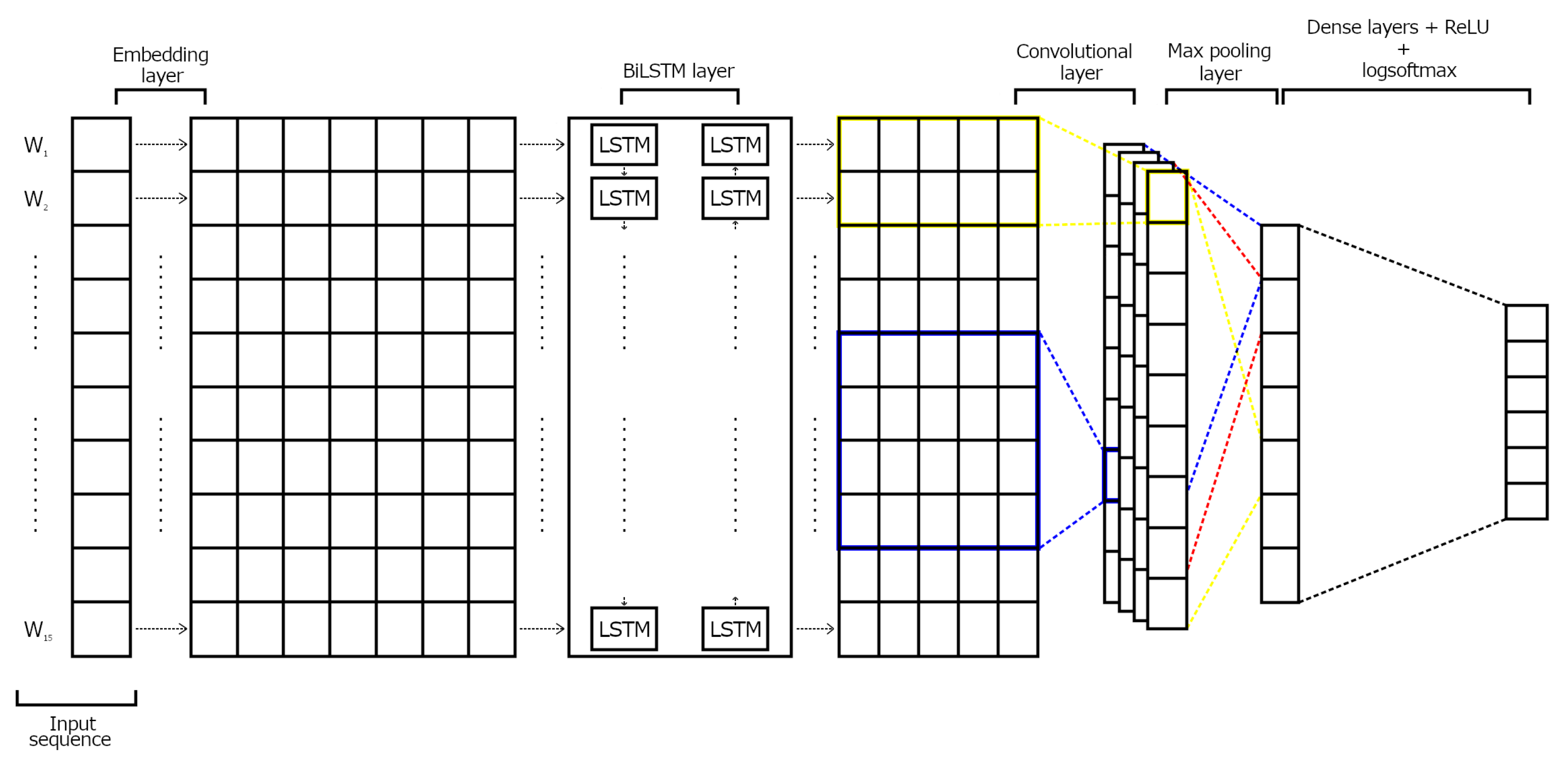
The main goal of this paper is to study both unimodal and multimodal approaches to deal with a finer-grained classification of fake news. To do this, we use the Fakeddit dataset [18], made up of posts from Reddit. The posts are classified into the following six different classes: true, misleading content, manipulated content, false connection, imposter content, and satire. We explore several deep learning architectures for text classification, such as Convolutional Neural Network (CNN) [19], Bidirectional Long Short-Term Memory (BiLSTM) [
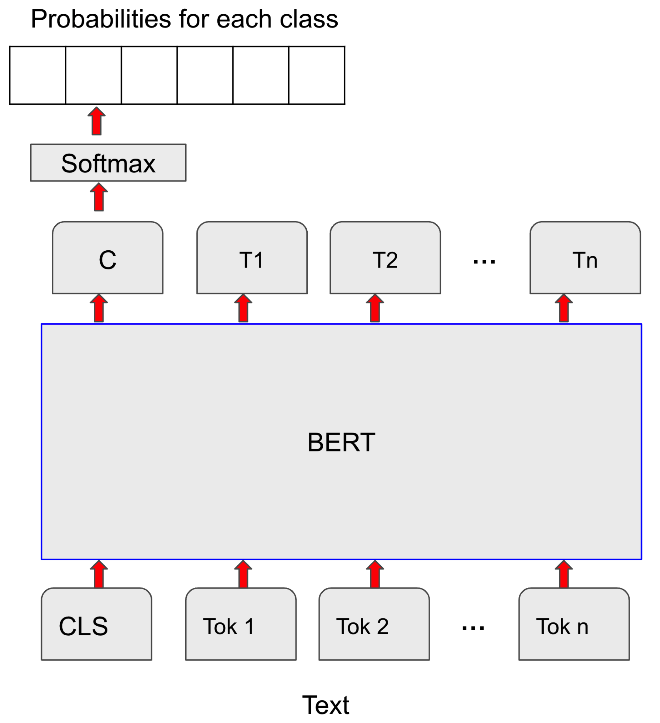
20], and Bidirectional Encoder Representations from Transformers (BERT) [21]. As a multimodal approach, we propose a CNN architecture that combines both texts and images to classify fake news.

3. Materials and Methods

In this section, we describe our approaches to dealing with the task of fake news detection. First, we present the unimodal approaches that only use texts. Then, we describe our multimodal approach, exploiting texts and images.

3.1. Dataset

In our experiments, we train and test our models using the Fakeddit dataset [18], which consists of a collection of posts from Reddit users. It includes texts, images, comments, and metadata. The texts are the titles of the posts submitted by users, while the comments are made by other users as an answer to a specific post. Thus, the dataset contains over 1 million instances.
One of the main advantages of this dataset is that it can be used to implement systems capable of performing a finer-grained classification of fake news than the usual binary classification, which only distinguishes between true and fake news. In the Fakeddit dataset, each instance has a label that distinguishes five categories of fake news, besides the unique category of true news. We briefly describe each category:
  • True: this category indicates that the news is true.
  • Manipulated Content: in this case, the content has been manipulated by different means (such as photo editing, for example).
  • False Connection: this category corresponds to those samples in which the text and the images are not in accordance.
  • Satire/Parody: this category refers to the news in which the meaning of the content is twisted or misinterpreted in a satirical or humorous way.
  • Misleading Content: this category corresponds to the news in which the information has been deliberately manipulated or altered in order to mislead the public.
  • Imposter Content: in the context of this project, all the news that belongs to this category include content generated by bots.
The Fakeddit dataset is divided into training, validation, and test partitions. Moreover, there are two different versions of the dataset: the unimodal dataset, whose instances only contains texts, and the multimodal dataset, whose instances have both text and image. The full dataset contains a total of 682,661 news with images. There are almost 290,000 additional texts without images. Therefore, 70% of the instances include both texts and images, while 30% only contain texts. Actually, all texts of the multimodal dataset are also included in the unimodal dataset.
Table 1 shows the distribution of the classes in the unimodal dataset. Table 2 provides the same information for the multimodal dataset. As we can see, all classes follow a similar distribution in both versions of the dataset (unimodal and multimodal) as well as in the training, validation, and test splits. Moreover, both datasets, unimodal and multimodal, are clearly imbalanced (the classes true, manipulated content, and false connection have more instances than the other classes satire, misleading content, and imposter content, which are much more underrepresented in both datasets). This imbalance may cause the classification task to be more difficult for those classes with fewer instances.
Table 1. Class distribution for the unimodal scenario.
Table 2. Class distribution for the multimodal scenario.

3.2. Methods

We now describe our approaches to deal with the task of fake news detection. First, we present the unimodal approaches that only use texts. Three models only using the texts are proposed: CNN, BiLSTM, and BERT. Then, we describe our multimodal approach, exploiting texts and images.
All texts were cleaned by removing stopwords, punctuations, numbers, and multiple spaces. Then, we split each text into tokens and we apply lemmatization. After lemmatization, we transform the texts into sequences of integers. This is performed first, by learning the vocabulary of the corpus and building a dictionary where each word is mapped to a different integer number. This dictionary is used to transform each text into a sequence of integers. Every non-zero entry in such a sequence corresponds to a word in the original text. The original order of the words in the text is respected.
As we need to feed the deep learning models with vectors of the same length, we pad and truncate the sequences of integers so that they have the same number of entries. This has the disadvantage that those vectors that are too long will be truncated, and some information will be lost. In order to select the length of the padded\truncated vectors, we computed the percentage of texts that are shorter than 10, 15, 20, and 25 tokens. We saw that 98% of the texts have less than 15 tokens.
Since the number of texts that will have to be truncated is very small (less than 2%), very little information is lost. Therefore, we selected 15 as the length of the vectors after padding and truncating.
Then, an embedding layer transforms each integer value from the input sequence into a vector of word embeddings. Thus, each text is represented as a sequence of word embeddings, which is the input of each deep learning model. In particular, every text is transformed into a matrix of 15 rows and 300 columns (300 being the dimension of the word embeddings).

3.2.1. CNN

We now explain the CNN architecture for the text classification of fake news. As was mentioned above, the first layer is an embedding layer. We initialize the embedding matrix using both random initialization and the pre-trained GloVe word embeddings of dimension 300. We chose this size for the word embeddings over other options (50, 100 or 200) because word embeddings of a larger dimension have been proven to give better results [60].
After the embedding layer, we apply four different filters in a convolutional layer. A convolutional operation is essentially the multiplication of the embedding matrix with a filter to extract the most representative features from the matrix. Each of these filters slides across the (15 × 300) matrix with the embeddings of the input sequence and generates 50 output channels. The 4 filters have sizes (2 × 300), (3 × 300), (4 × 300), and (5 × 300), respectively, since these are the typical filter sizes of a CNN for text classification [61]. As a consequence, the outputs of the previous filters have shapes (14 × 1), (13 × 1), (12 × 1), and (11 × 1), respectively.
The next step is to pass the outputs obtained from the previous layer through the ReLU activation function. This function is applied element-wise, and, therefore, it does not alter the size of the outputs obtained after the previous step. The effect of this function is to set all the negative values to 0 and leave the positive values unchanged.
To reduce the size of the model, after going through the ReLU activation, we will apply a maxpooling layer that selects the biggest element out of each of the 200 feature maps (50 feature maps per each of the 4 filters). Thus, 200 single numbers are generated.
These 200 numbers are concatenated, and the result is passed through 2 dense layers with 1 ReLU activation in between [24]. The resulting output is a vector of six entries (each entry corresponding to a different class of the Fakeddit dataset) that, after passing through the logsoftmax function, can be used to obtain the predicted class for the corresponding input text.
Early stopping [62] with the train and validation partitions is used in order to select the appropriate number of epochs. We use the Adam optimization algorithm [63] for training the model and the negative log-likelihood as the loss function.

3.2.2. BiLSTM + CNN

We now present a hybrid model that uses a bidirectional LSTM followed by a CNN layer. First, texts are processed as was described above, and these inputs are passed through the same embedding layer that was used for the CNN model. Therefore, each input vector of length 15 is transformed into a matrix of shape 15 × 300.
Then, the matrix with the word embeddings goes through a bidirectional LSTM layer with hidden states of length 70. The output of this layer is a matrix of size 15 × 140 that contains two hidden states (corresponding to the two directions of the BiLSTM) for each word embedding. The output of the BiLSTM layer is the input of a convolutional layer, which applies 240 filters of size (3 × 140). Therefore, it generates 240 output arrays of size (13 × 1). Then, the ReLU activation is applied, followed by a maxpooling layer that selects the largest element within each of the 240 feature maps. Thus, this layer outputs a sequence of 240 numbers.
Similar to what was done for the CNN model, the output of the maxpooling layer is concatenated and passed through two dense layers with ReLU activation in between. The resulting vector goes through the logsoftmax function, and the predicted class is obtained. Figure 1 shows the architecture of the BiLSTM for text classification.
Figure 1. BiLSTM + CNN for text classification.
Early stopping is again used for selecting the optimal number of epochs. We use Adam as the optimization algorithm and the negative log-likelihood as the loss function.

3.2.3. BERT

In this case, instead of using random initialization of the pre-trained Glove embeddings, we now use the vectors provided by BERT to represent the input tokens. As opposed to the GloVe model [64], BERT takes into account the context of each word (that is, the words that surround it).
For the preprocessing of the texts, the steps are similar to those described above. The main differences are that we tokenize the texts by using the BertTokenizer class from the transformers library [65]. This class has its own vocabulary with the mappings between words and ID, so it was not necessary to train a tokenizer with the corpus of texts. We also add the [CLS] and [SEP] tokens at the beginning and at the end of each tokenized sequence. It was also necessary to create an attention mask in order to distinguish what entries in each sequence correspond to real words in the input text and what entries are just 0 s resulting from padding the sequences. Thus, the attention mask is composed of 1 s (indicating non-padding entries) and 0 s (indicating padding entries). We use the BERT base model in its uncased version (12 layers, 768 hidden size, 12 heads, and 110 million parameters).
Then, we fine-tune it on our particular problem; that is, the multi-classification of fake news. To do this, we add a softmax layer on top of the output of BERT. The softmax layer receives a vector of length 768 and outputs a vector of length 6 (see Figure 2), which contains the probabilities for each class.
Figure 2. BERT for text classification.
For the training process, we used the Adam algorithm for optimization with a learning rate of 2 × 10 5 . We trained the model for two epochs since the authors of BERT recommended using between two and four epochs for fine-tuning on a specific NLP task [21].

3.2.4. Multimodal Approach

Our multimodal approach uses a CNN that takes both the text and the image corresponding to the same news as inputs. The model outputs a vector of six numbers, out of which the predicted class is obtained. In the following lines, we describe the preprocessing steps applied before feeding the data into the network, as well as the architecture of the network (see Figure 3).
Figure 3. Architecture of the multimodal approach for fake news detection.
Regarding the preprocessing of the images, we only reshaped them so that they all have the same shape (560 × 560). Once the preprocessed data are fed into the network, different operations are applied to the texts and images. We use the same CNN architecture that we have used for the unimodal scenario, except for the fact that we eliminate the last two dense layers with ReLU activation in between.
We now describe the CNN model to classify the images. The data first goes through a convolutional layer. Since each image is made up of three channels, the number of input channels of this layer is also three. Moreover, it has six output channels. Filters of size (5 × 5) are used with a stride equal to 1 and no padding. The output for each input image is, therefore, a collection of 6 matrices of shape (556 × 556). The output of the convolutional layer passes through a non-linear activation function (ReLU), and then maxpooling is applied with a filter of size (2 × 2) and a stride equal to 2. The resulting output is a set of six matrices of shape (278 × 278). The output from the maxpooling layer again passes through another convolutional layer that has 6 input channels and 3 output channels. The filter size, stride length, and padding are the same as those used in the previous convolutional layer. Then, the ReLU non-linear activation function and the maxpooling layer are applied again over the feature maps resulting from the convolutional layer. Thus, for a given input (image), we obtain a set of 3 feature maps of shape (137 × 137). Finally, these feature maps are flattened into a vector of length 56,307.
The texts are also processed by using the same CNN model for texts, which was described previously. However, instead of feeding the output of the dense layer to the softmax layer in the CNN model, this output vector representing the text is concatenated to the vector obtained by the CNN model for images. Then, this vector is passed through two dense layers with a ReLU non-linear activation in between. Finally, the logsoftmax function is applied, and the logarithm of the probabilities is used in order to compute the predicted class of the given input.

4. Results

In this section, we present the results obtained for each model. We report the recall, precision, and F1 scores obtained by all the models for each class. The accuracy is computed over all the classes. It helps us to compare models and find the best approach. Moreover, we are also interested in knowing which model is better at detecting only those news containing false content. For this reason, we also compute the micro and macro averages of the recall, precision, and F1 metrics only over five classes of fake news without the true news. Macro averaging computes the metrics for each class and then calculates the average. Micro averaging calculated the sum of all true positives and false positives for all the classes, and then computes the metrics. We use the F 1 m i c r o score and the accuracy to compare the performance of the models.

4.1. CNN Results

Our first experiment with CNN uses random initialization to initialize the weights of the embedding layer, which are updated during the training process. This model obtains an accuracy of 72%, a micro F1 of 57%, and a macro F1 of 49% (see Table 3). We can also see that True and Manipulated content are the classes with the highest F1 (79%). A possible reason for this could be that they are the majority classes. On the other hand, the model obtains the lowest F1 (13%) for Imposter content, which is the minority class in the dataset (see Table 1). Therefore, the results for the different classes appear to be related to the number of instances per class. However, the model achieves an F1 of 61% for the second minority class, Misleading content. As was explained before, the content of this news has been deliberately manipulated. Identifying these manipulations appears to be easier than detecting humor or sarcasm in the news (Satire) or fake news generated by bots (Imposter content).
Table 3. Results of CNN with random initialization.
Interestingly, although the model only exploits the textual content of the news, it achieves an F1 of 57% for classifying the instances of False connections. In these instances, the text and the image are not in accordance.
We also explore CNN with static (see Table 4) and dynamic (see Table 5) GloVe embeddings [64]. In both models, the embedding layer is initialized with the pre-trained Glove vectors. When dynamic training is chosen, these vectors are updated during the training process. On the other hand, if static training is chosen, the vectors are fixed during the training process. The model with dynamic vectors overcomes the one with static vectors, with a slight improvement in accuracy (74%) (roughly one percentage point). However, in terms of micro F1, the static model is better than the dynamic one. Both models provide the same macro F1 (69%). Regarding the classes, there are no significant differences, except for Imposer content. For this class, updating the pre-trained Glove vectors results in a decrease of seven percentage points in F1.
Table 4. Results of CNN with static Glove vectors.
Table 5. Results of CNN with dynamic Glove vectors.
We also compared the effect of the pre-trained Glove vectors with random initialization (see Table 3). In both dynamic and static approaches, initializing the model with the pre-trained GloVe word embeddings gets better results than random initialization. The reason for this is that the GloVe vectors contain information about the relationship between different words that random vectors can not capture.
As the dataset is highly unbalanced, we use the micro F1 to assess and compare the overall performances of the three models. Thus, the best model is a CNN with dynamic Glove vectors. However, dynamic training takes much more time than static training (around 6000 to 8000 s more). This is due to the fact that, in a dynamic approach, word embeddings are also learned, and this significantly increases the training time.

4.2. BiLSTM + CNN Results

As a second deep learning model, we explore a hybrid model based on a BiLSTM followed by a CNN. We replicate the same experiments as described for CNN; that is, using random initialization and pre-trained Glove vectors.
The BiLSTM initialized with random vectors (see Table 6) very similar results to those achieved by CNN with random initialization (see Table 3). In fact, both models provide the same accuracy of 0.72. However, in terms of micro F1, the BiLSTM model obtains up to nine points more than the CNN model with random initialization. This improvement may be because the BiLSTM improved its scores for Imposter content.
Table 6. Results of BiLSTM with random initialization.
The use of static Glove vectors (see Table 7) appears to have a positive effect on the performance of the BiLSTM model. The model shows significant improvements for False connection, Satire, Misleading content, and Imposter content, with increases of 6, 12, 3, and 10 points, respectively. The model obtains an accuracy of 73%. Therefore, the pre-trained Glove vectors achieve better results than random initialization.
Table 7. Results of BiLSTM with static Glove vectors.
Table 8 shows the results obtained by BiLSTM with dynamic Glove vectors. If these vectors are updated during the training of the BiLSTM model, an accuracy of 75% is achieved; that is, two points more than BiLSTM with static Glove vectors. Moreover, this model with dynamic Glove vectors improves the results for all classes, with increases ranging from one to four points. In terms of micro F1, using dynamic Glove vectors is the best approach for BiLSTM. Moreover, this model slightly overcomes the CNN model with dynamic Glove vectors by roughly one percentage point. However, as mentioned above, dynamic training takes much more time than static training.
Table 8. Results of BiLSTM with dynamic Glove vectors.

4.3. Bert Results

Table 9 shows the results obtained by BERT. This model achieves an accuracy of 78% and a micro F1 of 74%. Therefore, it outperforms all the previous unimodal deep learning approaches. This proves the advantage of the pre-trained contextual text representations provided by BERT, as opposed to the context-free GloVe vectors or random initialization for neural networks.
Table 9. BERT results.
Moreover, BERT is better in all classes. Comparing the classes, the behavior of BERT is very similar to the previous deep learning models; that is, the more training instances for a class, the better predictions for it. In this way, True and Manipulated content both get the highest F1 (83%), while the worst-performing class is Imposter content (F1 = 38%). As in previous models, Misleading content gets better scores than Satire, despite the fact that this class is more represented than the first one, Misleading content (see Table 2).

4.4. Multimodal Approach Results

The multimodal approach obtains an accuracy of 87% and a micro F1 of 72% (see Table 10), which are the highest scores out of all the unimodal models.
Table 10. Multimodal approach results.
As expected, the training set size for each class strongly affects the model scores. While True and Manipulated content, the majority classes, get the highest scores, Imposter content, the minority class, shows the lowest F1 (32%), even six points lower than that provided by BERT for the same class (F1 = 38%). Thus, we can say that the image content provides little information for identifying instances of Imposter content. Manipulated content shows an F1 of 100%. This is probably due to the fact that the images in this category have been manipulated. These manipulations may be easily detected by CNN.
As expected, the use of images significantly improves the results for False connection. The multimodal model shows an F1 of 76%, 8 points higher than that obtained by BERT, the best unimodal approach, and 15 points higher than the unimodal CNN model using only texts. The improvement is even greater for detecting instances of Satire, with an increase of 16 points higher than those obtained by BERT and by the unimodal CNN model.

5. Discussion

In addition to the deep learning algorithms, we also propose a Support Vector Machine (SVM) as a baseline for the unimodal approaches. SVM is one of the most successful algorithms for text classification. For this algorithm, the texts were represented using the tf-idf model. Table 11 shows a comparison of the best models (traditional algorithms, CNN, BiLSTM, BERT, and multimodal CNN) according to their accuracy and micro average scores.
Table 11. Comparison of the best models (micro_averages).
We can see that the multimodal CNN outperforms all the unimodal approaches. In fact, the multimodal approach achieves higher accuracy than that provided by the best model of the unimodal approaches, BERT, with a difference of 9% in overall accuracy. In terms of micro-F1, the improvement is even greater, 13 points over the micro F1 of BERT. This proves the usefulness of combining texts and images for a fine-grained fake news classification.
Focusing on the unimodal approaches, the BERT model is the best both in terms of accuracy and micro F1 score, which shows the advantage of using contextual word embeddings. In terms of accuracy, BERT achieves a significant improvement over the other deep learning models. The third best approach is BiLSTM + CNN with dynamic Glove vectors, with an accuracy of 0.75 (three points lower than the accuracy achieved by BERT). The fourth approach is the CNN model, with an accuracy of 0.74 (four points lower than the accuracy provided by BERT). In terms of micro F1, BERT also outperforms the other deep learning models, with improvements of around 4–5%. Finally, all the deep learning approaches outperform our baseline SVM, with an accuracy of 0.72. This also shows that when a large dataset is available, as in the case of the Fakeddit dataset, the deep learning models provide better performance than traditional machine learning algorithms.

6. Conclusions

Fake news could have a significant negative effect on politics, health, and economies. Therefore, it becomes necessary to develop tools that allow for the rapid and reliable detection of misinformation.
Apart from the work carried out by the creators of the Fakeddit dataset [18], this is, to the best of our knowledge, the only study that addresses a fine-grained classification of fake news by performing a comprehensive comparison of unimodal and multimodal approaches based on the most advanced deep learning techniques.
The multimodal approach overcomes the approaches that only exploit texts. BERT is the best model for the task of text classification. Moreover, using dynamic GloVe word embeddings outperforms random initialization for the CNN and BiLSTM architectures.
In future work, we plan to use pre-trained networks to generate the visual representations. In particular, we will use the network VGG, which was pre-trained on a large dataset of images, such as ImageNet. We also plan to explore different deep learning techniques, such as LSTM, BiLSTM, GRU, or BERT, as well as different methods of combining the visual and textual representations. In our current study, we have built our multimodal CNN using an early fusion approach, which consists of creating textual and visual representations, combining them, and then applying a classifier over the resulting combined representation to get the probabilities for each class. Instead of this, we plan to study a late fusion approach, which would require two separate classifiers (one for the textual inputs and the other for the image inputs). The predictions from both classifiers are then combined, and the final prediction is obtained.

Author Contributions

Conceptualization, I.S.-B. and S.A.-B.; methodology, I.S.-B.; software, S.A.-B.; validation, I.S.-B. and S.A.-B.; formal analysis, I.S.-B.; investigation, I.S.-B.; writing—original draft preparation, I.S.-B. and S.A.-B.; writing—review and editing, I.S.-B.; supervision, I.S.-B.; project administration, I.S.-B.; funding acquisition, I.S.-B. All authors have read and agreed to the published version of the manuscript.

Funding

This research was funded by the Madrid Government (Comunidad de Madrid) under the Multiannual Agreement with UC3M in the line of “Fostering Young Doctors Research” (NLP4RARE-CM-UC3M) and in the context of the V PRICIT (Regional Programme of Research and Technological Innovation) and under the Multiannual Agreement with UC3M in the line of Excellence of University Professors (EPUC3M17).

Institutional Review Board Statement

Not applicable.

Data Availability Statement

The source code is available from https://github.com/isegura/MultimodalFakeNewsDetection (accessed on 1 June 2022).

Conflicts of Interest

The authors declare no conflict of interest.

Abbreviations

The following abbreviations are used in this manuscript:
BERTBidirectional Encoder Representations from Transformer
BiLSTMBidirectional Long Short-Term Memory
CNNConvolutional Neural Network
NLPNatural Language Processing
SVMSupport Vector Machine

References

  1. Finneman, T.; Thomas, R.J. A family of falsehoods: Deception, media hoaxes and fake news. Newsp. Res. J. 2018, 39, 350–361. [Google Scholar] [CrossRef]
  2. Hunt, A.; Gentzkow, M. Social Media and Fake News in the 2016 Election. J. Econ. Perspect. 2017, 31, 211–236. [Google Scholar] [CrossRef] [Green Version]
  3. Hauck, G. Pizzagate Shooter Sentenced to 4 Years in Prison. CNN. 2017. Available online: https://edition.cnn.com/2017/06/22/politics/pizzagate-sentencing/index.html (accessed on 1 June 2022).
  4. Mishra, V. India’s Fake News Problem is Killing Real People. Asia Times. 2019. Available online: https://asiatimes.com/2019/10/indias-fake-news-problem-is-killing-real-people/ (accessed on 1 June 2022).
  5. Greene, C.M.; Murphy, G. Quantifying the effects of fake news on Behavior: Evidence from a study of COVID-19 misinformation. J. Exp. Psychol. Appl. 2021, 27, 773–784. [Google Scholar] [CrossRef] [PubMed]
  6. Islam, M.; Kamal, A.H.; Kabir, A.; Southern, D.; Khan, S.; Hasan, S.; Sarkar, T.; Sharmin, S.; Das, S.; Roy, T.; et al. COVID-19 vaccine rumors and conspiracy theories: The need for cognitive inoculation against misinformation to improve vaccine adherence. PLoS ONE 2021, 16, e0251605. [Google Scholar] [CrossRef] [PubMed]
  7. Brown, E. Online Fake News is Costing us $78 Billion Globally Each Year. ZDNet. 2019. Available online: https://www.zdnet.com/article/online-fake-news-costing-us-78-billion-globally-each-year/ (accessed on 1 June 2022).
  8. Thota, A.; Tilak, P.; Ahluwalia, S.; Lohia, N. Fake news detection: A deep learning approach. SMU Data Sci. Rev. 2018, 1, 10. [Google Scholar]
  9. Choudhary, M.; Chouhan, S.S.; Pilli, E.S.; Vipparthi, S.K. BerConvoNet: A deep learning framework for fake news classification. Appl. Soft Comput. 2021, 110, 107614. [Google Scholar] [CrossRef]
  10. Singh, V.K.; Ghosh, I.; Sonagara, D. Detecting fake news stories via multimodal analysis. J. Assoc. Inf. Sci. Technol. 2021, 72, 3–17. [Google Scholar] [CrossRef]
  11. Giachanou, A.; Zhang, G.; Rosso, P. Multimodal multi-image fake news detection. In Proceedings of the 2020 IEEE 7th International Conference on Data Science and Advanced Analytics (DSAA), Sydney, Australia, 6–9 October 2020; pp. 647–654. [Google Scholar]
  12. Singhal, S.; Shah, R.R.; Chakraborty, T.; Kumaraguru, P.; Satoh, S. SpotFake: A multi-modal framework for fake news detection. In Proceedings of the 2019 IEEE Fifth International Conference on Multimedia Big Data (BigMM), Singapore, 11–13 September 2019; pp. 39–47. [Google Scholar]
  13. Wang, Y.; Ma, F.; Jin, Z.; Yuan, Y.; Xun, G.; Jha, K.; Su, L.; Gao, J. EANN: Event adversarial neural networks for multi-modal fake news detection. In Proceedings of the 24th ACM SIGKDD International Conference on Knowledge Discovery & Data Mining, London, UK, 19–23 August 2018; pp. 849–857. [Google Scholar]
  14. Parcalabescu, L.; Trost, N.; Frank, A. What is Multimodality? In Proceedings of the 1st Workshop on Multimodal Semantic Representations (MMSR), Online, 14–18 June 2021; pp. 1–10. [Google Scholar]
  15. Kiela, D.; Firooz, H.; Mohan, A.; Goswami, V.; Singh, A.; Ringshia, P.; Testuggine, D. The hateful memes challenge: Detecting hate speech in multimodal memes. Adv. Neural Inf. Process. Syst. 2020, 33, 2611–2624. [Google Scholar]
  16. Radford, A.; Kim, J.W.; Hallacy, C.; Ramesh, A.; Goh, G.; Agarwal, S.; Sastry, G.; Askell, A.; Mishkin, P.; Clark, J.; et al. Learning transferable visual models from natural language supervision. In Proceedings of the International Conference on Machine Learning. PMLR, Virtual Event, 13–14 August 2021; pp. 8748–8763. [Google Scholar]
  17. Kumari, R.; Ekbal, A. AMFB: Attention based multimodal Factorized Bilinear Pooling for multimodal Fake News Detection. Expert Syst. Appl. 2021, 184, 115412. [Google Scholar] [CrossRef]
  18. Nakamura, K.; Levy, S.; Wang, W.Y. Fakeddit: A New Multimodal Benchmark Dataset for Fine-grained Fake News Detection. In Proceedings of the 12th Language Resources and Evaluation Conference, Marseille, France, 21–23 June 2020; European Language Resources Association: Marseille, France, 2020; pp. 6149–6157. [Google Scholar]
  19. Goodfellow, I.; Bengio, Y.; Courville, A. Convolutional Networks. In Deep Learning; MIT Press: Cambridge, MA, USA, 2016; pp. 321–362. [Google Scholar]
  20. Hochreiter, S.; Schmidhuber, J. Long Short-Term Memory. Neural Comput. 1997, 9, 1735–1780. [Google Scholar] [CrossRef]
  21. Devlin, J.; Chang, M.W.; Lee, K.; Toutanova, K. Bert: Pre-training of deep bidirectional transformers for language understanding. In Proceedings of the NAACL-HLT 2019, Minneapolis, MN, USA, 2–7 June 2019; pp. 4171–4186. [Google Scholar]
  22. O’Mahony, N.; Campbell, S.; Carvalho, A.; Harapanahalli, S.; Hernandez, G.V.; Krpalkova, L.; Riordan, D.; Walsh, J. Deep learning vs. traditional computer vision. In Proceedings of the Science and Information Conference, Leipzig, Germany, 1–4 September 2019; pp. 128–144. [Google Scholar]
  23. Deng, L.; Liu, Y. Deep Learning in Natural Language Processing, 1st ed.; Springer: Berlin/Heidelberg, Germany, 2018. [Google Scholar]
  24. Minaee, S.; Kalchbrenner, N.; Cambria, E.; Nikzad, N.; Chenaghlu, M.; Gao, J. Deep Learning–based Text Classification: A Comprehensive Review. ACM Comput. Surv. (CSUR) 2021, 54, 1–40. [Google Scholar] [CrossRef]
  25. Abavisani, M.; Wu, L.; Hu, S.; Tetreault, J.; Jaimes, A. Multimodal Categorization of Crisis Events in Social Media. In Proceedings of the 2020 IEEE/CVF Conference on Computer Vision and Pattern Recognition (CVPR), Seattle, WA, USA, 13–19 June 2020; IEEE Computer Society: Los Alamitos, CA, USA, 2020; pp. 14667–14677. [Google Scholar]
  26. Bae, K.I.; Park, J.; Lee, J.; Lee, Y.; Lim, C. Flower classification with modified multimodal convolutional neural networks. Expert Syst. Appl. 2020, 159, 113455. [Google Scholar] [CrossRef]
  27. Yu, J.; Jiang, J. Adapting BERT for Target-Oriented Multimodal Sentiment Classification. In Proceedings of the Twenty-Eighth International Joint Conference on Artificial Intelligence, IJCAI-19, Macao, China, 10–16 August 2019; pp. 5408–5414. [Google Scholar]
  28. Viana, M.; Nguyen, Q.B.; Smith, J.; Gabrani, M. Multimodal Classification of Document Embedded Images. In Proceedings of the International Workshop on Graphics Recognition, Nancy, France, 22–23 August 2017; pp. 45–53. [Google Scholar]
  29. Gaspar, A.; Alexandre, L.A. A multimodal approach to image sentiment analysis. In Proceedings of the International Conference on Intelligent Data Engineering and Automated Learning, Manchester, UK, 14–16 November 2019; Springer: Cham, Switzerland, 2019; pp. 302–309. [Google Scholar]
  30. Baheti, P. Introduction to Multimodal Deep Learning. 2020. Available online: https://heartbeat.comet.ml/introduction-to-multimodal-deep-learning-630b259f9291 (accessed on 13 November 2021).
  31. Wani, A.; Joshi, I.; Khandve, S.; Wagh, V.; Joshi, R. Evaluating deep learning approaches for COVID-19 fake news detection. In Proceedings of the Combating Online Hostile Posts in Regional Languages during Emergency Situation: First International Workshop, CONSTRAINT 2021, Collocated with AAAI 2021, Virtual Event, 8 February 2021; p. 153. [Google Scholar]
  32. Patwa, P.; Sharma, S.; Pykl, S.; Guptha, V.; Kumari, G.; Akhtar, M.S.; Ekbal, A.; Das, A.; Chakraborty, T. Fighting an infodemic: COVID-19 fake news dataset. arXiv 2020, arXiv:2011.03327. [Google Scholar]
  33. Yang, Z.; Yang, D.; Dyer, C.; He, X.; Smola, A.; Hovy, E. Hierarchical attention networks for document classification. In Proceedings of the 2016 Conference of the North American Chapter of the Association for Computational Linguistics: Human Language Technologies, San Diego, CA, USA, 12–17 June 2016; pp. 1480–1489. [Google Scholar]
  34. Sanh, V.; Debut, L.; Chaumond, J.; Wolf, T. DistilBERT, a distilled version of BERT: Smaller, faster, cheaper and lighter. arXiv 2019, arXiv:1910.01108. [Google Scholar]
  35. Goldani, M.H.; Momtazi, S.; Safabakhsh, R. Detecting fake news with capsule neural networks. Appl. Soft Comput. 2021, 101, 106991. [Google Scholar] [CrossRef]
  36. Sabour, S.; Frosst, N.; Hinton, G.E. Dynamic routing between capsules. arXiv 2017, arXiv:1710.09829. [Google Scholar]
  37. Ahmed, H.; Traore, I.; Saad, S. Detection of online fake news using n-gram analysis and machine learning techniques. In Proceedings of the International Conference on Intelligent, Secure, and Dependable Systems in Distributed and Cloud Environments, Vancouver, BC, Canada, 26–28 October 2017; pp. 127–138. [Google Scholar]
  38. Wang, W.Y. “Liar, Liar Pants on Fire”: A new benchmark dataset for fake news detection. arXiv 2017, arXiv:1705.00648. [Google Scholar]
  39. Girgis, S.; Amer, E.; Gadallah, M. Deep Learning Algorithms for Detecting Fake News in Online Text. In Proceedings of the 2018 13th International Conference on Computer Engineering and Systems (ICCES), Cairo, Egypt, 18–19 December 2018; pp. 93–97. [Google Scholar] [CrossRef]
  40. Aggarwal, C.C. Recurrent Neural Networks. In Neural Networks and Deep Learning: A Textbook; Springer International Publishing: Cham, Switzerland, 2018; pp. 271–313. [Google Scholar]
  41. Chung, J.; Gulcehre, C.; Cho, K.; Bengio, Y. Empirical evaluation of gated recurrent neural networks on sequence modeling. arXiv 2014, arXiv:1412.3555. [Google Scholar]
  42. Kleinbaum, D.G.; Klein, M. Logistic Regression, 3rd ed.; Springer: New York, NY, USA, 2010. [Google Scholar]
  43. Hastie, T.; Tibshirani, R.; Friedman, J. Additive Models, Trees, and Related Methods. In The Elements of Statistical Learning: Data Mining, Inference, and Prediction; Springer: New York, NY, USA, 2009; pp. 295–336. [Google Scholar]
  44. Murphy, K. Kernels. In Machine Learning: A Probabilistic Perspective; The MIT Press: Cambridge, MA, USA, 2012; pp. 479–512. [Google Scholar]
  45. Barber, D. Naive Bayes. In Bayesian Reasoning and Machine Learning; Cambridge University Press: Cambridge, UK, 2012; pp. 243–255. [Google Scholar] [CrossRef] [Green Version]
  46. Hastie, T.; Tibshirani, R.; Friedman, J. Support Vector Machines and Flexible Discriminants. In The Elements of Statistical Learning: Data Mining, Inference, and Prediction; Springer: New York, NY, USA, 2009; pp. 417–458. [Google Scholar] [CrossRef]
  47. Breiman, L. Random Forests. Mach. Learn. 2001, 45, 5–32. [Google Scholar] [CrossRef] [Green Version]
  48. Kaggle. Getting Real about Fake News. Available online: https://www.kaggle.com/mrisdal/fake-news (accessed on 13 October 2021).
  49. Simonyan, K.; Zisserman, A. Very deep convolutional networks for large-scale image recognition. arXiv 2014, arXiv:1409.1556. [Google Scholar]
  50. Shu, K.; Mahudeswaran, D.; Wang, S.; Lee, D.; Liu, H. FakeNewsNet: A Data Repository with News Content, Social Context, and Spatiotemporal Information for Studying Fake News on Social Media. Big Data 2020, 8, 171–188. [Google Scholar] [CrossRef] [PubMed]
  51. Boididou, C.; Andreadou, K.; Papadopoulos, S.; Dang-Nguyen, D.T.; Boato, G.; Riegler, M.; Kompatsiaris, Y. Verifying Multimedia Use at MediaEval 2015. MediaEval 2015, 3, 7. [Google Scholar]
  52. Jin, Z.; Cao, J.; Guo, H.; Zhang, Y.; Luo, J. Multimodal fusion with recurrent neural networks for rumor detection on microblogs. In Proceedings of the 25th ACM international conference on Multimedia, Mountain View, CA, USA, 23–27 October 2017; pp. 795–816. [Google Scholar]
  53. Kaliyar, R.K.; Kumar, P.; Kumar, M.; Narkhede, M.; Namboodiri, S.; Mishra, S. DeepNet: An Efficient Neural Network for Fake News Detection using News-User Engagements. In Proceedings of the 2020 5th International Conference on Computing, Communication and Security (ICCCS), Patna, India, 14–16 October 2020; pp. 1–6. [Google Scholar] [CrossRef]
  54. Kaggle. FakeNewsNet. Available online: https://www.kaggle.com/mdepak/fakenewsnet (accessed on 14 October 2021).
  55. Kirchknopf, A.; Slijepcevic, D.; Zeppelzauer, M. Multimodal Detection of Information Disorder from Social Media. arXiv 2021, arXiv:2105.15165. [Google Scholar]
  56. Li, P.; Sun, X.; Yu, H.; Tian, Y.; Yao, F.; Xu, G. Entity-Oriented Multi-Modal Alignment and Fusion Network for Fake News Detection. IEEE Trans. Multimed. 2021, 99, 1. [Google Scholar] [CrossRef]
  57. Xie, J.; Liu, S.; Liu, R.; Zhang, Y.; Zhu, Y. SERN: Stance Extraction and Reasoning Network for Fake News Detection. In Proceedings of the ICASSP 2021—2021 IEEE International Conference on Acoustics, Speech and Signal Processing (ICASSP), Virtual Conference, 6–12 June 2021; pp. 2520–2524. [Google Scholar] [CrossRef]
  58. Zubiaga, A.; Liakata, M.; Procter, R. Exploiting context for rumour detection in social media. In Proceedings of the International Conference on Social Informatics, Oxford, UK, 13–15 September 2017; pp. 109–123. [Google Scholar]
  59. Kang, Z.; Cao, Y.; Shang, Y.; Liang, T.; Tang, H.; Tong, L. Fake News Detection with Heterogenous Deep Graph Convolutional Network. In Proceedings of the Advances in Knowledge Discovery and Data Mining, Virtual Event, 11–14 May 2021; Karlapalem, K., Cheng, H., Ramakrishnan, N., Agrawal, R.K., Reddy, P.K., Srivastava, J., Chakraborty, T., Eds.; Springer International Publishing: Cham, Switzerland, 2021; pp. 408–420. [Google Scholar]
  60. Patel, K.; Bhattacharyya, P. Towards lower bounds on number of dimensions for word embeddings. In Proceedings of the Eighth International Joint Conference on Natural Language Processing, Taipei, Taiwan, 27 November–1 December 2017; pp. 31–36. [Google Scholar]
  61. Voita, E. Convolutional Neural Networks for Text. 2021. Available online: https://lena-voita.github.io/nlp_course/models/convolutional.html (accessed on 5 October 2021).
  62. Brownlee, J. A Gentle Introduction to Early Stopping to Avoid Overtraining Neural Networks. Available online: https://machinelearningmastery.com/early-stopping-to-avoid-overtraining-neural-network-models/ (accessed on 5 October 2021).
  63. Kingma, D.P.; Ba, J. Adam: A method for stochastic optimization. arXiv 2014, arXiv:1412.6980. [Google Scholar]
  64. Pennington, J.; Socher, R.; Manning, C.D. Glove: Global vectors for word representation. In Proceedings of the 2014 Conference on Empirical Methods in Natural Language Processing (EMNLP), Doha, Qatar, 25–29 October 2014; pp. 1532–1543. [Google Scholar]
  65. Face, H. Transformers. Available online: https://huggingface.co/transformers/ (accessed on 5 October 2021).
Publisher’s Note: MDPI stays neutral with regard to jurisdictional claims in published maps and institutional affiliations.

Article Metrics

Citations

Article Access Statistics

Multiple requests from the same IP address are counted as one view.