Article

Fast Tracking Algorithm Based on Spatial Regularization Correlation Filter

College of Information Science and Engineering, Xinjiang University, Urumqi 830046, China
*
Author to whom correspondence should be addressed.
Information 2022, 13(4), 184; https://doi.org/10.3390/info13040184
Submission received: 27 February 2022 / Revised: 25 March 2022 / Accepted: 30 March 2022 / Published: 2 April 2022

Abstract

:
To solve the problem of the redundant number of training samples in a correlation filter-based tracking algorithm, the training samples were implicitly extended by circular shifts of the given target patches, and all the extended samples were used as negative samples for the fast online learning of the filter. Since all these shifted patches were not true negative samples of the target, the tracking process suffered from boundary effects, especially in challenging situations such as occlusion and background clutter, which can significantly impair the tracking performance of the tracker. Spatial regularization in the SRDCF tracking algorithm is an effective way to mitigate boundary effects, but it comes at the cost of highly increased time complexity, resulting in a very slow tracking speed of the SRDCF algorithm that cannot achieve a real-time tracking effect. To address this issue, we proposed a fast-tracking algorithm based on spatially regularized correlation filters that efficiently optimized the solved filters by replacing the Gauss–Seidel method in the SRDCF algorithm with the alternating direction multiplier method. The problem of slow speed in the SRDCF tracking algorithm improved, and the improved FSRCF algorithm achieved real-time tracking. An adaptive update mechanism was proposed by using the feedback from the high confidence tracking results to avoid model corruption. That is, a robust confidence evaluation criterion was introduced in the model update phase, which combined the maximum response criterion and the average peak correlation energy APCE criterion to determine whether to update the filter, thereby avoiding filter model drift and improving the target tracking accuracy and speed. We conducted extensive experiments on datasets OTB-2015, OTB-2013, UAV123, and TC128, and the experimental results show that the proposed algorithm exhibits a more stable and accurate tracking performance in the presence of occlusion and background clutter during tracking.

1. Introduction

The field of computer vision contains many kinds of technical studies for different application scenarios. The typical application areas include video surveillance [1], unmanned driving [2], human–computer interaction [3], intelligent robots [4], and drone precision strikes [5], amongst others. The studies on tracking algorithms in the literature [6,7,8,9] show that target tracking has always occupied an important position in the field of computer vision. The target tracking process is to annotate the physical location of an object in a continuous sequence of video images, and eventually connect the target objects in consecutive frames to form a target motion trajectory path. It is essentially based on the given target image, using feature extraction and feature association techniques to match the features most likely to belong to the same target in different frames, and then connect the matched targets in consecutive frames to obtain the target’s motion trajectory and finally achieve the task of target tracking.
The correlation filter-based tracking algorithm uses a large number of cyclically shifted samples for learning and converts the correlation operation in the spatial domain into element multiplication in the frequency domain. This reduces the computational complexity and significantly improves the tracking speed. The MOSSE tracker [10] was the pioneer of the correlation filter algorithm, and its tracking speed can reach about 700 frames per second. The CSK tracker [11] proposed cyclic shifting for dense sampling based on the MOSSE tracker, and the later KCF tracker [12] also introduced cyclic shifting to generate training samples. Although the use of circular shift solves the problem of redundancy in the number of training samples, it also brings the problem of boundary effect. This is because the training samples it generates contain periodic repetition of image blocks that leads to inaccurate representation of parts of the input images, and inaccurate negative training image blocks reduce the discriminative power of the learned model.
In 2015, Danelljan’s team proposed the SRDCF model [13] for the boundary effect problem of the KCF algorithm. This model not only suppressed the background response and expanded the search region, but also proposed a regularization component to correlate the filters to solve the circular boundary effect problem. As the inclusion of the regularization component in the SRDCF model destroyed the closed solution of the standard discriminant correlation filter, the filter cannot be solved directly, so a Gauss–Seidel solver was used to solve the filter iteratively. However, the iteration speed of the Gauss–Seidel solver is too slow, resulting in a tracking speed of only 5 frames per second in this model, which does not meet the requirement of real-time target tracking.
In order to improve the accuracy and speed of SRDCF model tracking, and then achieve real-time target tracking, we proposed a fast-tracking algorithm based on a spatially regularized correlation filter, and the main contributions of this paper are summarized below.
First: We used the alternate direction method of multipliers (ADMM) [14] solver to replace the Gauss–Seidel solver in the process of solving the filter, which improved the overall target tracking speed by increasing the computational speed of solving the filter.
Second: In the model update phase we not only utilized the maximum response value, but also incorporated the average peak correlation energy (APCE) criterion [15], which indicated the degree of fluctuation on the response map and the confidence level of the detected targets. The fusion of these two criteria improved the accuracy of target tracking, and to some extent, also improved the speed of target tracking.
Third: We evaluated the proposed tracking algorithm using tests on the datasets OTB-2015, OTB-2013, UAV123, and TC128, and the experimental results show that the proposed algorithm exhibits a more stable and accurate tracking performance in the presence of occlusion and background clutter during tracking.

2. Related Work

2.1. Correlation Filtering

The correlation filter-based algorithm was first introduced in 2010 in the MOSSE tracker [10] proposed by Bolme et al. This tracker gives the first frame target region, either manually or conditionally, and then the features are extracted from this region and then fast Fourier transform (FFT) [16] operation is conducted. The results are multiplied with the correlation filter in the frequency domain, and then the inverse fast Fourier transform (IFFT) operation is conducted to obtain the output response points, including the maximum response point that is the target position of that frame. Finally, the frame target region is added to the training samples and the correlation filter is updated. In 2012, based on the MOSSE algorithm, Henriques et al. proposed the CSK algorithm [11], which used a circular matrix to increase the number of training samples and solved the problem of sample redundancy caused by sparse sampling in the traditional algorithm. In the same year, Danelljan et al. proposed the correlation filter CCSK [17] by adding color name features [17,18] to the CSK algorithm, which improved the characterization of sample information and, thus, the robustness of the tracker. In 2014, Danelljan et al. proposed the DSST model [19] for the problem of scale variation [20] in the field of target tracking. The fDSST [21] algorithm used feature dimensionality reduction to further accelerate the DSST algorithm, achieving a joint improvement in speed and performance. In 2015, Li et al. proposed the SAMF model [22], which used a kernel function approach to consider scale variation while incorporating grayscale features, color features, and histogram of oriented gradients (HOG) [23,24] features for target feature extraction. The powerful target feature information improved the robustness of the target tracking model to some extent. The 2015 kernel correlation filter (KCF) [12] further improved the CSK [11] algorithm by using multichannel HOG features and introduced the cyclic shift generation of training samples in the KCF tracker. The cyclic shift generation of training samples yielded a cyclic data matrix, and the cyclic data matrix was diagonalized using the discrete Fournier transform (DFT) operation for fast computation, thereby reducing the computational effort of the algorithm. Although the circular shift increased the number of training samples to a certain extent, it also introduced the boundary effect problem. The boundary effect problem makes the detection response values of the tracked target accurate only in and around the center of the target, while the rest of the detection response values are not referenced by the periodic repetition of the training samples, resulting in a very limited target search area during the detection process. In 2015, Danelljan’s team proposed the SRDCF model [13] for the boundary effect problem of the KCF algorithm, which not only suppressed the background response and expanded the search area, but also proposed a regularization component to correlate the filter to solve the circular boundary effect problem. In 2016, Luca Bertinetto et al. proposed the Staple algorithm [25], in which two complementary feature factors, HOG features and color features, were used to discover the target, fuse the tracking results, and complement each other to solve the problem without having a large impact on the tracking speed, while also improving the tracking effect.
In 2016, Danelljan et al. proposed the C-COT model [26], that recommended a continuous convolution filter approach using multilayer depth feature information based on the SRDCFdecon model [27] and achieved a major breakthrough in the use of different resolution features as filter inputs through a continuous spatial domain difference transformation operation. In 2017, Danelljan et al. proposed the ECO model [28], which was an improved version of the C-COT model in terms of three aspects: model size, sample set size, and update strategy. Firstly, filters with small contributions were filtered and removed. The training sample set was then simplified to reduce the redundancy between adjacent samples. Finally, the model was updated every 6 frames, which both reduced the number of model updates and effectively mitigated the impact when the target is occluded. In 2018, Danelljan’s team proposed the UPDT model [29], which used an adaptive fusion strategy of deep and shallow features to fully integrate the two complementary features, which in turn improved the performance of target tracking.

2.2. ADMM Solution

In 2015, Galoogahi et al. proposed the CFLB algorithm [30]. The CFLB algorithm added spatial constraints to suppress the boundary effects generated when training correlation filters. The spatial constraint of the CFLB algorithm is introducing a mask matrix in the relevant filtering framework in order to occlude the background part of the training samples. However, the mask matrix destroyed the cyclic shift sample collection and the closed solution of the correlation filter was invalid. Therefore, the CFLB algorithm used the ADMM [14] optimization algorithm to iteratively solve the filter coefficients. In 2017, Galoogahi et al. proposed the BACF model [31], which used the negative samples generated by the real shift of the image to learn and update the filter more accurately, while the alternating direction multiplier method (ADMM) was first proposed in the correlation filter tracking algorithm to solve the optimization problem of limited real-time tracking. In the same year, Lukezic et al. proposed a multi-channel and spatial reliability discrimination correlation filter CSR-DCF [32]. This introduced channel and spatial reliability theory into the correlation filter, expanded the region of interest, and changed the shape of the tracking frame, meaning the robustness of the tracker was improved. In 2018, Li et al. proposed the STRCF model [33] that added the spatial regularity term and temporal regularity term to the discriminative correlation filter, and then effectively improved the model tracking performance. The addition of spatial and temporal regularity terms also increased the complexity of the algorithm, and since the objective function in the STRCF model is convex, ADMM was used to iteratively solve each subproblem to obtain the global optimum. In 2019, Dai’s team proposed the ASRCF model [34] based on the SRDCF model [13] and the BACF model [31], which optimized the filter coefficients and adjusted the spatial weights and used ADMM iterations to solve the problems of the scale filter and position filter separately, which in turn led to the global optimum.
The ADMM solution algorithm solved the optimization problem using two variables, a change from solving the problem with one variable, such as the filter variable f and the auxiliary variable g shown in Equation (3), and the specific ADMM solution process is described in Section 3.2, “Improvement of the Solution Filter Optimization Method”.

3. The Proposed Algorithm

The spatially regularized correlation filter (SRDCF) effectively solves the boundary effect problem, which is described in detail in Section 3.1. The FSRCF algorithm proposed in this paper focuses on improving the tracking speed and tracking target occlusion problems of the SRDCF tracker, which are described in detail in Section 3.2.

3.1. Spatial Regularization-Based Correlation Filter SRDCF

The SRDCF tracker was proposed as a solution to the boundary effect problem caused by the circular shift of the KCF tracker. In the standard discriminative correlation filter (DCF), higher values are usually assigned to the background region, resulting in a large negative impact by the background information, which reduces the tracking performance. In the SRDCF tracker, the regularization weights penalized the filter values corresponding to the features in the background, and the main idea is to limit the boundary pixels of the cyclic shift samples so that the filter coefficients near the boundary are close to 0. The algorithm SRDCF objective function is as follows.
arg min f 1 2 d = 1 D x t d f d y 2 + 1 2 d = 1 D w f d 2
x t denotes the input feature information of the t th frame training sample, d represents the first dimension of the feature information, D represents the maximum dimension of the feature information, * denotes the spatial correlation operator, y denotes the desired output response value, w is the spatial regularization matrix, and f is the requested filter. The higher the weight assigned to the penalty matrix w, the larger the regularization coefficient, indicating a greater degree of penalty and suppression of the filter coefficients at the boundary. Sample values near the boundary were intentionally ignored, which in turn suppressed the boundary effect problem.
After deriving the filter f in Equation (1) using the Gauss–Seidel algorithm, the response value of the input image is detected with Equation (2), where z represents the feature information of the input image. The response value of the input image is obtained by multiplying z with the updated filter of the previous frame f. The largest response value of S f ( z ) is the target being tracked.
S f ( z ) = d = 1 D z d f d
Although the SRDCF tracker effectively solves the boundary effect problem, there are still two problems. First, the algorithm SRDCF joins the regularization component and destroys the closed solution of the standard discriminant correlation filter, and therefore, cannot solve the filter directly, meaning the Gauss–Seidel solver is used to solve the filter. However, its computational effort in solving the updated filter model is too large and slow, which affects the efficiency of the tracker and leads to the inability to perform real-time tracking. Second, when the tracking target is occluded, there is no relevant update strategy in the SRDCF algorithm for judgment, and it still performs filter updates per frame. When the tracking target is occluded, the wrong target information is obtained, and based on this, the filter update leads to the drift of the target tracking model, and then the target is lost.

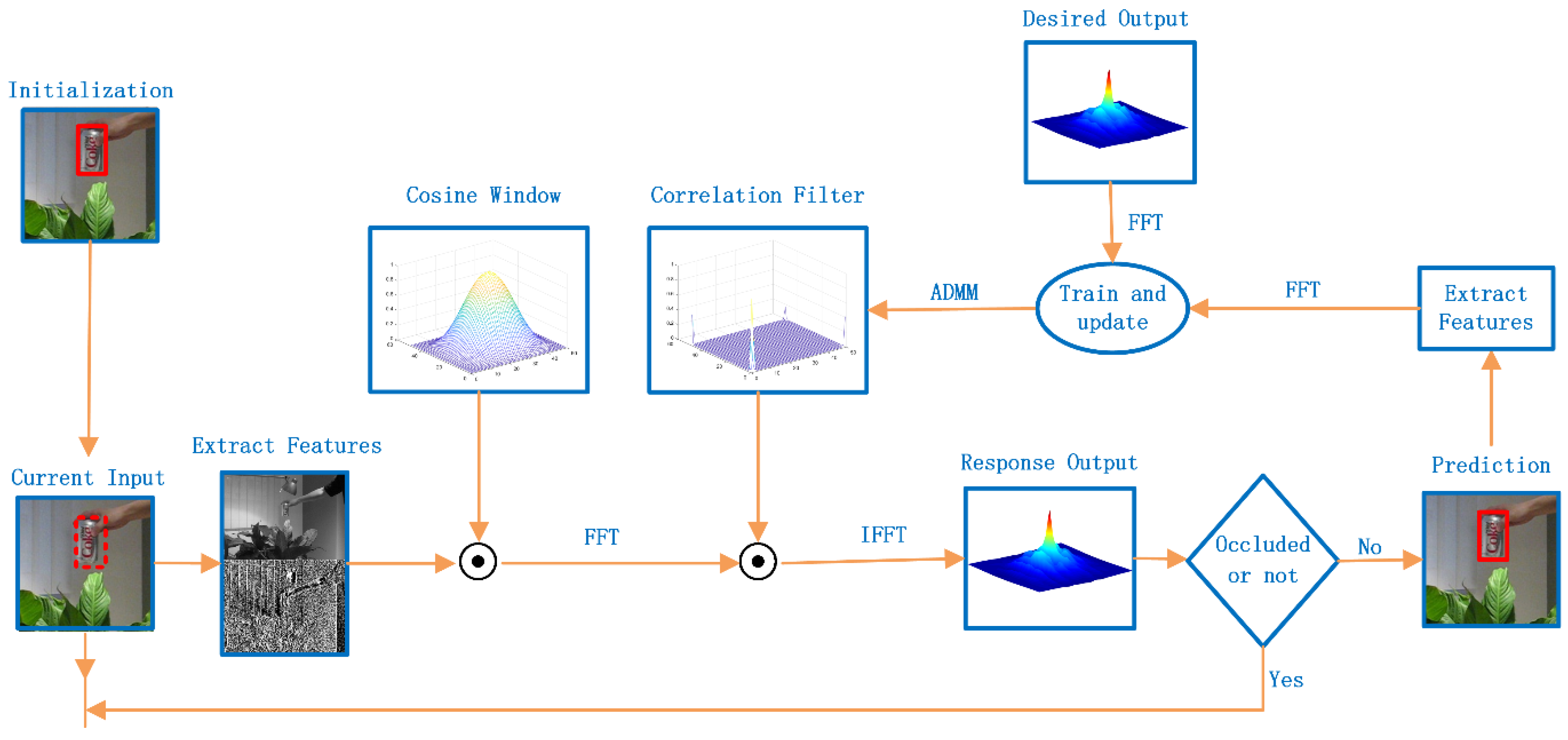
3.2. Fast Tracking Algorithm Based on Spatially Regularized Correlation Filter

The proposed fast-tracking algorithm, based on a spatially regularized correlation filter, aims to improve the speed and accuracy of the SRDCF algorithm [13]. First, this algorithm replaces the filter solver method in the SRDCF tracker from the Gauss–Seidel solver to the ADMM [14] solver, improving the computational speed and tracking efficiency. The ADMM solver uses Lagrange expressions to change the optimal solution of the large problem into two sub-problems, solved separately, and the improved algorithm sets the number of iterations of the solver to two, which can quickly obtain the approximate filter solution. Second, in the model update phase, our algorithm adds the average peak correlation energy (APCE) criterion [15] to the model update strategy, in addition to the maximum response value of the reference response map F m a x . When both the criteria F m a x and APCE of the current frame are greater than their respective historical averages by a certain ratio, the obtained tracking results are considered as high confidence, indicating that the tracking target is not occluded or lost, and the model is then updated according to the set learning rate. The tracking flow chart of the FSRCF tracker in this article is shown in Figure 1, and the structure is shown in Figure 2. The video sequence is first initialized and the first frame of the video sequence is read in order to extract the target feature information. The correlation filter model is solved using the target feature information, and the target position and scale size are calculated using the target feature information and the correlation filter model. The calculated APCE value and maximum response value are lower than the set threshold to determine whether the correlation filter should be updated or not. If the APCE value or maximum response value are lower than the set threshold, it means that the tracking is not accurate, and the correlation filter is not updated to avoid model drift. Only when the APCE value and the maximum response value are higher than the set threshold is the relevant filter updated and the tracking target is tracked in a cyclic step.

3.2.1. Improvement of the Optimization Method for Solving the Filter

The algorithm in this paper replaces the Gauss–Seidel solver with the alternating direction method of multipliers solver in the computational process of solving the filter. The specific steps of solving filter f iteratively with the ADMM solver are as follows. Filter f is one of the variables of the ADMM solver iteration, and the auxiliary variable g is introduced in the solving process, and the constraint is set as f = g.
arg min f 1 2 d = 1 D x t d f d y 2 + 1 2 d = 1 D w f d 2 s . t .   g ^ = f ^ = T F f
∧ denotes the Fourier transform, T is the size of the input picture x, and T F f is the 2D expression for the discrete Fourier transform.
The Lagrangian expression is introduced as:
( f , g ^ , ς ^ ) = 1 2 d = 1 D x ^ t d g ^ d y ^ 2 + 1 2 d = 1 D w f ^ d 2 + ς ^ T d = 1 D ( g ^ d T F f ^ d ) + μ 2 d = 1 D g ^ d T F f ^ d 2
ς is the Lagrangian vector, μ denotes the penalty factor, and the ADMM algorithm is used to solve the following subproblem iteratively. The iterative steps are as follows:
g k + 1 = 1 2 d = 1 D x ^ t d g ^ d y ^ 2 + ς ^ T d = 1 D ( g ^ d T F f ^ d ) + μ 2 d = 1 D g ^ d T F f ^ d 2 f k + 1 = 1 2 d = 1 D w f ^ d 2 + ς ^ T d = 1 D ( g ^ d T F f ^ d ) + μ 2 d = 1 D g ^ d T F f ^ d 2 ς k + 1 = ς k + μ ( g k + 1 f k + 1 )
Subproblem g:
g ^ = 1 2 d = 1 D x ^ t d g ^ d y ^ 2 + ς ^ T d = 1 D ( g ^ d T F f ^ d ) + μ 2 d = 1 D g ^ d T F f ^ d 2 = ( d = 1 D x ^ t d · x ^ t d T + T μ Ι ) 1 ( d = 1 D g ^ d · x ^ t d T T ς ^ T + d = 1 D T μ f ^ d )
Using the accelerated Sherman-Morrison formula, the solution is obtained as follows:
g ^ = 1 μ ( d = 1 D T g ^ d · x ^ t d ς ^ T + d = 1 D μ f ^ d ) d = 1 D x ^ t d μ b ( T g ^ d S ^ x S ^ ς + μ S ^ f )
Among them:
S ^ x = d = 1 D x ^ t d · x ^ t d T
S ^ ς = d = 1 D x ^ t d T · ς ^
S ^ f = d = 1 D x ^ t d T · f ^ d
b = S ^ x + T μ
Subproblem f:
f ^ = 1 2 d = 1 D w f ^ d 2 + ς ^ T d = 1 D ( g ^ d T F f ^ d ) + μ 2 d = 1 D g ^ d T F f ^ d 2 = ( w T · w + μ ) 1 ( ς ^ T + d = 1 D μ g ^ d )
Subproblem f:
ς ^ k + 1 = ς ^ k + μ ( g ^ k + 1 f ^ k + 1 )

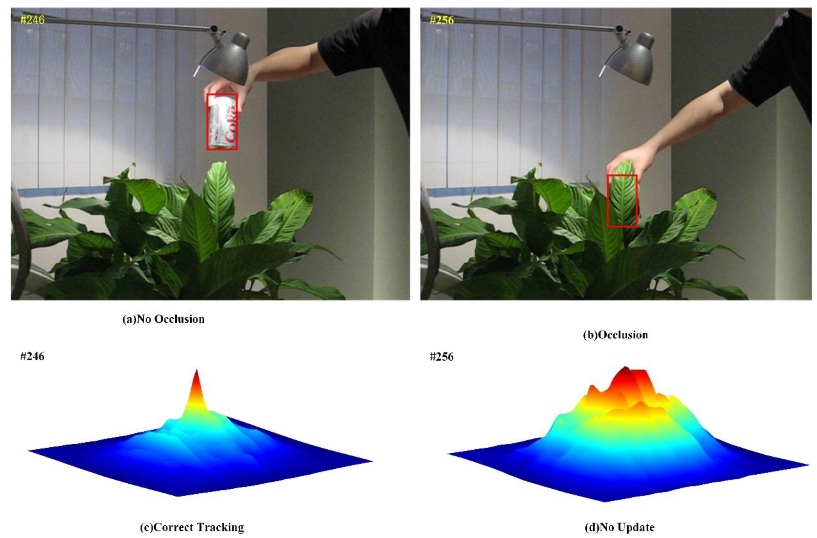
3.2.2. Occlusion Detection

Most existing trackers do not consider whether the detection is accurate or not. In fact, once a target is detected incorrectly in the current frame, for example if severe occlusion or complete loss occurs, this can lead to tracking failure in the subsequent frames. In this paper, we introduced the average peak correlation energy (APCE) criterion to determine the confidence level of the target object, and both the peak and fluctuation of the response plot show the confidence level of the tracking result. When the target is accurately tracked the response map has only one peak and all other regions are smooth. In contrast, the response map fluctuates drastically when the target is occluded. If we continue to use incorrect samples to track the target in subsequent frames, the tracking model is corrupted. Therefore, in addition to referring to the maximum response value F m a x of the response map, the average peak correlation energy (APCE) criterion is added to the model update strategy. The tracking result in the current frame is only considered as high confidence when both the criteria F m a x and APCE of the current frame are greater than their respective historical averages by a certain ratio, indicating that the tracking target is not occluded. The learning rate is then set accordingly to update the model.
The average peak correlation energy (APCE) criterion is defined as follows:
APCE = | F m a x F m i n | 2 m e a n ( w , h ( F w , h F m i n ) 2 )
where F m a x and F m i n are the maximum and minimum response of the current frame, respectively. F w , h is the element value of the w th row and h th column of the response matrix. If the tracking target is moving slowly and can be easily distinguished, the APCE value is generally high. However, if the target is moving fast and has significant deformation, the value of APCE is low even if the tracking is correct.
As shown in Figure 3c, demonstrated by sharper peaks and less noise, the target is clearly within the detection range, the response map is smooth overall, and there is only one sharp peak. This indicates that the tracking target is not obscured or lost, and the model is updated normally at this time. Otherwise, as shown in Figure 3d, if the tracking target is obscured or lost, the overall response map is disordered and has multiple peaks, which causes the target tracking model to drift and lead to target tracking failure if the model is updated.
Incorporating the APCE criteria into the model update strategy has two advantages: firstly, it solves the target model offset problem to a certain extent and thus improves the target tracking accuracy. Secondly, the model is not updated when the tracked target is occluded, thus saving computation time, and increasing the target tracking speed. Algorithm 1 shows the brief flow of the algorithm in this paper, where the APCE_Average is the total APCE values of all previous successfully tracked video frames divided by the total number of successfully tracked video frames, and the F_(max)Average is the total F_max values of all previous successfully tracked video frames divided by the total number of successfully tracked video frames.
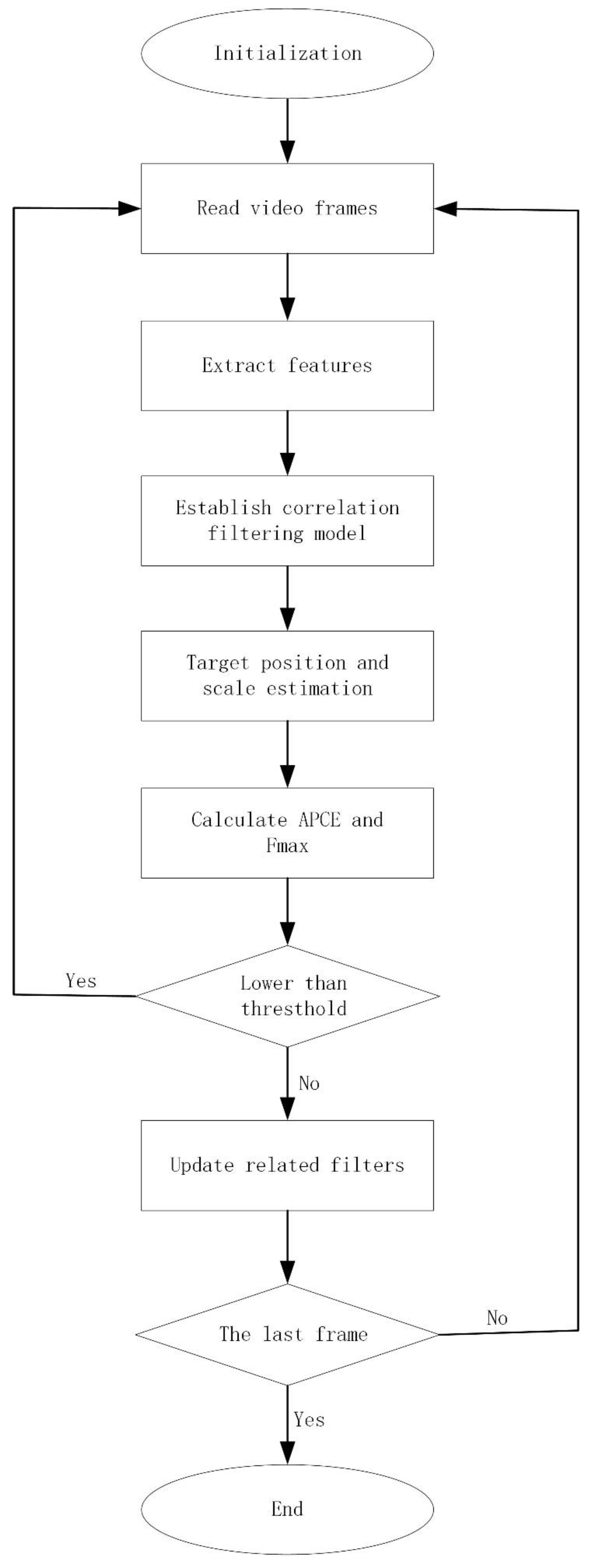
Algorithm 1: Fast Tracking Algorithm Based on Spatial Regularization Correlation Filter
Input: initial target bounding box (X, Y, W, H) and other initialization parameters
Output: target bounding box1. Enter the first frame and initialize the target filter model;
2. for the 2, 3,… until the last frame do
3. Establish 5 scales around the tracking target, and extract Gray and HOG features;
4. Use formula (2) to calculate the filter response value;
5. Determine the optimal scale of the target;
6. Use formula (14) to calculate the APCE value;
7. if APCE > 0.5 * APCE_Average and F_max > 0.6 * F_(max)Average then
8.  While ADMM iterative do
9.  use formulas (7) and (12) to solve auxiliary variables g ^   and f ^   respectively;
10.  use formula (13) to update the Lagrangian vector ς;
11.  end while
12.  Update the filter model;
13.  end if
14.  Update APCE_Average;
15. end for

4. Experiment and Analysis

To verify the performance of the algorithm, the experiments were conducted on MATLAB 2018a as the development platform, running on Windows 10 with an Intel(R) Core(TM) i5-10400 CPU @ 2.90GHz processor.

4.1. Experimental Dataset and Evaluation Criteria

4.1.1. Experimental Dataset

The OTB-2015 dataset [35] had a total of 100 video sequences, the OTB-2013 dataset [36] had a total of 51 video sequences, and the UAV123 dataset [37] had a total of 123 video sequences. Both the OTB-2015 dataset and the OTB-2013 dataset included 11 scene challenges, namely illumination change (IV), scale change (SC), occlusion (OCC), deformation (DEF), motion blur (MB), fast motion (FM), in-plane rotation (IPR), out-of-plane rotation (OPR), out of view (OV), background clutter (BC), and low resolution (LR). The UAV123 dataset contained 12 challenge scenarios, namely illumination change (IV), scale change (SC), fast motion (FM), background clutter (BC), low resolution (LR), full occlusion (FOC), partial occlusion(POC), out of view (OV), similar object (SOB), aspect ratio change (ARC), camera motion (CM), and viewpoint change(VC).

4.1.2. Experimental Evaluation Criteria

In order to compare the performance of each algorithm, we used three metrics to evaluate the algorithms in this paper. The first metric is precision. Precision is defined as the percentage of the total number of frames in the video sequence for which the difference between the center position of the tracking and the standard center position is less than a certain threshold. The percentage obtained varied by setting different thresholds, and the threshold value was set to d = 20 in this experiment.
Precision = i = 1 N f
f = { 1 ,     C L E d 0 ,     C L E > d
CLE = dis ( p 1 , p 2 )
where N denotes the number of frames in a video sequence, CLE denotes the center position error in a frame, d denotes a specific threshold, dis(-) denotes the Euclidean distance between two points, p 1 denotes the center of the tracked target, and p 2 denotes the actual target center.
The second metric is the success rate. The ratio of the area of the overlap between the tracked frame and the standard frame in the current frame to the total area covered by it is the success rate, and this is the value VOR. The tracking was considered successful if the obtained VOR value exceeded a specific threshold, which was set to d = 50 in this experiment. The success rate was calculated as the proportion of the total video that is successfully tracked and is shown as follows.
VOR = { 1 ,     k d 0 ,     k < d
Success   rate = A r e a ( B T B G ) A r e a ( B T B G )
In Equation (19), B T denotes the tracking area of the current frame, B G denotes the standard target area, ∩ denotes the overlapping area of both. and ∪ denotes the total coverage area of both.
The third metric is the speed of the tracking algorithm, which was expressed in frames per second (FPS).

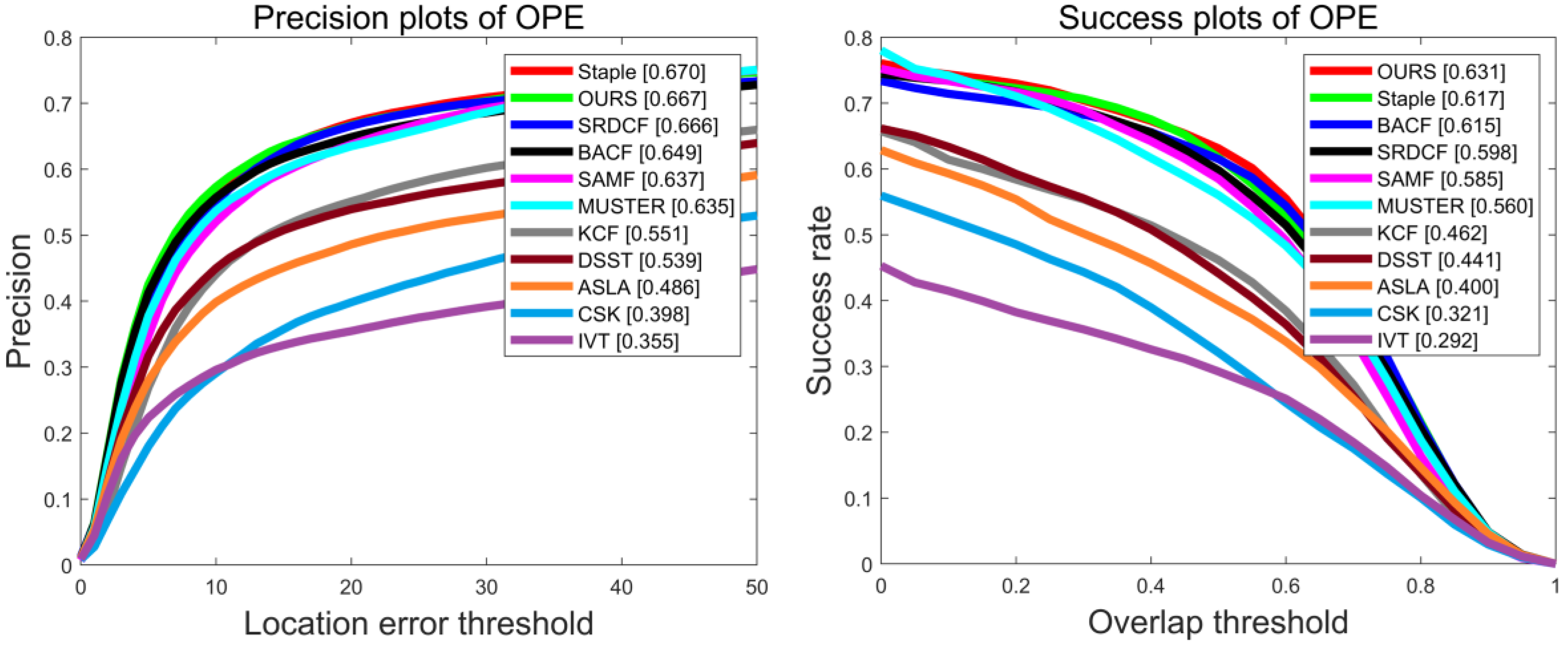
4.2. Comparative Experiments on the OTB2015 Dataset

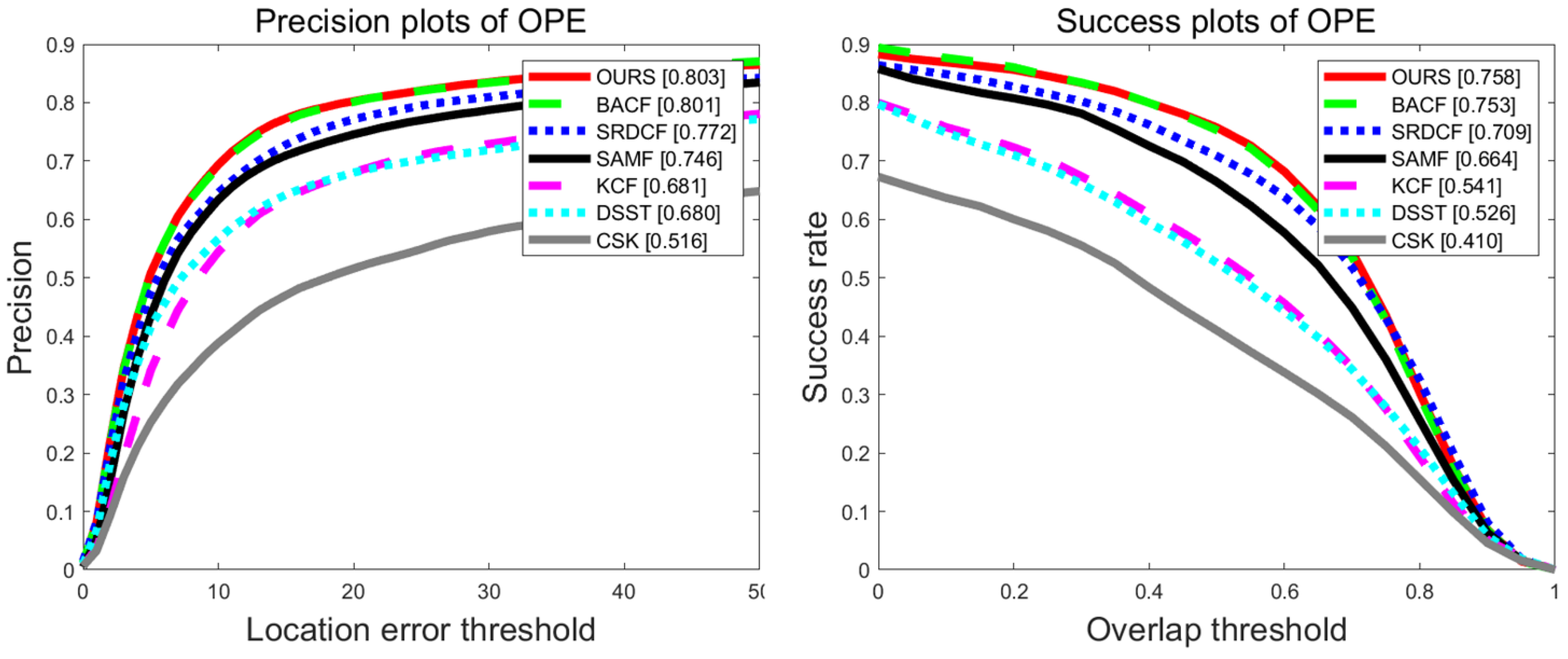
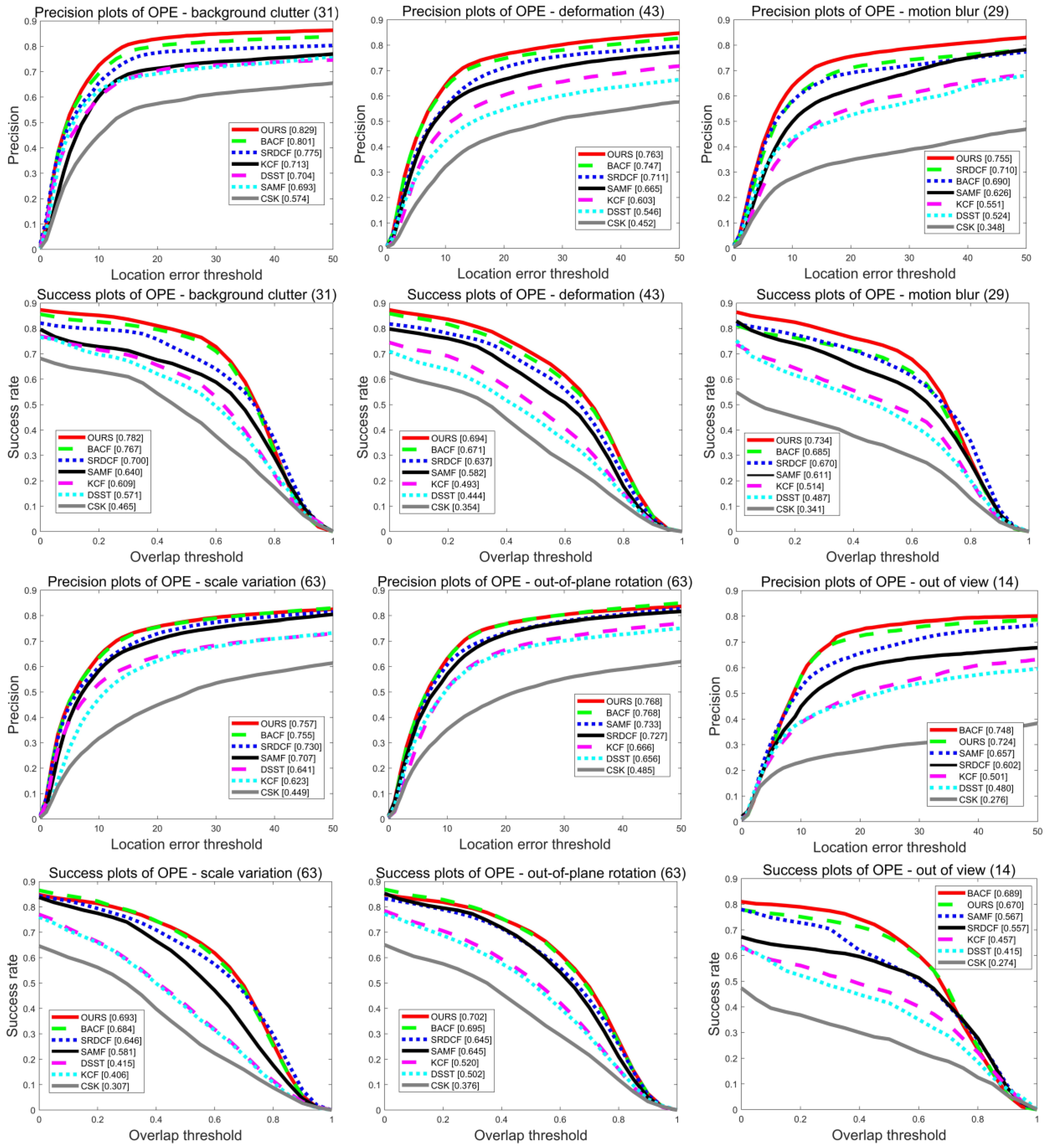
4.2.1. Quantitative Analysis

Experiments were conducted on 100 video sequences of the OTB2015 dataset, and Figure 4 shows the precision plot and success plot of seven algorithms (BACF [31], SRDCF [13], SAMF [22], KCF [12], DSST [19], CSK [11], and OURS) used in experiments on the OTB-2015 dataset. Compared with the benchmark algorithm SRDCF, the results show that our algorithm improves by 3.1% and 4.9% in precision and success rate, respectively. Compared with the BACF algorithm, the algorithm in this paper improves the accuracy by 0.2% and the success rate by 0.5%. Compared with the KCF algorithm, the algorithm in this paper improves the accuracy by 12.2% and the success rate by 21.7%. As shown in Table 1, the average performance metrics were obtained for all algorithms tested on the OTB-2015 dataset, and the bold text indicates that the current tracker’s performance ranked first in the comparison process. The algorithm in this paper improves the tracking speed from about 7 frames per second to about 29 frames per second compared to the SRDCF algorithm, enabling the tracking to achieve real-time results.
Figure 5 shows the accuracy and success rate of the algorithms regarding six attributes (background clutter (BC), deformation (DEF), motion blur (MB), scale change (SC), out-of-plane rotation (OPR), and out-of-view (OV)) of the OTB2015 dataset and shows that the algorithm in this paper performs best in the first five attributes. When the tracking target reappears in the video frame after a short time out of the field of view, only the maximum value in the response graph is used to judge whether the tracking target is inaccurate. In addition to referring to the maximum response value, this paper also integrates the APCE standard. When both criteria reach the set threshold, it was determined as a tracking target. This update strategy led to an increase of 12.2% in accuracy and 11.3% in success rate compared with the benchmark algorithm Staple in the out-of-view (OV) attribute.

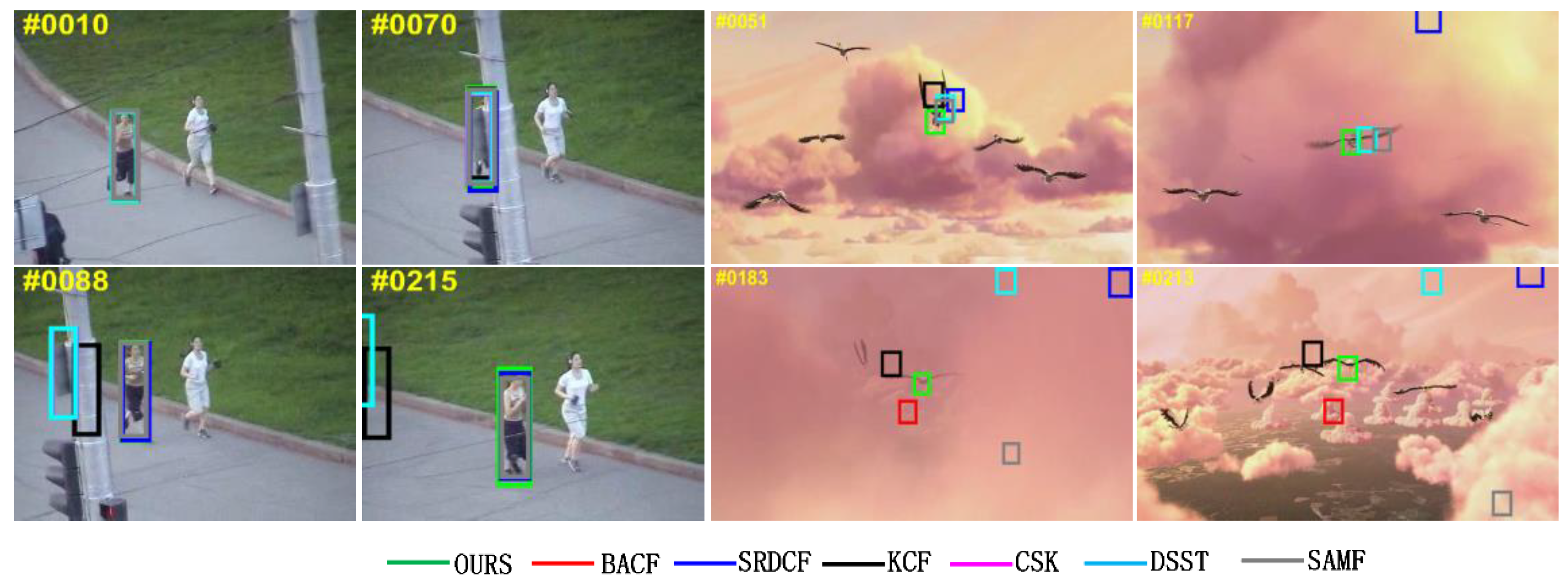
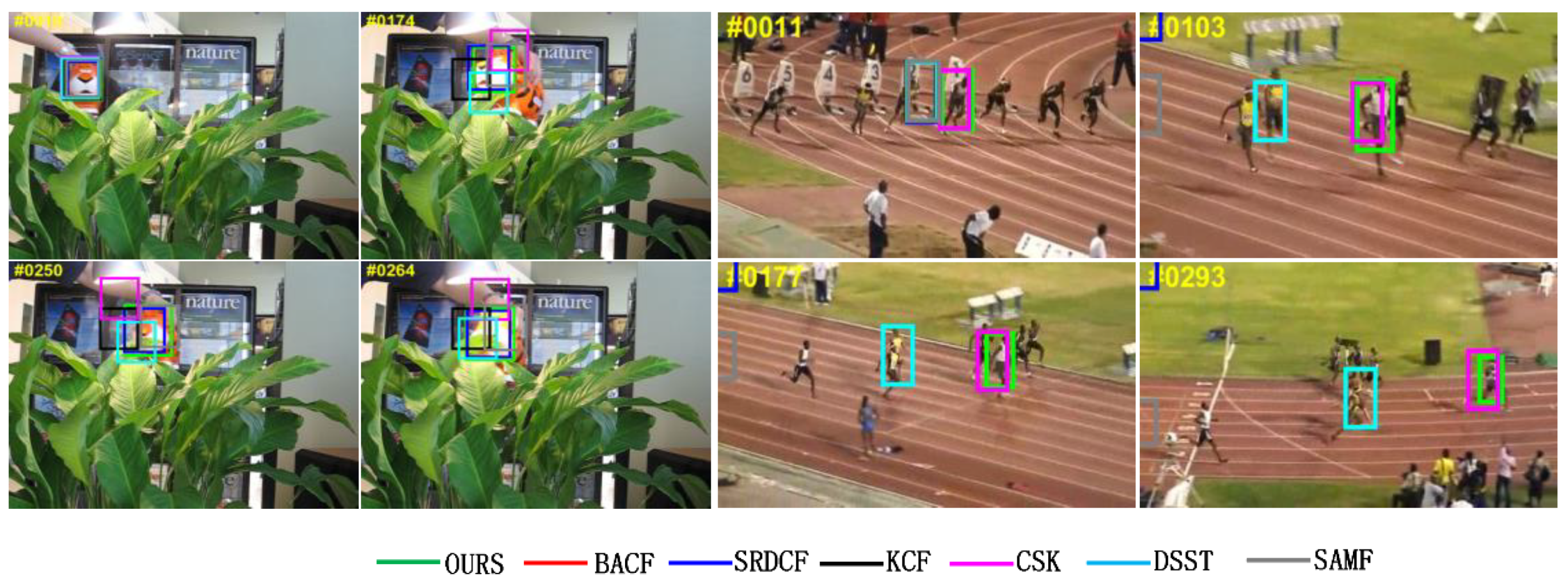
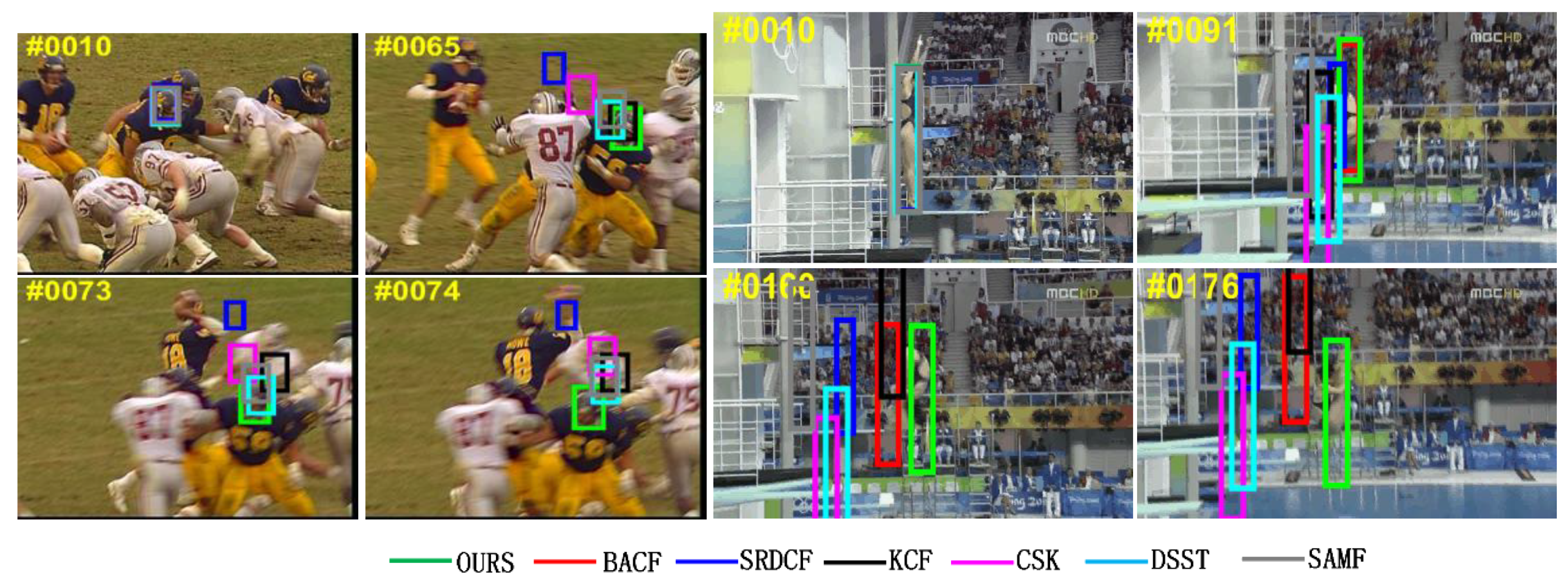
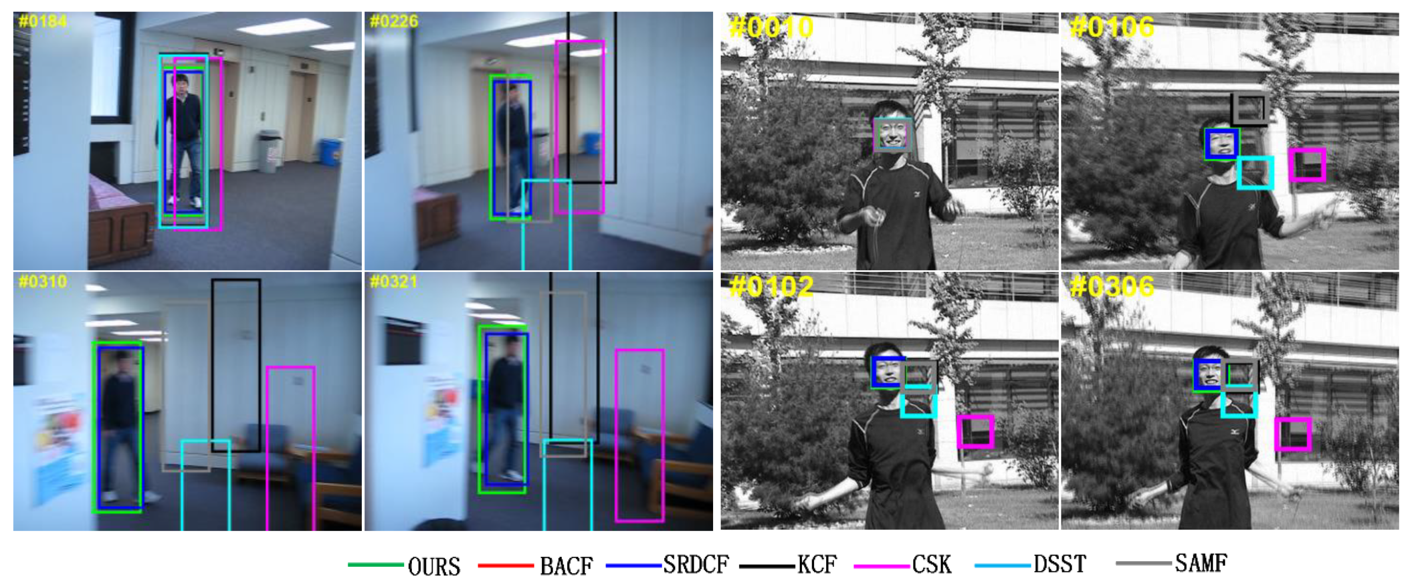
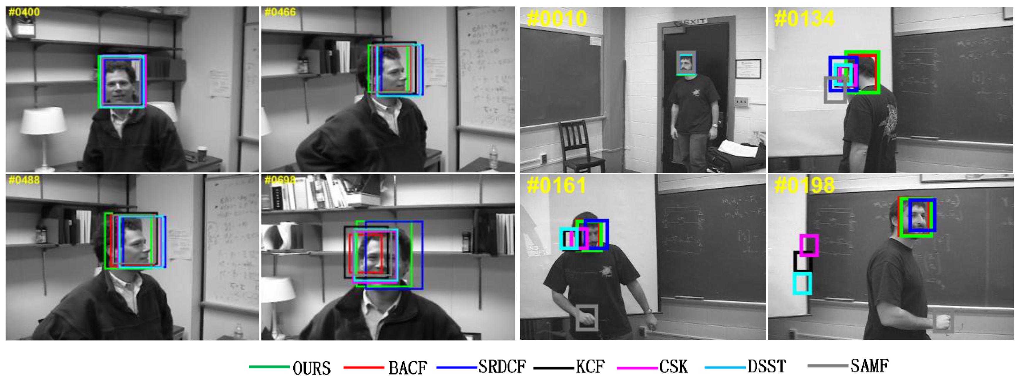
4.2.2. Qualitative Analysis

We selected 11 subsets (in the order of Jogging1, Bird1, Tiger2, Bolt2, Football1, Diving, Blurbody, Jumping, FleetFace, Freeman1, Dudek) from the OTB-2015 dataset for the comparison experiments. These 11 subsets represented multiple complex scenes of short-term target occlusion, long-term target occlusion, illumination change, scale change, background clutter, deformation, motion blur, fast motion, in-plane rotation, out-of-plane rotation, and out-of-field. Figure 6, Figure 8 and Figure 9 show the tracking results in target occlusion, background clutter, and the fast motion tracking scenes, and the algorithm in this paper maintains a strong robustness compared with the other six algorithms. The experimental results are analyzed as follows.

a: Short-Term Target Occlusion

Target occlusion contaminates the target model and leads to irreversible errors if no measures are taken to eliminate the interference caused by target occlusion. Short-time target occlusion is shown in Figure 6 Jogging1 (left). After the target encounters short-term occlusion at frame 70, the KCF, CSK, and DSST algorithms are unable to track accurately in the later frames, resulting in target tracking failure. Compared with other algorithms, the algorithm in this paper (FSRCF) has the highest tracking accuracy.

b: Long-Term Target Occlusion

As shown in Figure 6 Bird1 (right), the BACF, SRDCF, KCF, CSK, DSST, and SAMF algorithms all fail to track the target in the later frames after the target encounters long-term occlusion at frame 117. Only the FSRCF algorithm always tracked the target stably. The reason is that the algorithm in this paper uses occlusion detection, i.e., the APCE criterion is added. When occlusion occurs, the target model will not be updated, thus avoiding causing target model drift and leading to tracking failure.

c: Illumination Change

As shown in Figure 7 Tiger2 (left), the light has a normal brightness at frame 10, while the brightness increases from frame 174 to frame 264. Compared with the other six algorithms, the algorithm in this paper has the highest accuracy in tracking the target with a large change in brightness.

d: Scale Variation

The target size usually changes during tracking, so the tracker must adjust the bounding box according to the target size, otherwise it may fail due to the lack of complete target information or the acquisition of redundant background information. Figure 7 Bolt2 (right) shows the tracking results in a video sequence with scale variation, where the target scales from small to large from frame 11 to frame 103, and from large to small from frame 177 to frame 293. The SRDCF, KCF, DSST, and SAMF algorithms all failed to track this scale change. In the existing methods, two DCF-based trackers, DSST and SAMF, are designed to handle scale changes. But the DSST algorithm and SAMF algorithm cannot adapt to the scale variation in these sequences. Although the algorithm in this paper uses almost the same scale adaptation strategy as the SAMF algorithm, it still outperforms the SAMF algorithm in capturing targets with different scales.

e: Background Clutter

In Figure 8 Football (left), the tracking target is challenged by background clutter through frames 65 to 74, where the bounding box is more likely to drift onto the cluttered background. The SRDCF, KCF, CSK, DSST, and SAMF algorithms all failed to track in this situation. The successful tracking of the FSRCF algorithm is attributed to the use of the APCE criterion for occlusion detection, which enhanced the robustness of the target tracking model.

f: Deformation

In Figure 8 Diving (right), the FSRCF algorithm is able to locate and track accurately despite the deformation from frame 91 to frame 176, while the BACF, SRDCF, KCF, CSK, DSST, and SAMF algorithms all failed to track. The success of the FSRCF algorithm was due to the use of the APCE criterion for occlusion detection, which enhanced the robustness of the target tracking model.

g: Motion Blur

In Figure 9 Blurbody (left), the challenge was tracking the target through the target blur from frame 226 to frame 321. The algorithms KCF, CSK, DSST, and SAMF all failed to track, while the algorithms BACF, SRDCF, and FSRCF tracked accurately. This is related, to a large extent, to the fact that the target model of this paper’s algorithm is based on the spatial regularization of the SRDCF algorithm, which makes target tracking more accurate.

h: Fast Motion

Fast motion will blur the target and we need a larger search range to ensure that the target can be captured again. The video sequences in Figure 9 Jumping (right) are used to test the performance of these trackers in handling fast moving targets. In these sequences, only the SRDCF and FSRCF algorithms accurately tracked the target when fast motion occurred. The algorithm in this paper uses a large search window and the high confidence APCE criterion, which ensures that targets are not easily lost when moving fast.

i: In-Plane Rotation

The challenge of in-plane or out-of-plane rotation is caused by the movement or change in viewpoint of the target, and this challenge makes modeling the appearance of the target difficult. In the rotation test of the FleetFace (left) video sequence in Figure 10, none of the trackers lost their targets, but some trackers suffered from significant scale drift due to the rotation of the target in and out of the image plane. The ability of the algorithm in this paper to closely track the targets and maintain a high degree of overlap suggests that the algorithm in this paper coped well with the rotation challenge.

j: Out-of-Plane Rotation

In Figure 10 Freeman1 (right) video sequence, the SRDCF, KCF, CSK, DSST, and SAMF algorithms all failed to track in frame 134, and only the BACF algorithm and the present algorithm tracked accurately. The ability of the SRDCF algorithm to re-track the target in frames 161 to 198 may be related to the regularization component of the SRDCF algorithm, because the tracking process is used to find the maximum response value in the search range in each frame, and the regularization component can increase the background regularization strength and can re-track the target in this process.

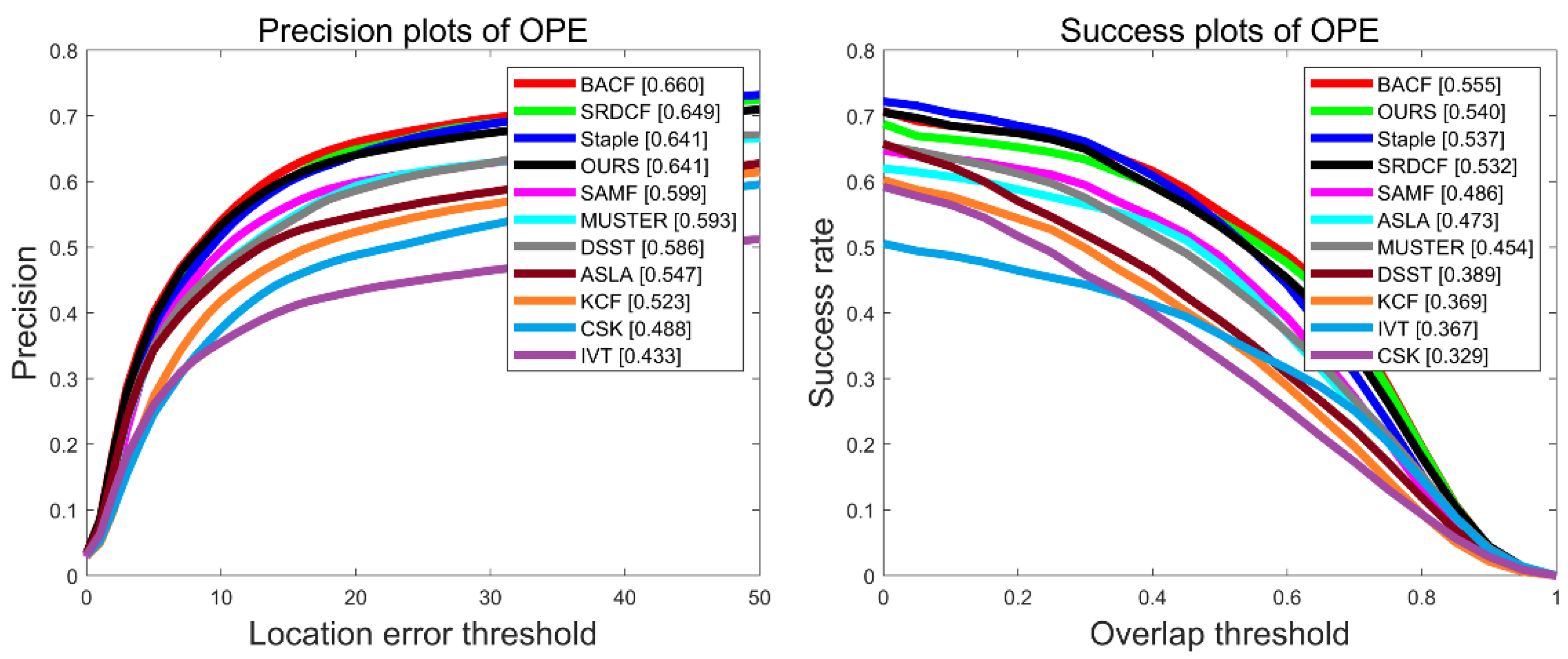
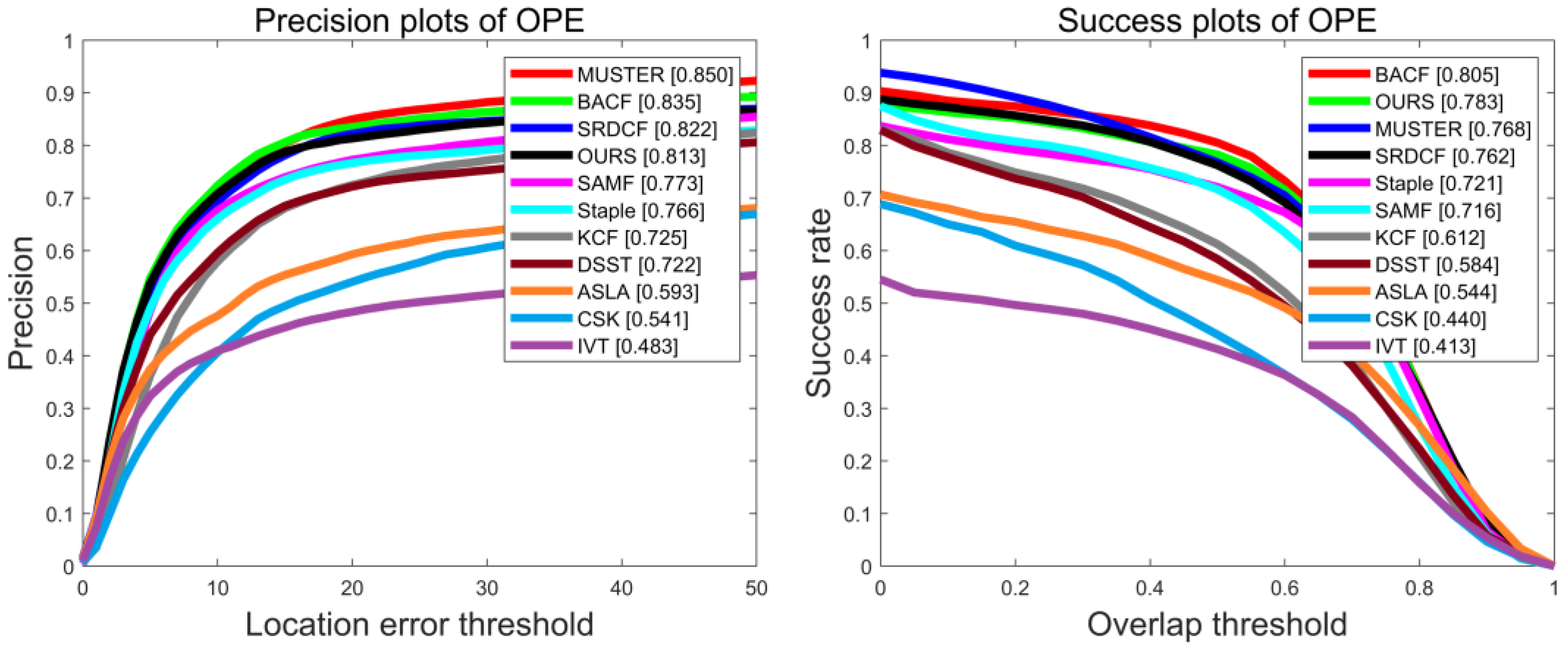
4.3. Comparative Experiments on the OTB2013 Dataset

Experiments were conducted on 51 video sequences of the OTB2013 dataset, and Figure 11 shows the precision plot and success plot of 11 algorithms (BACF [31], SRDCF [13], SAMF [22], KCF [12], DSST [19], CSK [11], Staple [25], ASLA [37], IVT [38], MUSTER [39], and OURS) tested on the OTB-2013 dataset. Compared with the benchmark SRDCF algorithm, our algorithm improves by 2.1% under the success rate criterion. Compared with the Staple algorithm, the algorithm in this paper improves the accuracy by 2% and the success rate by 0.8%. Compared with the KCF algorithm, the algorithm in this paper improves the accuracy by 8.8% and the success rate by 17.1%. As shown in Table 2, all algorithms tested on the OTB-2013 dataset obtained the average performance metrics, and the bold letters indicate that the current tracker’s performance ranked first in the comparison process. The algorithm in this paper improves the tracking speed from about 8 frames per second to about 28 frames per second compared to the SRDCF algorithm, which enables tracking to achieve real-time results.

4.4. Comparative Experiments on the UAV123 Dataset

The UAV123 dataset contained 123 video sequences taken by an unmanned aerial vehicle (UAV), including search and rescue, wildlife and crowd monitoring, and navigation, among others. The average sequence length of this dataset was 915 frames. It contained a large number of long-term video tracking sequences, which present great difficulty and challenge to the trackers. For trackers without a relocation mechanism, once model drift occurs, tracking fails. Figure 12 shows the precision plot and success plot of 11 algorithms (BACF [31], SRDCF [13], SAMF [22], KCF [12], DSST [19], CSK [11], Staple [25], ASLA [37], IVT [38], MUSTER [39], and OURS) tested on the UAV123 dataset. Compared with the benchmark algorithm SRDCF, the algorithm FSRCF improves the success rate by 0.8%. Compared with the SAMF algorithm, the algorithm in this paper improves the accuracy by 5.1% and the success rate by 5.4%. Compared with the MUSTER algorithm, the algorithm in this paper improves the accuracy by 4.8% and the success rate by 8.6%. Compared with the KCF algorithm, the algorithm in this paper improves the accuracy by 11.8% and the success rate by 17.1%. As shown in Table 3, all algorithms tested on the UAV123 dataset obtained the average performance metrics, and the bold letters indicate that the current tracker’s performance ranked first in the comparison process. The algorithm in this paper improves the tracking speed from about 12 frames per second to about 35 frames per second compared to the SRDCF algorithm, which enables tracking to achieve real-time results.

4.5. Comparative Experiments on the TC128 Dataset

Experiments were conducted on 129 color video sequences of the TC128 dataset, and Figure 13 shows the precision plot and success plot of 11 algorithms (BACF [31], SRDCF [13], SAMF [22], KCF [12], DSST [19], CSK [11], Staple [25], ASLA [37], IVT [38], MUSTER [39], and OURS) tested on the TC128 dataset. Compared with the benchmark algorithm SRDCF, our algorithm improves by 0.1% and 3.3% in precision and success rate, respectively. Compared with the BACF algorithm, the algorithm in this paper improves the accuracy by 1.8% and the success rate by 1.6%. Compared with the KCF algorithm, the algorithm in this paper improves the accuracy by 11.6% and the success rate by 16.9%. As shown in Table 4, all algorithms tested on the TC128 dataset obtained the average performance metrics, and the bold letters indicate that the current tracker’s performance ranked first in the comparison process. The algorithm in this paper improves the tracking speed from about 8 frames per second to about 35 frames per second compared to the SRDCF algorithm, which enables tracking to achieve real-time results.

5. Conclusions

In this paper, in order to alleviate the inefficiency of the SRDCF model due to the use of Gauss–Seidel solvers and the inability to track in real time, we introduced the alternating direction multiplier method solver to replace the Gauss–Seidel solver, thus improving the tracking efficiency and meeting the demand for real-time tracking. Compared with the benchmark SRDCF algorithm, the algorithm in this paper improves the tracking speed from about 7 frames per second to about 29 frames per second in the dataset OTB2015; improves the tracking speed from about 8 frames per second to about 28 frames per second in the dataset OTB2013; improves the tracking speed from about 12 frames per second to about 35 frames per second in the dataset UAV123; and improves the tracking speed from about 8 frames per second to about 35 frames per second in the dataset TC128. To avoid the common model drift problem in the field of target tracking, this paper used the maximum response value and average peak correlation energy (APCE) criteria in the model update strategy to determine the reliable part of the tracking trajectory. Incorporating the APCE criterion improved the target tracking accuracy by solving the target model drift problem to a certain extent, saved computation time, and improved the tracking speed by not updating the model when the tracked target was occluded. Experimental results show that the proposed tracker outperforms several other algorithms in tests on the OTB-2013, OTB-2015, UAV123, and TC128 datasets.

Author Contributions

Conceptualization, C.L.; methodology, C.L.; software, C.L. and A.H.; validation, C.L. and M.I.; formal analysis, C.L. and M.I.; investigation, C.L.; resources, C.L.; data curation, A.H.; writing—original draft preparation, C.L. and M.I; writing—review and editing, M.I.; visualization, C.L.; supervision, M.I. and A.H.; project administration, A.H.; funding acquisition, M.I. All authors have read and agreed to the published version of the manuscript.

Funding

This research has been funded by the National Natural Science Foundation of China (NSFC) under Grant No.62166043 and U2003207, the Natural Science Foundation of Xinjiang (No.2020D01C045), and Youth Fund for scientific research program of Autonomous Region (XJEDU2019Y007).

Institutional Review Board Statement

Ethical review and approval were waived for the above mentioned study, because all the images used in the manuscript and its experiments can be downloaded from http://cvlab.hanyang.ac.kr/tracker_benchmark/ (accessed on 30 December 2021) website for free.

Informed Consent Statement

Not applicable.

Data Availability Statement

Publicly available datasets were analyzed in this study. This data can be found here: http://cvlab.hanyang.ac.kr/tracker_benchmark/datasets.html (accessed on 30 December 2021).

Conflicts of Interest

The authors declare no conflict of interest.

References

  1. Ruan, W.; Chen, J.; Wu, Y.; Wang, J.; Liang, C.; Hu, R.; Jiang, J. Multi-correlation filters with triangle-structure constraints for object tracking. IEEE Trans. Multimed. 2018, 21, 1122–1134. [Google Scholar] [CrossRef]
  2. Greenblatt, N.A. Self-driving cars and the law. IEEE Spectr. 2016, 53, 46–51. [Google Scholar] [CrossRef]
  3. Rautaray, S.S.; Agrawal, A. Vision based hand gesture recognition for human computer interaction: A survey. Artif. Intell. Rev. 2015, 43, 1–54. [Google Scholar] [CrossRef]
  4. Shin, B.-S.; Mou, X.; Mou, W.; Wang, H. Vision-based navigation of an unmanned surface vehicle with object detection and tracking abilities. Mach. Vis. Appl. 2018, 29, 95–112. [Google Scholar] [CrossRef]
  5. Mueller, M.; Smith, N.; Ghanem, B. A Benchmark and Simulator for Uav Tracking. In European Conference on Computer Vision; Springer: Berlin/Heidelberg, Germany, 2016; pp. 445–461. [Google Scholar]
  6. Yuan, D.; Kang, W.; He, Z. Robust visual tracking with correlation filters and metric learning. Knowl.-Based Syst. 2020, 195, 105697. [Google Scholar] [CrossRef]
  7. Yuan, D.; Lu, X.; Li, D.; Liang, Y.; Zhang, X. Particle filter re-detection for visual tracking via correlation filters. Multimed. Tools Appl. 2019, 78, 14277–14301. [Google Scholar] [CrossRef] [Green Version]
  8. Liu, T.; Wang, G.; Yang, Q. Real-Time Part-Based Visual Tracking via Adaptive Correlation Filters. In Proceedings of the IEEE Conference on Computer Vision and Pattern Recognition, Boston, MA, USA, 7–12 June 2015; pp. 4902–4912. [Google Scholar]
  9. Yuan, D.; Chang, X.; Huang, P.-Y.; Liu, Q.; He, Z. Self-Supervised Deep Correlation Tracking. IEEE Trans. Image Process. 2020, 30, 976–985. [Google Scholar] [CrossRef] [PubMed]
  10. Bolme, D.S.; Beveridge, J.R.; Draper, B.A.; Lui, Y.M. Visual Object Tracking Using Adaptive Correlation Filters. In Proceedings of the 2010 IEEE Computer Society Conference on Computer Vision and Pattern Recognition, San Francisco, CA, USA, 13–18 June 2010; pp. 2544–2550. [Google Scholar]
  11. Henriques, J.F.; Caseiro, R.; Martins, P.; Batista, J. Exploiting the Circulant Structure of Tracking-by-Detection with Kernels. In European Conference on Computer Vision; Springer: Berlin/Heidelberg, Germany, 2012; pp. 702–715. [Google Scholar]
  12. Henriques, J.F.; Caseiro, R.; Martins, P.; Batista, J. High-speed tracking with kernelized correlation filters. IEEE Trans. Pattern Anal. Mach. Intell. 2014, 37, 583–596. [Google Scholar] [CrossRef] [PubMed] [Green Version]
  13. Danelljan, M.; Hager, G.; Shahbaz Khan, F.; Felsberg, M. Learning Spatially Regularized Correlation Filters for Visual Tracking. In Proceedings of the IEEE International Conference on Computer Vision, Washington, DC, USA, 7–13 December 2015; pp. 4310–4318. [Google Scholar]
  14. Boyd, S.; Parikh, N.; Chu, E.; Peleato, B.; Eckstein, J. Distributed optimization and statistical learning via the alternating direction method of multipliers. Found. Trends® Mach. Learn. 2011, 3, 1–122. [Google Scholar]
  15. Wang, M.; Liu, Y.; Huang, Z. Large Margin Object Tracking with Circulant Feature Maps. In Proceedings of the IEEE Conference on Computer Vision and Pattern Recognition, Honolulu, HI, USA, 21–26 July 2017; pp. 4021–4029. [Google Scholar]
  16. Press, W.H.; Teukolsky, S.A.; Vetterling, W.T.; Flannery, B.P. Numerical Recipes in C; Cambridge University Press: Cambridge, UK, 1988. [Google Scholar]
  17. Danelljan, M.; Shahbaz Khan, F.; Felsberg, M.; Van de Weijer, J. Adaptive Color Attributes for Real-Time Visual Tracking. In Proceedings of the IEEE Conference on Computer Vision and Pattern Recognition, Columbus, OH, USA, 23–28 June 2014; pp. 1090–1097. [Google Scholar]
  18. Possegger, H.; Mauthner, T.; Bischof, H. In Defense of Color-Based Model-Free Tracking. In Proceedings of the IEEE Conference on Computer Vision and Pattern Recognition, Boston, MA, USA, 7–12 June 2015; pp. 2113–2120. [Google Scholar]
  19. Danelljan, M.; Häger, G.; Khan, F.; Felsberg, M. Accurate Scale Estimation for Robust Visual Tracking. In Proceedings of the British Machine Vision Conference, Nottingham, UK, 1–5 September 2014. [Google Scholar]
  20. Voigtlaender, P.; Luiten, J.; Torr, P.H.; Leibe, B. Siam r-cnn: Visual tracking by re-detection. In Proceedings of the IEEE/CVF Conference on Computer Vision and Pattern Recognition, Seattle, WA, USA, 13–19 June 2020; pp. 6578–6588. [Google Scholar]
  21. Danelljan, M.; Häger, G.; Khan, F.S.; Felsberg, M. Discriminative scale space tracking. IEEE Trans. Pattern Anal. Mach. Intell. 2016, 39, 1561–1575. [Google Scholar] [CrossRef] [PubMed] [Green Version]
  22. Li, Y.; Zhu, J. A scale adaptive kernel correlation filter tracker with feature integration. In European Conference on Computer Vision; Springer: Berlin/Heidelberg, Germany, 2014; pp. 254–265. [Google Scholar]
  23. Dalal, N.; Triggs, B. Histograms of oriented gradients for human detection. In Proceedings of the 2005 IEEE Computer Society Conference on Computer Vision and Pattern Recognition (CVPR’05), San Diego, CA, USA, 20–25 June 2005; pp. 886–893. [Google Scholar]
  24. Wei, J.; Liu, F. Online Learning of Discriminative Correlation Filter Bank for Visual Tracking. Information 2018, 9, 61. [Google Scholar] [CrossRef] [Green Version]
  25. Bertinetto, L.; Valmadre, J.; Golodetz, S.; Miksik, O.; Torr, P.H. Staple: Complementary learners for real-time tracking. In Proceedings of the IEEE Conference on Computer Vision and Pattern Recognition, Las Vegas, NV, USA, 27–30 June 2016; pp. 1401–1409. [Google Scholar]
  26. Danelljan, M.; Robinson, A.; Khan, F.S.; Felsberg, M. Beyond correlation filters: Learning continuous convolution operators for visual tracking. In European Conference on Computer Vision; Springer: Berlin/Heidelberg, Germany, 2016; pp. 472–488. [Google Scholar]
  27. Danelljan, M.; Hager, G.; Shahbaz Khan, F.; Felsberg, M. Adaptive decontamination of the training set: A unified formulation for discriminative visual tracking. In Proceedings of the IEEE Conference on Computer Vision and Pattern Recognition, Las Vegas, NV, USA, 27–30 June 2016; pp. 1430–1438. [Google Scholar]
  28. Danelljan, M.; Bhat, G.; Shahbaz Khan, F.; Felsberg, M. Eco: Efficient convolution operators for tracking. In Proceedings of the IEEE Conference on Computer Vision and Pattern Recognition, Honolulu, HI, USA, 21–26 July 2017; pp. 6638–6646. [Google Scholar]
  29. Bhat, G.; Johnander, J.; Danelljan, M.; Khan, F.S.; Felsberg, M. Unveiling the power of deep tracking. In Proceedings of the European Conference on Computer Vision (ECCV), Munich, Germany, 8–14 September 2018; pp. 483–498. [Google Scholar]
  30. Kiani Galoogahi, H.; Sim, T.; Lucey, S. Correlation filters with limited boundaries. In Proceedings of the IEEE Conference on Computer Vision and Pattern Recognition, Boston, MA, USA, 7–12 June 2015; pp. 4630–4638. [Google Scholar]
  31. Kiani Galoogahi, H.; Fagg, A.; Lucey, S. Learning background-aware correlation filters for visual tracking. In Proceedings of the IEEE International Conference on Computer Vision, Venice, Italy, 22–29 October 2017; pp. 1135–1143. [Google Scholar]
  32. Lukezic, A.; Vojir, T.; Cehovin Zajc, L.; Matas, J.; Kristan, M. Discriminative correlation filter with channel and spatial reliability. In Proceedings of the IEEE Conference on Computer Vision and Pattern Recognition, Honolulu, HI, USA, 21–26 July 2017; pp. 6309–6318. [Google Scholar]
  33. Li, F.; Tian, C.; Zuo, W.; Zhang, L.; Yang, M.-H. Learning spatial-temporal regularized correlation filters for visual tracking. In Proceedings of the IEEE Conference on Computer Vision and Pattern Recognition, Salt Lake City, UT, USA, 18–23 June 2018; pp. 4904–4913. [Google Scholar]
  34. Dai, K.; Wang, D.; Lu, H.; Sun, C.; Li, J. Visual tracking via adaptive spatially-regularized correlation filters. In Proceedings of the IEEE/CVF Conference on Computer Vision and Pattern Recognition, Long Beach, CA, USA, 15–20 June 2019; pp. 4670–4679. [Google Scholar]
  35. Wu, Y.; Lim, J.; Yang, M.H. Object Tracking Benchmark. IEEE Trans. Pattern Anal. Mach. Intell. 2015, 37, 1834–1848. [Google Scholar] [CrossRef] [PubMed] [Green Version]
  36. Wu, Y.; Lim, J.; Yang, M.-H. Online object tracking: A benchmark. In Proceedings of the IEEE Conference on Computer Vision and Pattern Recognition, Portland, OR, USA, 23–28 June 2013; pp. 2411–2418. [Google Scholar]
  37. Jia, X.; Lu, H.; Yang, M.-H. Visual tracking via adaptive structural local sparse appearance model. In Proceedings of the 2012 IEEE Conference on Computer Vision and Pattern Recognition, Providence, RI, USA, 16–21 June 2012; pp. 1822–1829. [Google Scholar]
  38. Ross, D.A.; Lim, J.; Lin, R.-S.; Yang, M.-H. Incremental learning for robust visual tracking. Int. J. Comput. Vis. 2008, 77, 125–141. [Google Scholar] [CrossRef]
  39. Hong, Z.; Chen, Z.; Wang, C.; Mei, X.; Prokhorov, D.; Tao, D. Multi-store tracker (muster): A cognitive psychology inspired approach to object tracking. In Proceedings of the IEEE Conference on Computer Vision and Pattern Recognition, Boston, MA, USA, 7–12 June 2015; pp. 749–758. [Google Scholar]
Figure 1. The tracking flow diagram of the FSRCF tracker.
Information 13 00184 g001
Figure 2. Structure of the FSRCF tracker in this paper.
Information 13 00184 g002
Figure 3. Peak tracker response graph.
Information 13 00184 g003
Figure 4. Accuracy and success rate plots of different algorithms tested on the OTB-2015 dataset.
Information 13 00184 g004
Figure 5. Accuracy and success rate plots of 7 tracking algorithms tested on the BC, DEF, MB, SC, OPR, and OV attributes of the OTB2015 dataset.
Information 13 00184 g005
Figure 6. The tracking results of seven trackers on Jogging1 (left) and Bird1 (right).
Information 13 00184 g006
Figure 7. Tracking results of seven trackers on Tiger2 (left) and Bolt2 (right).
Information 13 00184 g007
Figure 8. Tracking results of seven trackers on Football1 (left) and Diving (right).
Information 13 00184 g008
Figure 9. Tracking results of seven trackers on Blurbody (left) and Jumping (right).
Information 13 00184 g009
Figure 10. Tracking results of seven trackers on FleetFace (left) and Freeman1 (right).
Information 13 00184 g010
Figure 11. Accuracy and success rate plots of different algorithms tested on the OTB-2013 dataset.
Information 13 00184 g011
Figure 12. Accuracy and success rate plots of different algorithms tested on the UAV123 dataset.
Information 13 00184 g012
Figure 13. Accuracy and success rate plots of different algorithms tested on the TC128 dataset.
Information 13 00184 g013
Table 1. Average performance of algorithms tested on the OTB-2015 dataset.
TrackerPrecision (Threshold)Success Rate (AUC)Speed (FPS)
OURS80.3%75.8%29.86
BACF80.1%75.3%34.49
SRDCF77.2%70.9%7.71
SAMF74.6%66.4%28.12
KCF68.1%54.1%306.51
DSST68.0%52.6%42.93
CSK51.6%41.0%589.15
Table 2. Average performance of algorithms tested on the OTB-2013 dataset.
TrackerPrecision (Threshold)Success Rate (AUC)Speed (FPS)
OURS81.3%78.3%28.75
SRDCF82.2%76.2%8.10
Staple79.3%75.4%44.90
SAMF77.3%71.6%33.49
KCF72.5%61.2%333.15
DSST72.2%58.4%41.48
CSK54.1%44.0%627.53
BACF83.5%80.5%36.07
MUSTER85.0%76.8%5.61
ASLA59.3%54.4%2.22
IVT48.3%41.3%43.19
Table 3. Average performance of algorithms tested on the UAV123 dataset.
TrackerPrecision (Threshold)Success Rate (AUC)Speed (FPS)
OURS64.1%54.0%35.78
BACF66.3%55.5%39.44
SRDCF64.9%53.2%12.62
Staple64.1%53.7%81.16
SAMF59.9%48.6%11.53
KCF52.3%36.9%560.31
DSST58.6%38.9%84.04
CSK48.8%32.9%1076.03
MUSTER59.3%45.4%1.88
ASLA54.7%47.3%2.76
IVT43.3%36.7%42.81
Table 4. Average performance of algorithms tested on the TC128 dataset.
TrackerPrecision (Threshold)Success Rate (AUC)Speed (FPS)
OURS66.7%63.1%35.11
BACF64.9%61.5%39.73
SRDCF66.6%59.8%8.57
Staple67.0%61.7%80.07
SAMF63.7%58.5%20.95
KCF55.1%46.2%454.76
DSST53.9%44.1%67.38
CSK39.8%32.1%847.83
MUSTER63.5%56.0%5.62
ASLA48.6%40.0%2.28
IVT35.5%29.2%37.69
Publisher’s Note: MDPI stays neutral with regard to jurisdictional claims in published maps and institutional affiliations.

