A LiDAR–Camera Fusion 3D Object Detection Algorithm

Abstract

3D object detection with LiDAR and camera fusion has always been a challenge for autonomous driving. This work proposes a deep neural network (namely FuDNN) for LiDAR–camera fusion 3D object detection. Firstly, a 2D backbone is designed to extract features from camera images. Secondly, an attention-based fusion sub-network is designed to fuse the features extracted by the 2D backbone and the features extracted from 3D LiDAR point clouds by PointNet++. Besides, the FuDNN, which uses the RPN and the refinement work of PointRCNN to obtain 3D box predictions, was tested on the public KITTI dataset. Experiments on the KITTI validation set show that the proposed FuDNN achieves AP values of 92.48, 82.90, and 80.51 at easy, moderate, and hard difficulty levels for car detection. The proposed FuDNN improves the performance of LiDAR–camera fusion 3D object detection in the car category of the public KITTI dataset.

1. Introduction

Object detection is one of the issues that has received much attention in autonomous driving. In the process of autonomous driving, cars need to detect and track objects in real-time, such as cars, bicycles, pedestrians, etc. [1]. According to the types of perception sensors, object detection can be divided into camera-based object detection, LiDAR-based 3D object detection, and LiDAR–camera fusion object detection [2].

Over recent years, camera-based 2D object detection had achieved unprecedented progress. Starting from the RCNN (Region with CNN Feature) [3], camera-based 2D object detection algorithms began to develop rapidly. A series of studies [4,5] started to use two-stage approaches, using a Region Proposal Network (RPN) to propose candidate proposals and then refining the candidate proposals for classification. Redmon et al. [6] originally proposed the one-stage object detection architecture, which provided fast and simple architecture, but the effect was not as good as the two-stage approaches. Lin et al. [7] employed a focal loss function that enables the one-stage approach to outperform the two-stage approaches in both accuracy and efficiency. Although camera-based 2D object detection algorithms had achieved excellent results, they were easily affected by factors such as lighting and weather in autonomous driving scenarios [8]. CaDDN [9] generated depth distributions for each pixel of the image and combined them with image features for camera-based 3D object detection. GUPNet [10] alleviated the error amplification problem of inference by computing deep uncertainty in monocular 3D object detection. As the depth obtained from the image was not as accurate as LiDAR, the detection performance improvement was limited.

In recent years, with the continuous improvement of LiDAR hardware, LiDAR-based 3D object detection research has increased. LiDAR-based 3D object detection mainly includes three categories: Voxel-based methods, point-based methods, and graph-based methods [11], as shown in Table 1. The voxel-based methods first divided the point clouds into voxels and then input the voxelized point clouds into the backbone network for feature extraction. For instance, VoxelNet [12] extracted features from equidistant 3D voxelized point clouds and fed them to RPN to predict 3D bounding boxes. However, VoxelNet was very slow due to the 3D convolutions. SECOND [13] improved the efficiency of VoxelNet with a sparse convolutional network (SparsConv) and improved the detection performance through data augmentation. Shi et al. [14] combined the point method with SECOND and proposed PV-RCNN, which achieved high detection results. After PV-RCNN, the voxel-based methods could not be improved on a large scale. The point-based methods directly extracted features from point clouds. Since PointNet [15] and PointNet++ [16] could effectively extract point cloud features, they were used as a backbone by many methods. PointRCNN [17] used PointNet++ as the backbone to extract the features of point clouds and generate candidate boxes. The candidate boxes were then refined to generate the final detection results. STD [18], which had a high recall and low computational time, adopted a spherical anchor mechanism to generate proposals and implemented a parallel intersection-over-union (IoU) branch to improve positioning accuracy and detection performance. The graph-based methods used a graph neural network (GNN) to extract features of point clouds. For example, Point-GNN [19] efficiently encoded point clouds in a fixed-radius nearest-neighbor graph and used a GNN to obtain the 3D box predictions. Since the LiDAR point cloud of distant objects is very sparse, it encounters difficulties in detecting distant or small objects [20]. Moreover, the LiDAR point cloud provides little color and texture information, which limits further performance improvements [21].

Recently, some studies have explored LiDAR–camera fusion object detection methods, as shown in Table 1. Some multi-view methods transformed point clouds into a bird’s-eye view (BEV), front view (FV), or range view (RV), and then fused the features of these views with image features [22,23]. For instance, MV3D [24] generated 3D object proposals from BEVs, which were projected to BEVs, FVs, and image views. The features of different views were then fused to predict 3D object-bounding boxes. AVOD [25] extended MV3D to extract equal-sized features from BEVs and image views and then fused these features using an average pooling operation. The disadvantages of multi-view methods are computationally intensive and time-consuming. Some frustum-based methods utilized existing 2D detectors to generate frustum proposals in the image and then learned the corresponding frustum point cloud features for 3D box predictions. For instance, Frustum PointNet [26] generated 2D object region proposals in images via a CNN, and then extruded each 2D region to a 3D frustum. Finally, PointNet was used to predict a 3D bounding box of each object from the points in the frustum. The performances of frustum-based methods are easily limited by 2D image detectors. Later methods tended to design independent backbone networks to extract features from RGB images and raw LiDAR point clouds, and then the two kinds of features were fused for 3D box predictions. For instance, 3D-CVF [27] used an image backbone to extract image features and converted them to BEV domain features. Next, a gated feature fusion network was utilized to combine image features with point cloud features. At last, a fusion network based on the 3D region of interest (ROI) was used to refine proposals and predict the output. EPNet [28] fused image features with point cloud features five times, which improved the prediction performance. PI-RCNN [29] proposed a multi-task LiDAR–camera fusion object detection method that combined image segmentation and 3D detection. These methods using two independent feature extractors have made progress, but the performance needs to be further improved [30].

Table 1. Classification of different methods using LiDAR.

Modality	Method Category	Method
LiDAR-based	Voxel-based methods	VoxelNet [12], SECOND [13], PV-RCNN [14],
	Point-based methods	PointNet [15], PointNet++ [16], PointRCNN [17], STD [18]
	Graph-based methods	Point-GNN [19]
LiDAR–camera fusion	Multi-view methods	MV3D [24], AVOD [25]
	Frustum-based methods	Frustum PointNet [26]
	Independent backbone methods	3D-CVF [27], EPNet [28], PI-RCNN [29]

Table 1. Classification of different methods using LiDAR.

Modality	Method Category	Method
LiDAR-based	Voxel-based methods	VoxelNet [12], SECOND [13], PV-RCNN [14],
	Point-based methods	PointNet [15], PointNet++ [16], PointRCNN [17], STD [18]
	Graph-based methods	Point-GNN [19]
LiDAR–camera fusion	Multi-view methods	MV3D [24], AVOD [25]
	Frustum-based methods	Frustum PointNet [26]
	Independent backbone methods	3D-CVF [27], EPNet [28], PI-RCNN [29]

Focusing on the problem that the accuracy of LiDAR–camera fusion object detection methods is not high enough, this work proposes a new deep neural network (namely FuDNN) for LiDAR–camera fusion 3D object detection. First, a 2D backbone is proposed to learn 2D features from camera images. Second, an attention-based fusion sub-network is designed to fuse the 2D features and the 3D features extracted from 3D LiDAR point clouds. Finally, the FuDNN is verified in the experiments using the KITTI [31] 3D object detection benchmark dataset. The major contributions of this work are two-fold. First, the proposed 2D backbone has a more compact structure than the commonly used 2D backbones but has better performance. Second, the proposed attention-based fusion sub-network only needs to fuse point cloud features and image features once to achieve better results. The follow-up content is organized as follows: Section 2 introduces the architecture of FuDNN and the overall loss function. Section 3 elaborates the KITTI dataset, the FuDNN training, the performance metrics, and the analysis of the results. Section 4 provides a summary of the entire work and the follow-up research directions.

2. FuDNN for 3D Object Detection

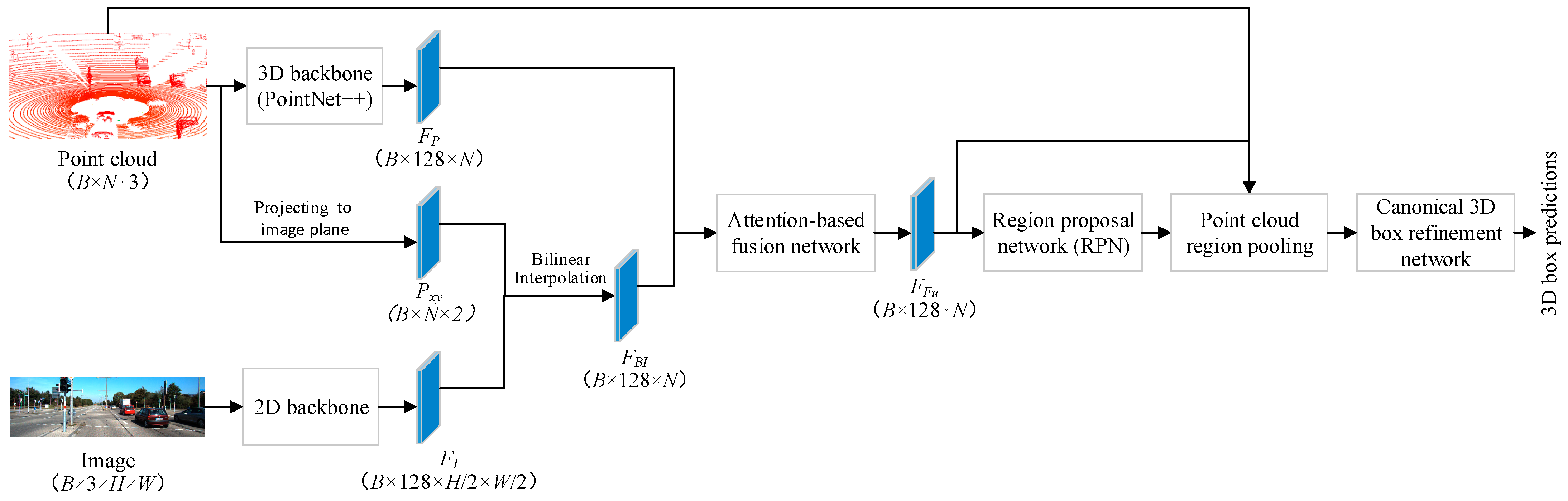
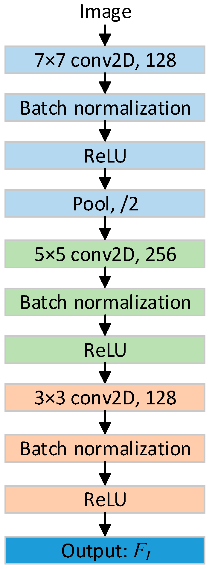
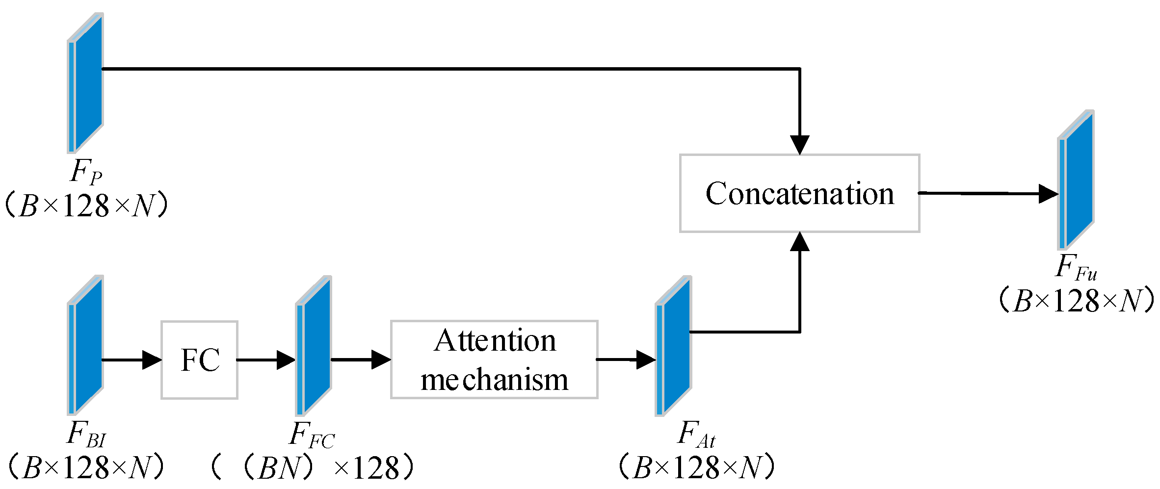
2.1. FuDNN Architecture

A deep learning network based on PointRCNN, named FuDNN, is designed to realize 3D object detection. The architecture of FuDNN is shown in Figure 1, including a 2D backbone, a 3D backbone, an attention-based fusion sub-network, an RPN, and a 3D box refinement network. The 2D backbone is designed to learn 2D features from camera images automatically, and the attention-based fusion sub-network is proposed to fuse the 2D features with the 3D features extracted by PointNet++. The RPN and 3D box refinement network of PointRCNN are used to generate 3D proposals and refine the 3D box locations, respectively.

The input of FuDNN is point clouds and RGB images. The shape of input images is a matrix of B × 3 × H × W, where B, H, and W represent the batch size of FuDNN, the height, and the width of the image, respectively. The shape of input point clouds is a matrix of B × 3 × N, where N is the number of LiDAR points.

The architecture of the 2D backbone is shown in Figure 2. The first layer (Conv1) of the 2D backbone is a 2D convolutional layer with 128 convolution kernels, each 7 × 7, using a stride of 1. The output of Conv1 is a matrix of B × 128 × H × W. The research of Ioffe and Szegedy [32] showed that the batch normalization method could speed up network convergence and reduce training difficulty, so a batch normalization layer (BN1) was used after Conv1. A rectified linear unit layer (ReLU1) is added after the BN1 layer to avoid gradient disappearance. The output shape of BN1 and ReLU1 is the same as that of Conv1. To reduce the amount of calculation, a max-pooling layer (S1) with a kernel size of 2 × 2 is adopted after ReLU1, and its output shape is B × 128 × H/2 × W/2. Next, the similar structures repeat two times: The 2D convolutional layer (Conv2) with 256 convolution kernels, each 5 × 5, is followed by the batch normalization layer (BN2). Then there is the ReLU2. At last, the 2D convolutional layer (Conv3) with 128 convolution kernels, each 3 × 3, is followed by the ReLU3. The 2D backbone outputs the image feature matrix $F_I$ of the shape B × 128 × H/2 × W/2.

Since point cloud features and image features lack correspondence, it is necessary to establish the correspondence between image features and point cloud features before projecting the point clouds to the image plane. The point clouds (x, y, z) are mapped to the image plane (u, v) via a transformation matrix M, as shown in Equations (1) and (2):

$${\left(u, v, 1\right)}^T=M·{\left(x, y, z, 1\right)}^T$$

(1)

$$M=P_{rect}·\left(\begin{array}{cc}{R}_{LiD}^{cam}& t_{LiD}^{cam}\\ 0& 1\end{array}\right)$$

(2)

where $P_{rect}$ is the projection matrix, $R_{LiD}^{cam}$ is the 3 × 3 rotation matrix, and $t_{LiD}^{cam}$is the 1 × 3 translation vector from the LiDAR to the camera, respectively. Projecting the point clouds to the image plane obtains a B × N × 2 matrix$P_{xy}$.

The point cloud feature$F_P$ and the image feature$F_I$ need to have the same dimension to be fused, so the bilinear interpolation method is used to sample$F_I$ to obtain the same dimension as$F_P$. First, $P_{xy}$is expanded from B × N × 2 to obtain a B × 1 × N × 2 matrix. Second, with the B × 1 × N × 2 matrix as the guide map, $F_I$ is sampled by bilinear interpolation to obtain the feature map of B × 128 × 1 × N, which is then removed by the dimension of 1 to obtain the final feature map $F_{BI}$ of B × 128 × N.

Figure 3 shows the structure of the attention-based fusion sub-network. Since pictures are easily affected by light and occlusion and introduce interference information, an attention mechanism is introduced to weight image features according to their importance. Before applying the attention mechanism, $F_{BI}$ is fed to the fully connected layer to obtain the vector$F_{FC}$ with the shape BN × 128. Then, the attention mechanism is applied to$F_{FC}$, as shown in Equations (3)–(5). Among them, $w$and b are parameters learned during training to obtain the hidden representation $h$from the input$F_{FC}$. The shape of $h$ is BN × 128. The multiplication result of $F_{FC}$ and $w$ is a matrix product. The vector$u_w$, which is randomly initialized and learned during training, is introduced to capture context. The similarity is used as a measure of importance and is obtained by the matrix product of $h$and$u_w$. The similarity is processed by the sigmoid function to obtain the normalized attention weight vector$a$ with the shape BN × 1. Then $a$ is transformed into B × 1 × N. The output of the attention mechanism is$F_{Att }$, which is obtained by the dot product of $a$ and$F_{FC}$. Finally, $F_{Att }$ is concatenated with $F_P$ to obtain the fused feature$F_{Fu}$.

$$h=\tanh \left(w{F}_{FC}+b\right)$$

(3)

$$a=\mathrm{sigmoid}\left(h^T{u}_w\right)$$

(4)

$$F_{Att}=a{F}_{FC}$$

(5)

The RPN of PointRCNN is utilized to generate 3D bounding box proposals. Given the images and point cloud fused features$F_{Fu}$, a segmentation head is used to estimate the foreground mask, and a box regression head is used to generate 3D proposals. The 3D proposals are generated from segmented foreground points, which avoids using a large number of pre-defined 3D boxes in 3D space. The 3D points and corresponding point features are pooled according to the location of each 3D proposal to eliminate proposals without interior points. The canonical 3D box refinement network of PointRCNN is employed to refine the box locations and finally obtain 3D box predictions.

2.2. Overall Loss Function

The overall loss function is mainly based on PointRCNN, and the consistency enforcing te loss of EPNet is introduced. The proposed FuDNN is optimized with a loss function${ℒ}_{total}$, which is the sum of the RPN loss ${ℒ}_{rpn}$and the refinement network loss${ℒ}_{refine}$. The loss function${ℒ}_{total}$ can be formulated as:

$${ℒ}_{total}={ℒ}_{rpn}+{ℒ}_{refine}$$

(6)

The RPN loss${ℒ}_{rpn}$consists of the classification loss${ℒ}_{cls}$, regression loss${ℒ}_{reg}$, and consistency enforcing loss${ℒ}_{ce}$, as shown in Equation (7). The focal loss [33] is used as ${ℒ}_{cls}$ to balance positive and negative samples for classification, as shown in Equation (8). The parameters of focal loss keep the default values of $c$ = 0.25 and $r$ = 2. The definition of ${ℒ}_{ce}$ is shown in Equation (9), where D denotes the predicted bounding box, G denotes the ground truth, and k denotes the classification confidence of D.

$${ℒ}_{rpn}={ℒ}_{cls}+{ℒ}_{reg}+\lambda {ℒ}_{ce}$$

(7)

$${ℒ}_{cls}=-c{\left(1-p_t\right)}^r\log p_t$$

(8)

$${ℒ}_{ce}=-\log \left(k\times \frac{Area\left(D{{\displaystyle \cap }}^{ }G\right)}{Area\left(D{{\displaystyle \cup }}^{ }G\right)}\right)$$

(9)

The regression loss ${ℒ}_{reg}$is used to constrain the bounding box$\left(x,y,z,h,w,l,\theta \right)$, where $\left(x,y,z\right)$is the center, $\left(h,w,l\right)$ is the size, and $\theta$ is the orientation. PointRCNN divides each foreground point-surrounding area into bins along the X and Z axes, and ${ℒ}_{reg}$ is the bin-based regression loss. The calculation process of${ℒ}_{reg}$ is as follows:

$${ℒ}_{bin}={\displaystyle \sum }_{uϵ\left\{x,z,\theta \right\}}\left(E\left({\widehat{b}}_u,b_u\right)+S\left({\widehat{r}}_u,r_u\right)\right)$$

(10)

$${ℒ}_{res}={\displaystyle \sum }_{vϵ\left\{y,h,w,l\right\}}S\left(r_v,{\widehat{r}}_v\right)$$

(11)

$${ℒ}_{reg}=\frac{1}{N_{pos}}{\displaystyle \sum }_{pϵpos}\left({ℒ}_{bin}+{ℒ}_{res}\right)$$

(12)

where E represents the cross-entropy loss, S represents the smooth L1 loss, ${\widehat{b}}_u$ and $b_u$are the predicted bin assignments and the ground-truth bin assignments, ${\widehat{r}}_u$ and $r_u$ are the residuals and the ground-truth residuals, and $N_{pos}$ is the number of foreground points. Each residual is a variable for further optimizing the position of the specified bin, and its calculation process is detailed in PointRCNN.

3. Experiments and Analysis

3.1. Dataset

The KITTI 3D object detection benchmark dataset is used as the experimental dataset. KITTI was collected by an equipment platform fixed on the top of the car, including two grayscale cameras, two color cameras, a Velodyne 64-line 3D LiDAR, four optical lenses, and one GPS/IMU system. KITTI was sampled and synchronized at 10 Hz, including 7481 training samples and 7581 testing samples. Each sample provides both the point cloud and the camera image. The labels of KITTI were divided into three subsets: Easy, moderate, and hard, according to the heights of their 2D bounding boxes, occlusion levels, and truncation levels. The easy difficulty level has a minimum 2D bounding box height of 40 Px, an occlusion level of full visibility, and a maximum truncation level of 15%. The minimum 2D bounding box height, occlusion level, and maximum truncation level of moderate difficulty level are 25 Px, partial occlusion, and 30%, respectively. The minimum 2D bounding box height for the hard difficulty level is 25 Px, the occlusion level is hard to see, and the maximum truncation level is 50%.

The image data of color camera 2 and the point cloud data of Velodyne LiDAR are used in this work. Since the test samples of KITTI are not labeled, the approach of Shi et al. [17] is adopted to further divide the training samples into 3712 samples for training and 3769 samples for validation. Only visible objects in the image are labeled, so according to the general practice of previous studies [19,24], only the LiDAR points projected into the image are used. The LiDAR points are mapped at the camera coordinates X (right) axis [−40, 40] meters, Y (down) axis [−1, 3] meters, and Z (forward) axis [0, 70.4] meters. The range of point clouds is [−π, π].

3.2. FuDNN Training

The experiments were carried out on a server with the Ubuntu 16.04.1 LTS system. The server GPU was GeForce RTX 3090 24 GB, the CPU was Intel [email protected] GHz, and the RAM size was 256 GB. The main installation packages required by the running environment of the program are shown in

Table 2. Main installation packages required by the running environment.

Package Name	Version
Python	3.7.6
CUDA	11.3
PyTorch	1.10.1
TensorboardX	2.4.1
Numpy	1.21.2
Pillow	8.4.0
Numba	0.54.1
Opencv-python	4.5.5.62
Torchvision	0.11.2

.

The FuDNN was trained in an end-to-end manner. During the data preprocessing stage, the images were scaled to a uniform size of 384 × 1280. Each point cloud was subtracted or supplemented to ensure that the number of points in each point cloud was 16,384. Several data augmentation techniques were employed on the point clouds to avoid over-fitting, which are widely used in [1,12,13], including flip (along the forwarding axis), random scaling (scale factor 0.95∼1.05 for all 3 axes), and rotation (−10∼10 degrees along the vertical axis). The data augmentation was only used for training. During network training, the network parameters were optimized by the Adam method [34]. The initial learning rate and weight decay of the network were set to 0.002 and 0.001, respectively. The model was trained for 150 epochs with a batch size of 4 and saved every 5 epochs. The threshold of IoU was set to 0.7 to distinguish between true positives and false positives.

3.3. Performance Metrics

According to the latest rules of KITTI, the 40-point Interpolated Average Precision metric was used as the performance metric, as shown in Equation (13):

$$\mathrm{AP}{|}_{R_{40}}=\frac{1}{\left|R_{40}\right|}{\displaystyle \sum }_{r\in R_{40}}{\rho }_{interp}\left(r\right)$$

(13)

where R₄₀ = {1/40,2/40,3/40, …,1} and |R₄₀| = 40. The interpolation function ${\rho }_{interp}$ is defined as:

$${\rho }_{interp}\left(r\right)=\underset{r^{\prime }:r^{\prime }\ge r}{\max }\rho \left(r^{\prime }\right)$$

(14)

where $\rho \left(r\right)$ is the precision at recall r. ${\rho }_{interp}\left(r\right)$is the value at recall $r$ on the smoothed precision–recall curve, not the actual precision values $\rho \left(r\right)$. Furthermore, ${\rho }_{interp}\left(r\right)$ is greater than or equal to$\rho \left(r\right)$.

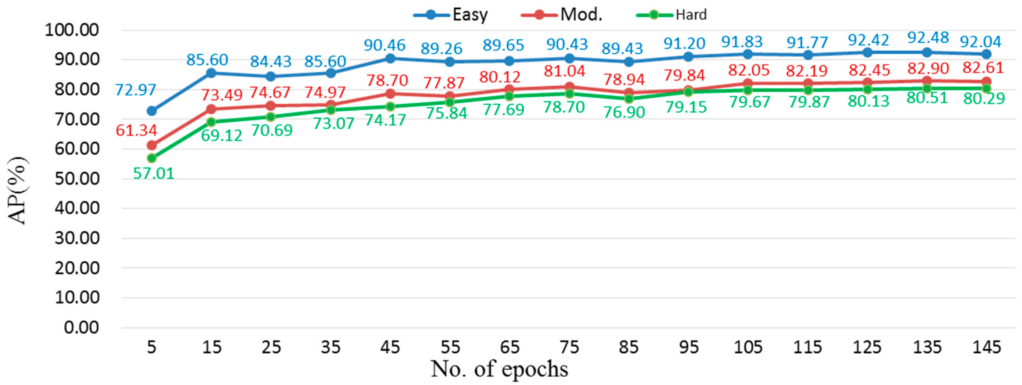
3.4. Results and Discussion

Since the car category of KITTI provided enough samples, the experiments in this work were all conducted in the car category. KITTI divided the samples of the car category into three difficulty levels, easy, moderate, and hard, so the verification experiments of this work evaluated the three levels of difficulty, respectively. Figure 4 shows the relationship between the AP of FuDNN and the number of training epochs. When the epoch number increased from 5 to 45, the AP values increased rapidly. The AP values increased flatly after epoch 45. When the epoch number was 135, the AP values reached the maximum at the three difficulty levels of easy, moderate, and hard, which were 92.48, 82.90, and 80.51, respectively. When the epoch number was greater than 135, the AP values did not exceed that of epoch 135. Therefore, the model of epoch 135 was used as the best-trained model.

Table 3. AP comparison of different 3D object detection algorithms in the car class of KITTI validation set with IoU threshold 0.7.

Method	Modality	Easy	Moderate	Hard	Speed (fps)
PointPillars [1]	LiDAR-based	87.75	78.39	75.18	62.0
SECOND [13]	LiDAR-based	90.97	79.94	77.09	26.3
PointRCNN [17]	LiDAR-based	92.54	82.16	77.88	10.0
3D-CVF [27]	LiDAR–camera fusion	89.67	79.88	78.47	13.3
EPNet [28]	LiDAR–camera fusion	92.28	82.59	80.14	10.0
PI-RCNN [29]	LiDAR–camera fusion	88.27	78.53	77.75	11.1
FuDNN (Proposed)	LiDAR–camera fusion	92.48	82.90	80.51	10.5

shows the AP comparison between the proposed FuDNN and the previous methods on the car class of KITTI validation set with the IoU threshold of 0.7. The AP values of FuDNN in the moderate and hard difficulty levels were higher than those of other methods. At the easy difficulty level, the AP value of FuDNN reached 92.48, which was 4.73 higher than the lowest PointPillars [1], but slightly lower than the best PointRCNN [17]. At the moderate difficulty level, the AP value of FuDNN showed a 4.51 improvement over the lowest PointPillars and a 0.31 improvement over the best EPNet [28]. At the hard difficulty level, the AP value of FuDNN outperformed the lowest PointPillars and the best EPNet by 5.33 and 0.37, respectively. Although the AP value of FuDNN was 0.06 lower than PointRCNN at the easy difficulty level, it was 0.74 and 2.63 higher than PointRCNN at moderate and hard difficulty levels, respectively. PointPillars achieved a speed of 62.0 fps, but its AP values were too low. SECOND was also fast, reaching 26.3 fps, but its AP values were lower than the proposed FuDNN. The speed of FuDNN was similar to PointRCNN, 3D-CVF, EPNet, and PI-RCNN. Therefore, the overall effect of FuDNN was better than that of PointRCNN. The above comparisons demonstrated the effectiveness of FuDNN. Since the car samples in the KITTI dataset all have different degrees of occlusion and truncation, the AP of object detection will be limited. Especially for the hard difficulty level, the occlusion level is hard to see, and the cutoff level is 50%, so it is very important to improve the AP value.

Table 4. Ablation experiments of different 2D backbones in the car class of KITTI validation set with IoU threshold 0.7.

Model	2D backbone	Easy	Moderate	Hard
A	Resnet50 [35]	91.75	81.22	79.620
B	Resnet101 [35]	92.24	81.87	80.03
C	VGG16 [36]	91.70	80.80	79.11
D	DensNet121 [37]	92.46	82.05	79.97
FuDNN	Proposed	92.48	82.90	80.51

shows a set of ablation experiments to compare the effects of different 2D backbones in the car class of the KITTI validation set with an IoU threshold of 0.7. Models A, B, C, and D were obtained by replacing the 2D backbone of FuDNN with Resnet50 [35], Resnet101 [35], VGG16 [36], and DensNet121 [37], respectively. The AP values of model B and model D were higher than those of model A and model C at all three difficulty levels. The reason may be that model B and model D had more network layers to extract richer feature information. The proposed 2D backbone of FuDNN not only had the simplest structure but also had the highest AP values across all three difficulty levels. This set of experiments demonstrated the effectiveness of the proposed 2D backbone.

Another set of ablation experiments was designed to analyze the effect of different fusion modes, as shown in

Table 5. Ablation experiments of different fusion methods in the car class of KITTI validation set with IoU threshold 0.7.

Model	Fusion Method	Easy	Moderate	Hard
E	Addition	91.99	82.26	80.17
F	Attention-based Addition	92.74	82.76	80.50
G	Concatenation	92.13	81.91	79.96
FuDNN	Attention-based Concatenation	92.48	82.90	80.51

. Model G removed the attention mechanism based on FuDNN, and model F changed the concatenation of FuDNN to point-wise addition. Model E removed the attention mechanism based on model F. The AP values of FuDNN across three difficulty levels were all higher than those of model G, and the AP values of model F across three difficulty levels were also higher than those of model E, which proved that the attention mechanism could improve the object detection effect of the model. The comparison between FuDNN and model F, as well as the comparison between model G and model E, showed that the effects of the two fusion modes of addition and concatenation were similar.

4. Conclusions

This work proposed a LiDAR–camera fusion 3D object detection deep neural network FuDNN. Table 3 shows that the proposed FuDNN has the highest mean AP value across the three difficulty levels in the car category of the public KITTI dataset, and thus outperforms other LiDAR–camera fusion 3D object detection approaches in terms of the mean AP value. Although the speed of FuDNN is not as fast as PointPillars and SECOND, it is comparable to several other popular methods. Two further sets of ablation experiments verified the effectiveness of the proposed 2D backbone sub-network and the attention-based fusion sub-network, respectively. In the future, efforts will be made to further improve the detection AP and reduce network complexity.

References

1. Lang, A.H.; Vora, S.; Caesar, H.; Zhou, L.; Yang, J.; Beijbom, O. Pointpillars: Fast encoders for object detection from point clouds. In Proceedings of the IEEE/CVF Conference on Computer Vision and Pattern Recognition, Long Beach, CA, USA, 16–17 June 2019; pp. 12697–12705. [Google Scholar]
2. Wang, Y.; Mao, Q.; Zhu, H.; Zhang, Y.; Ji, J.; Zhang, Y. Multi-modal 3d object detection in autonomous driving: A survey. arXiv 2021, arXiv:2106.12735. [Google Scholar]
3. Girshick, R.; Donahue, J.; Darrell, T.; Malik, J. Rich feature hierarchies for accurate object detection and semantic segmentation. In Proceedings of the IEEE Conference on Computer Vision and Pattern Recognition, Columbus, OH, USA, 23–28 June 2014; pp. 580–587. [Google Scholar]
4. He, K.; Gkioxari, G.; Dollár, P.; Girshick, R. Mask r-cnn. In Proceedings of the IEEE International Conference on Computer Vision, Venice, Italy, 22–29 October 2017; pp. 2961–2969. [Google Scholar]
5. Ren, S.; He, K.; Girshick, R.; Sun, J. Faster r-cnn: Towards real-time object detection with region proposal networks. Adv. Neural Inf. Process. Syst. 2015, 28, 91–99. [Google Scholar] [CrossRef] [PubMed] [Green Version]
6. Redmon, J.; Divvala, S.; Girshick, R.; Farhadi, A. You only look once: Unified, real-time object detection. In Proceedings of the IEEE Conference on Computer Vision and Pattern Recognition, Honolulu, HI, USA, 21–26 July 2016; pp. 779–788. [Google Scholar]
7. Liu, W.; Anguelov, D.; Erhan, D.; Szegedy, C.; Reed, S.; Fu, C.-Y.; Berg, A.C. Ssd: Single shot multibox detector. In Proceedings of the European Conference on Computer Vision, Amsterdam, The Netherlands, 11–14 October 2016; Springer: Berlin/Heidelberg, Germany, 2016; pp. 21–37. [Google Scholar]
8. An, P.; Liang, J.; Yu, K.; Fang, B.; Ma, J. Deep structural information fusion for 3D object detection on LiDAR–camera system. Comput. Vis. Image Underst. 2022, 214, 103295. [Google Scholar] [CrossRef]
9. Reading, C.; Harakeh, A.; Chae, J.; Waslander, S.L. Categorical depth distribution network for monocular 3d object detection. In Proceedings of the IEEE/CVF Conference on Computer Vision and Pattern Recognition, Nashville, TN, USA, 20–25 June 2021; pp. 8555–8564. [Google Scholar]
10. Lu, Y.; Ma, X.; Yang, L.; Zhang, T.; Liu, Y.; Chu, Q.; Yan, J.; Ouyang, W. Geometry uncertainty projection network for monocular 3d object detection. In Proceedings of the IEEE/CVF International Conference on Computer Vision, Montreal, BC, Canada, 11–17 October 2021; pp. 3111–3121. [Google Scholar]
11. Guo, Y.; Wang, H.; Hu, Q.; Liu, H.; Liu, L.; Bennamoun, M. Deep learning for 3d point clouds: A survey. IEEE Trans. Pattern Anal. Mach. Intell. 2020, 43, 4338–4364. [Google Scholar] [CrossRef] [PubMed]
12. Zhou, Y.; Tuzel, O. Voxelnet: End-to-end learning for point cloud based 3d object detection. In Proceedings of the IEEE Conference on Computer Vision and Pattern Recognition, Salt Lake City, UT, USA, 18–23 June 2018; pp. 4490–4499. [Google Scholar]
13. Yan, Y.; Mao, Y.; Li, B. Second: Sparsely embedded convolutional detection. Sensors 2018, 18, 3337. [Google Scholar] [CrossRef] [PubMed] [Green Version]
14. Shi, S.; Guo, C.; Jiang, L.; Wang, Z.; Shi, J.; Wang, X.; Li, H. Pv-rcnn: Point-voxel feature set abstraction for 3d object detection. In Proceedings of the IEEE/CVF Conference on Computer Vision and Pattern Recognition, Seattle, WA, USA, 13–19 June 2020; pp. 10529–10538. [Google Scholar]
15. Qi, C.R.; Su, H.; Mo, K.; Guibas, L.J. Pointnet: Deep learning on point sets for 3d classification and segmentation. In Proceedings of the IEEE Conference on Computer Vision and Pattern Recognition, Honolulu, HI, USA, 21–26 July 2017; pp. 652–660. [Google Scholar]
16. Qi, C.R.; Yi, L.; Su, H.; Guibas, L.J. Pointnet++: Deep hierarchical feature learning on point sets in a metric space. Adv. Neural Inf. Process. Syst. 2017, 30, 5105–5114. [Google Scholar]
17. Shi, S.; Wang, X.; Li, H. Pointrcnn: 3d object proposal generation and detection from point cloud. In Proceedings of the IEEE/CVF Conference on Computer Vision and Pattern Recognition, Long Beach, CA, USA, 15–20 June 2019; pp. 770–779. [Google Scholar]
18. Yang, Z.; Sun, Y.; Liu, S.; Shen, X.; Jia, J. Std: Sparse-to-dense 3d object detector for point cloud. In Proceedings of the IEEE/CVF International Conference on Computer Vision, Seoul, Korea, 27–28 October 2019; pp. 1951–1960. [Google Scholar]
19. Shi, W.; Rajkumar, R. Point-gnn: Graph neural network for 3d object detection in a point cloud. In Proceedings of the IEEE/CVF Conference on Computer Vision and Pattern Recognition, Seattle, WA, USA, 13–19 June 2020; pp. 1711–1719. [Google Scholar]
20. Mao, J.; Niu, M.; Bai, H.; Liang, X.; Xu, H.; Xu, C. Pyramid r-cnn: Towards better performance and adaptability for 3d object detection. In Proceedings of the IEEE/CVF International Conference on Computer Vision, Montreal, BC, Canada, 11–17 October 2021; pp. 2723–2732. [Google Scholar]
21. Wen, L.-H.; Jo, K.-H. Fast and accurate 3D object detection for lidar-camera-based autonomous vehicles using one shared voxel-based backbone. IEEE Access 2021, 9, 22080–22089. [Google Scholar] [CrossRef]
22. Lu, H.; Chen, X.; Zhang, G.; Zhou, Q.; Ma, Y.; Zhao, Y. SCANet: Spatial-channel attention network for 3D object detection. In Proceedings of the ICASSP 2019–2019 IEEE International Conference on Acoustics, Speech and Signal Processing (ICASSP), Brighton, UK, 12–17 May 2019; IEEE: New York, NY, USA, 2019; pp. 1992–1996. [Google Scholar]
23. Liang, M.; Yang, B.; Wang, S.; Urtasun, R. Deep continuous fusion for multi-sensor 3d object detection. In Proceedings of the European Conference on Computer Vision (ECCV), Munich, Germany, 8–14 September 2018; pp. 641–656. [Google Scholar]
24. Chen, X.; Ma, H.; Wan, J.; Li, B.; Xia, T. Multi-view 3d object detection network for autonomous driving. In Proceedings of the IEEE Conference on Computer Vision and Pattern Recognition, Honolulu, HI, USA, 21–26 July 2017; pp. 1907–1915. [Google Scholar]
25. Ku, J.; Mozifian, M.; Lee, J.; Harakeh, A.; Waslander, S.L. Joint 3d proposal generation and object detection from view aggregation. In Proceedings of the 2018 IEEE/RSJ International Conference on Intelligent Robots and Systems (IROS), Madrid, Spain, 1–5 October 2018; IEEE: New York, NY, USA, 2018; pp. 1–8. [Google Scholar]
26. Qi, C.R.; Liu, W.; Wu, C.; Su, H.; Guibas, L.J. Frustum pointnets for 3d object detection from rgb-d data. In Proceedings of the IEEE Conference on Computer Vision and Pattern Recognition, Salt Lake City, UT, USA, 18–22 June 2018; pp. 918–927. [Google Scholar]
27. Yoo, J.H.; Kim, Y.; Kim, J.; Choi, J.W. 3d-cvf: Generating joint camera and lidar features using cross-view spatial feature fusion for 3d object detection. In Proceedings of the European Conference on Computer Vision, Glasgow, UK, 23–28 August 2020; Springer: Berlin/Heidelberg, Germany, 2020; pp. 720–736. [Google Scholar]
28. Huang, T.; Liu, Z.; Chen, X.; Bai, X. Epnet: Enhancing point features with image semantics for 3d object detection. In Proceedings of the European Conference on Computer Vision, Glasgow, UK, 23–28 August 2020; Springer: Berlin/Heidelberg, Germany, 2020; pp. 35–52. [Google Scholar]
29. Xie, L.; Xiang, C.; Yu, Z.; Xu, G.; Yang, Z.; Cai, D.; He, X. PI-RCNN: An efficient multi-sensor 3D object detector with point-based attentive cont-conv fusion module. In Proceedings of the AAAI Conference on Artificial Intelligence, New York, NY, USA, 7–12 February 2020; pp. 12460–12467. [Google Scholar]
30. Wen, L.-H.; Jo, K.-H. Three-attention mechanisms for one-stage 3-d object detection based on LiDAR and camera. IEEE Trans. Ind. Inform. 2021, 17, 6655–6663. [Google Scholar] [CrossRef]
31. Geiger, A.; Lenz, P.; Urtasun, R. Are we ready for autonomous driving? The kitti vision benchmark suite. In Proceedings of the 2012 IEEE Conference on Computer Vision and Pattern Recognition, Providence, RI, USA, 16–21 June 2012; IEEE: New York, NY, USA, 2012; pp. 3354–3361. [Google Scholar]
32. Ioffe, S.; Szegedy, C. Batch normalization: Accelerating deep network training by reducing internal covariate shift. In Proceedings of the International Conference on Machine Learning, Lille, France, 6–11 July 2015; PMLR: New York, NY, USA, 2015; pp. 448–456. [Google Scholar]
33. Lin, T.-Y.; Goyal, P.; Girshick, R.; He, K.; Dollár, P. Focal loss for dense object detection. In Proceedings of the IEEE International Conference on Computer Vision, Venice, Italy, 22–29 October 2017; pp. 2980–2988. [Google Scholar]
34. Da, K. A method for stochastic optimization. arXiv 2014, arXiv:1412.6980. [Google Scholar]
35. He, K.; Zhang, X.; Ren, S.; Sun, J. Deep residual learning for image recognition. In Proceedings of the IEEE Conference on Computer Vision and Pattern Recognition, Las Vegas, NV, USA, 27–30 June 2016; pp. 770–778. [Google Scholar]
36. Simonyan, K.; Zisserman, A. Very deep convolutional networks for large-scale image recognition. arXiv 2014, arXiv:1409.1556. [Google Scholar]
37. Huang, G.; Liu, Z.; Van Der Maaten, L.; Weinberger, K.Q. Densely connected convolutional networks. In Proceedings of the IEEE Conference on Computer Vision and Pattern Recognition, Honolulu, HI, USA, 21–26 July 2017; pp. 4700–4708. [Google Scholar]
Figure 1. Network architecture of the FuDNN. B, N, H, and W represent the batch size of FuDNN, the number of LiDAR points, the height, and width of image, respectively.
Information 13 00169 g001
Figure 2. Network architecture of the 2D backbone.
Information 13 00169 g002
Figure 3. Architecture of the fusion network.
Information 13 00169 g003
Figure 4. The AP values for different training epoch numbers.
Information 13 00169 g004