Prediction of Rainfall in Australia Using Machine Learning

Abstract

Meteorological phenomena is an area in which a large amount of data is generated and where it is more difficult to make predictions about events that will occur due to the high number of variables on which they depend. In general, for this, probabilistic models are used that offer predictions with a margin of error, so that in many cases they are not very good. Due to the aforementioned conditions, the use of machine learning algorithms can serve to improve predictions. This article describes an exploratory study of the use of machine learning to make predictions about the phenomenon of rain. To do this, a set of data was taken as an example that describes the measurements gathered on rainfall in the main cities of Australia in the last 10 years, and some of the main machine learning algorithms were applied (knn, decision tree, random forest, and neural networks). The results show that the best model is based on neural networks.

1. Introduction

Prediction in the field of meteorological phenomena [1] is complex due to the high number of variables on which it depends and the impossibility in some cases of gathering data or, on the contrary, gathering incorrect data obtained from very sensitive sensors [2]. To make the prediction, probabilistic models are used in which errors often occur given the significant uncertainty of the information available in some cases [3].

In recent times, the use of machine learning algorithms to model phenomena for which a large amount of heterogeneous data is available [4] has become widespread, due to several reasons: first, its ability to process large amounts of data [5]; Second, titshe ability to discover patterns of behavior or non-explicit relationships between the processed data that are not directly visible [6], offering as a result an explanatory model of the phenomenon represented in the data; and third, the possibility of using the model that represents the phenomenon to make predictions on new data obtained from it [7]. It is for these reasons that machine learning algorithms are suitable candidates to be applied to the modeling and prediction of meteorological phenomena [8].

A very interesting meteorological phenomenon is rainfall, due to its importance in different aspects of daily life such as traffic in cities [9], the levels of aquifers used for human consumption, its influence on agriculture or pollution of cities, as well as others. In this sense, the prediction of whether it will rain or not is a question of great interest, so that there are institutions that are exclusively dedicated to the study of these meteorological phenomena [10]. Traditionally, to answer this question, numerical predictions [11] based on mathematical models of thermodynamics and fluid dynamics were used. However, with technological advances and the increase in the calculation capacity, atmospheric models in which the main variables on which the phenomenon depends [12] were taken into account, such as the atmospheric pressure of the day, the temperatures, the evolution and direction of the wind, as well as others, were derived, which allows me to understand and increasingly improve the predictions obtained [13]. These models are complemented with the information that can be extracted from the images of the atmosphere obtained from meteorological satellites, where cloud condensations and their evolution over time can be appreciated, which could lead to rain.

These models have some limitations such that they are not capable of processing the enormous amount of data that is generated at each instant of time in an integral way [14]. However, its main limitation is that the atmospheric models used cannot take advantage of the hidden relationships that may exist between the enormous amounts of data. This situation makes these models show a simplified representation of the phenomenon [15], missing aspects that may be critical for predicting rainfall and what its future behavior will be like. It is for this reason that machine learning algorithms fit perfectly for its application related to this phenomenon [16], given that they are capable of processing enormous amounts of data and obtaining from them models that represent the explicit and non-explicit relationships between the processed data. [17]. There are works that have dealt with the problem raised using this type of techniques, such as general studies as in [18,19,20,21,22] or analysis of rainfall in specific places in the world such as in Bangladesh [23,24], Sudan [25], Thailand [26], La Trinidad [27], and Sao Paulo [28]. In all of them, different traditional machine learning algorithms or variants thereof are used. More specifically, in Australia, there are the following studies. In [29], a prediction was made about the city of Victoria using a cluster-wise linear regression model on monthly data from the period of 1889–2014 and using five variables. In [30], a set of experiments is described that involve the use of prevailing machine learning techniques to build models based on Logistic Regression, Decision Tree, K Nearest Neighbor, Rule-based, and Ensembles to predict whether it will rain tomorrow or not based on the weather data for that particular day for major cities in Australia. In [31], techniques based on Genetic Programming (GP) and (2) Artificial Neural Networks (ANN) are used; (3) Support Vector Machine (SVM) and (4) Relevance Vector Machine (RVM) with monthly data from 48 stations in the state of Victoria between the years 1950–1991 and 1992–2014 were also used. In [32], a neural network was used on data from 26 geographical locations in Australia between the years 2007 and 2017. In [33], a Random Forest was used on monthly data between the years 2011 and 2018 from the Queensland region in Australia. In [34], a model based on support vector machines was made for data from the city of Sydney from 1957 to 2019.

The objective of this work is to carry out an exploratory analysis on the use of machine learning algorithms to model the phenomenon of rain, taking as an example a dataset of precipitation measurements and atmospheric conditions, as well as other characteristics of the main cities of Australia during the last 10 years. In addition, using this data, some of the most important machine learning algorithms were applied to evaluate its usability and efficiency.

The structure of the paper is as follows. Section 2 presents the dataset and its main characteristics, and introduces the algorithms to be used. Next, Section 3 presents the results obtained. In Section 4 the results are discussed. Finally, Section 5 presents the conclusions and some lines of future work.

2. Materials and Methods

2.1. Materials

The work described in the article is based on a dataset obtained from the kaggle.com platform at the following address (https://www.kaggle.com/jsphyg/weather-dataset-rattle-package#weatherAUS.csv accessed on 10 March 2022).

The set consists of a sample of 142,193 data with information on 24 study variables as shown in

Table 1. Descriptive table of the dataset.

Feature Name	Description	Missing Values	Available Data	Type
Date	Day on which the measurement is carried out	0	142,193	string/date
Location	Station location name meteorological.	0	142,193	string
MinTemp	Minimum temperature in degrees Celsius.	637	141,556	float
MaxTemp	Maximum temperature in degrees Celsius.	322	141,871	float
Rainfall	Amount of rain recorded during the day in mm.	1406	140,787	float
Evaporation	“Class A pan evaporation” (mm) in 24 h until 9 a.m.	60,843	81,350	float
Sunshine	Number of hours of radiant sun during the day.	67,816	74,377	float
WindGustDir	Direction of the strongest wind gust in the 24 h to midnight.	9330	132,863	string
WindGustSpeed	Speed (km/h) of the strongest wind gust in the 24 h to midnight.	9270	132,923	float
WindDir9am	Wind direction at 9 a.m.	10,013	132,180	string
WindDir3pm	Wind direction at 3 p.m.	3778	138,415	string
WindSpeed9am	Average wind speed (km/h) in the 10 min before 9 a.m.	1348	140,845	float
WindSpeed3pm	Average wind speed (km/h) in the 10 min before 3 p.m.	2630	139,563	float
Humidity9am	Humidity (%) at 9 a.m.	1774	140,419	float
Humidity3pm	Humidity (%) at 3 p.m.	3610	138,583	float
Pressure9am	Atmospheric pressure (hpa) at the level of evil, at 9 a.m.	14,014	128,179	float
Pressure3pm	Atmospheric pressure (hpa) at the level of evil, at 3 p.m.	13,981	128,212	float
Cloud9am	Fraction of sky obscured by clouds at 9 a.m. The unit of measurement is “oktas”, which is equal to a unit of eighths. It refers to how many eighths of the sky are obscured by clouds. A value of 0 indicates a completely clear sky, while a value of 8 indicates that it is completely obscured. Temperature at 3 p.m., in degrees Celsius.	53,657	88,536	float
Cloud3pm	Fraction of sky obscured by clouds at 3 p.m. The unit of measurements is the same as in Cloud9am measurements.	57,094	85,099	float
Temp9am	Temperature at 9 a.m., in degrees Celsius.	904	141,289	float
Temp3pm	Temperature at 3 p.m., in degrees Celsius.	2726	139,467	float
RainToday	Boolean: 1 if precipitation exceeds 1 mm in the 24 h to 9 a.m., if not 0.	1406	140,787	string
RISK_MM	The amount of rain for the next day in mm.	0	142,193	float
RainTomorrow	Variable created from variable RISK_MM. A type of risk measure.	0	142,193	String

. The data describe meteorological information from 49 different cities in Australia collected daily for 10 years. In particular, there is a Boolean variable that indicates whether it rains on the same day, RainToday, which will be the target variable that will be tested to predict using machine learning algorithms.

2.1.1. Data Preparation

In order to carry out the study, a set of operations was carried out to prepare the data:

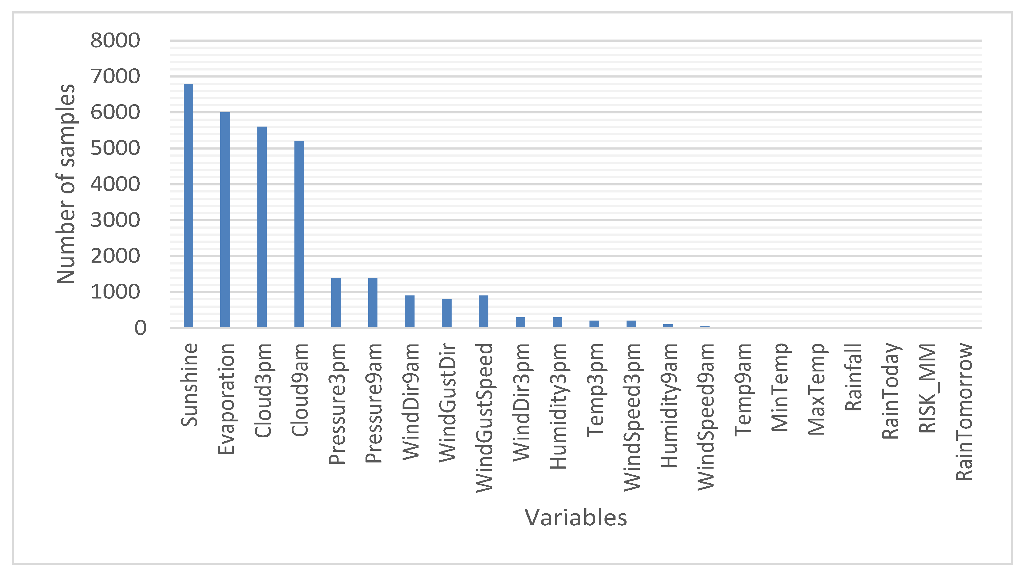
• Missing data. Figure 1 represents the number of samples of each of the variables for which there are no data. Thus, the total missing data correspond to 10% of the analyzed data (considering the total of 140,787 samples × 22 variables). Thus, if the samples that do not have data in any of their variables are eliminated, then approximately 50% of the samples would have to be eliminated. That is why the variables for which there are no data were analyzed, separating them by cities in order not to discard a large amount of data (the total number of cities for which data was available is 49). The results of the analysis of variables for which there are no data are as follows:
  • There are variables that do not have a single piece of data in some of the cities. It is considered that this is because the corresponding sensor does not exist in the meteorological station of that city. For this case, the absent values werewere replaced by the monthly average [35] of said variable considering all the cities.
  • There are samples for which there is no data for some of the variables. The reason could be a failure of the sensors or communication with them. Likewise, in this case, it was found that there are two different situations: data loss for one day only and data loss for several consecutive days. For this situation, it wasdecided to substitute the missing values for the monthly average [35] of said variable in the corresponding city.
  • Finally, in the case of the objective variable, RainToday, the decision was made to eliminate the samples in which the variable does not exist (an “NA” appears). In this sense, 1% of the data samples were deleted, leaving a total of 140,787 samples that contain a value other than “NA” in RainToday.
• Conversion of categorical variables to numeric. It was necessary to carry out this operation on two sets of variables. On the one hand, for the wind direction and for the Boolean, this indicates whether there is rain or not. In the first case, the variables that indicate the wind direction (WindGustDir, WindDir9am, and WindDir3pm) are of type “string” and must be transformed to be used. These variables can take 16 different directions, so that, in order to convert these values to real numbers, it must be taken into account that it presents a circular distribution. That is why each of the variables was split into two, one with the sine and the other with the cosine of the angle: WindGustDir_Sin, WindGustDir_Cos, WindDir9am_Sin, WindDir9am_Cos, WindDir3pm_Sin, and WindDir3pm_Cos. With respect to the second case, the variables of type “string” that represent Booleans (they take YES/NO) are transformed into the numerical values “1/0”.
• Elimination of variables. The date and location variables were eliminated, since they contain information that can be explained using other variables (the data corresponding to each location has not been separated to construct independent subsets, since the data in the region as a whole was to be studied). For example, there are cities that, depending on their locations, have humidity and temperature conditions that more or less favor rain. Likewise, on the date the data is obtained, different meteorological conditions may occur that influence the rain.
• Data normalization. A normalization of the data of the mix–max type [35] was carried out so that all the variables would take values between 0 and 1. In this way, variables taking values of great magnitudes having a greater influence on the application of machine learning algorithms was avoided.
• Detection of outliers. For this, the “Z-score” formula [36] was used, and all those samples that have Z > 3 were discarded. As a result, 7% of the data was removed from 140,787 samples to make 131,086.

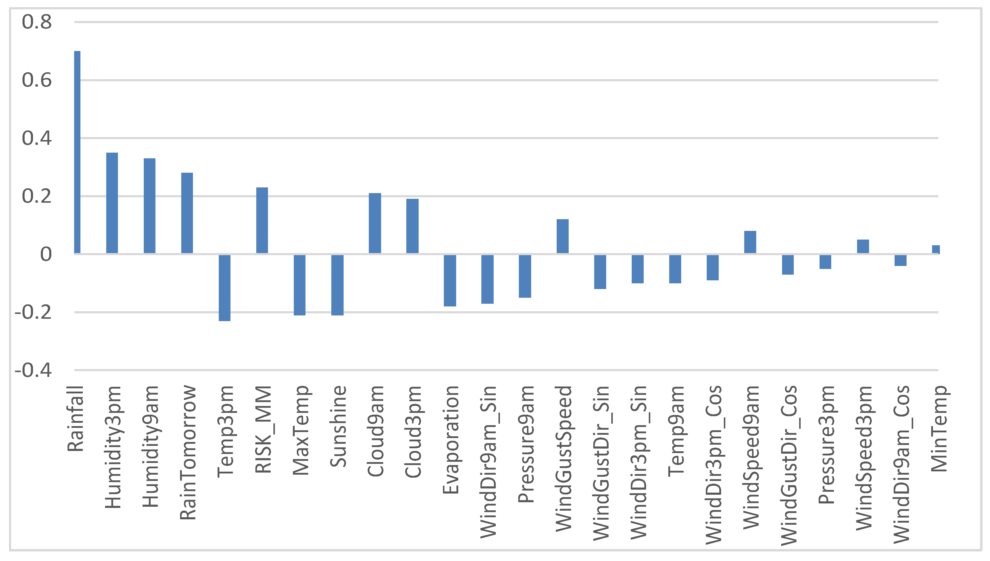
2.1.2. Correlation Analysis

Following the pre-processing of the data, a descriptive analysis of the variables was carried out in order to find out the form of the data to be analyzed. In particular, it was to carry out a study of the correlation that existed between the variable “RainToday” and the rest of the variables was studied. In Figure 2, the correlations appear ordered from highest to lowest according to their absolute values.

The following relationships with the variables can be observed (in those cases where the correlation value is greater than 0.2, it was decided to eliminate the variable):

• Rainfall: It is a variable that indicates the rain that has fallen (in mm), so it is a direct measure that indicates whether it has rained or not. For this reason, it was decided to eliminate rainfall from the set of variables to be used.
• RISK_MM: It is a variable that indicates the risk of rain. This variable was eliminated as it is not a measure of something physical since its value has probably been obtained by applying some non-detailed prediction model in the dataset.
• Humidity (Humidity3pm and Humidity9am). It is reasonable that they are related, since the higher the humidity, the greater the possibility of rain.
• Cloudiness (Cloud9am and Cloud3pm). It is reasonable that they are related because the greater the number of clouds, the more likely it is that it will rain more.
• In other variables, it is observed that there was an inverse relationship. So, by increasing the values of these variables, the possibility of rain is reduced. This happens with the variables Temp3pm and MaxTemp (an increase in temperature does not favor condensation) and Sunshine (an increase in radiation from the Sun would be directly related to a less cloudy day, and, therefore, there would be less rain).

2.1.3. Results of Data Preprocessing

The results of the data preprocessing is as follows:

• Initially there were 24 variables (‘Date’, ‘Location’, ‘MinTemp’, ‘MaxTemp’, ‘Rainfall’, ‘Evaporation’, ‘Sunshine’, ‘WindGustDir’, ‘WindGustSpeed’, ‘WindDir9am’, ‘WindDir3pm’, ‘WindSpeed9am’, ‘WindSpeed3pm’, ‘Humidity9am’, ‘Humidity3pm ’, ‘Pressure9am’, ‘Pressure3pm’, ‘Cloud9am’, ‘Cloud3pm’, ‘Temp9am’, ‘Temp3pm’, ‘RainToday’, ‘RISK_MM’, ‘RainTomorrow’) with a total of 142,193 samples corresponding to measurements of rainfall and atmospheric conditions produced in 49 cities in Australia over 10 years.
• The following variables were eliminated: Location/Date (eliminated because they are string variables), Rainfall (eliminated because they are highly related to the RainToday variable), RISK_MM (artificial variable obtained to predict the rain), RainTomorrow (removed because it is a variable artificial obtained from RISK_MM), and the variables WindGustDir, WindDir9am and WindDir3pm (each is split into two variables containing the cosines and sines of the wind direction angles).
• The samples that had “NA” in the RainToday variable were eliminated (it reduced the number from 142,193 samples to 140,787), and the samples that represent outliers were also eliminated (it reduced the number from 140,787 samples to 131,086)
• As a result, 21 variables were obtained (‘MinTemp’, ‘MaxTemp’, ‘Evaporation’, ‘Sunshine’, ‘WindGustSpeed’, ‘WindSpeed9am’, ‘WindSpeed3pm’, ‘Humidity9am’, ‘Humidity3pm’, ‘Pressure9am’, ‘Pressure3pm’, ‘Cloud9am’, ‘Cloud3pm’, ‘Temp9am’, ‘RainToday’, ‘Temp3pm’, ‘WindGustDir_Cos’, ‘WindGustDir_Sin’, ‘WindDir9am_Cos’, ‘WindDir9am_Sin’, ‘WindDir3pm_Cos’, ‘WindDir3pm_Sin’) with a total of 131,086 samples.

Note that of these 131,086 samples, 75% of the data is used to train the models with the different algorithms and the remaining 25% to check the effectiveness of these models.

2.2. Methods

The objective of this work is to analyze the possibilities offered by machine learning algorithms as tools for rain forecasting as an alternative to classical forecasting methods. For this, the following algorithms were applied: knn, decision tree, random forest, and neural networks. The algorithms are described below.

2.2.1. K-NN Algorithm (K-Nearest Neighbors)

It is a supervised algorithm (therefore, it takes labeled data as input) that for each unlabeled data sample identifies the K closest samples of the input data and assigns the class of most of the K closest neighbors to the unlabeled sample [37]. The algorithm requires the use of a function to calculate the distance between samples.

In theory, to choose the number K of closest samples to consider and avoid overfitting and underfitting [38], a bias–variance tradeoff is performed. It is a balance to reduce the impact of data with high variance and not ignore the trends generated by a small amount of data generating an offset (if a very high number is chosen for K, then the model would always predict the most common class, and if is a very small value was chosen this would generate a very noisy result). In practice [39], the selection of the value of K will depend on each case and the amount of data used to train the model. However, there are several widely used techniques, such as choosing the square root of the number of samples as a starting point and performing iterations considering different samples of training data, to be able to conclude on a suitable value of K or using a high value of K but appling a weight function to give more importance to the closest neighbors to the sample on which its class must be decided.

2.2.2. Decision Trees

It is an algorithm that uses a tree structure to model the relationships between variables [40]. The algorithm starts from an element called the root and is divided into increasingly narrow branches. Each division consists of making a decision and is represented by decision nodes. The process ends at leaf nodes that represent sufficiently homogeneous data that cannot be divided further.

One difficulty of this algorithm consists of identifying from which variable the division of the tree should be performed, for which it is necessary that the data contain a single class. To identify the best division candidate, two measures are used: entropy and the Gini index [41]. Entropy quantifies the randomness within a set of class values, such that sets with high entropy are very diverse and offer little information about other aspects that belong to the set. In this sense, the decision tree tends to find divisions that decrease entropy, increasing homogeneity within groups. On the other hand, the Gini index measures the probability that a variable is misclassified when it is taken randomly [42]. Its value varies between 0 (all the elements belong to a particular class or if there is only one class) and 1 (the elements are randomly distributed in different classes). Thus, a value of 0.5 would indicate that the elements are equally distributed in different classes. In this sense, when generating a decision tree, it is preferred to choose the variable with the smallest possible Gini index as the root element.

2.2.3. Random Forest

It is an algorithm that uses sets of decision trees that combine the principles of bagging (it consists of averaging many noisy models in order to reduce variation) with the random selection of features to add additional diversity to the decision tree models [43]. Once we have the set of decision trees generated, the model uses a vote to combine the predictions of the trees.

The main advantages of this algorithm are is the reduction of the possibility of over-fitting occurring [44], it allows eliminating variables that are not important, it can work with noisy or absent data, with continuous categorical or numerical variables, and with a number of variables or high samples. However, the main disadvantage is the difficulty of interpretation and visualization of the model [45].

2.2.4. Neural Networks

A neural network is an algorithm that models the relationship between a set of input values and a set of output values using a network of nodes called artificial neurons [46]. In the network, a weight is applied to each entry that represents its importance in the relationship. The inputs are then added, and a function called the activation function is applied to the result obtained, which transforms the combined inputs into an output. This function represents the way of processing and transmitting information through the network, different types of existing activation functions. In this sense, to select which one to use, the type of learning to be carried out, the limits of the functions (in X and Y), the variations of different functions, and the network architecture must be taken into account [47]. This last concept refers to the different ways of grouping neurons of the same type. In this sense, an architecture describes the number of neurons in the model, the number of layers, and the way they are interconnected. Each grouping is called a layer, and each architecture makes it possible to represent a set of data for which a model is to be obtained. There are three types of layers [48]: input (receive data), output (provide the network’s response to input), and hidden (do not receive or supply information and represent a type of internal network processing). On the other hand, according to the number of layers, neural networks can be classified as either a Single-layer network (a single input layer related to the output layer) or a multi-layer network (they have one or more layers between the inputs and the outputs and, in general, all the nodes of one layer are connected with all the nodes of the next layer). Generally, the connections are made between neurons of different layers, but there may be interlayer or lateral connections and feedback connections that follow a direction opposite to that of input–output. In this sense, according to the direction of the information in the neural network, they can be classified as either a [48] Feedforward network (unidirectional information flow) or a recurrent network (information flow in both directions using loops and delays. Finally, the learning algorithm in a network specifies how to apply the weights that depend on the learning paradigm (it depends on the information available to the network, so that it can be supervised if the expected output is known or unsupervised if the expected output is not known), the learning rules, and the type of learning algorithm (they can be based on error minimization, based on random parameters, based on competitive strategies, or based on Hebb’s law). Although the learning process (setting the weights) is complex, it has the advantage that, once learned, the network keeps the weights.

2.3. Key Performance Indicators

This section defines the metrics (or KPIs, Key Performance Indicators) used to be able to evaluate the results of the algorithms used [49]:

• Accuracy

Numeric value indicating the performance of the predictive model. It is calculated as follows:

$$\mathrm{Accuracy}=\frac{TP+TN}{TP+TN+FN+FP},$$

(1)

where:

• TP: True Positive. Result in which the model correctly predicts the positive class.
• FP: False Positive. Result in which the model incorrectly predicts the positive class.
• TN: True Negative. Result in which the model correctly predicts the negative class.
• FN: False Negative. Result in which the model incorrectly predicts the negative class.

2.

Kappa statistic

It measures the agreement between two examiners in their corresponding classifications of N elements into C mutually exclusive categories. In the case of machine learning, it refers to the actual class and the class expected by the model used. It is calculated as follows:

$$\mathrm{K}=\frac{\mathrm{Pr} \left(a\right)-\mathrm{Pr}\left(e\right)}{1-\mathrm{Pr}\left(e\right)},$$

(2)

where:

Pr (a) is the observed relative agreement between observers, and Pr (e) is the hypothesized probability of agreement by chance, using the observed data to compute the probabilities that each observer randomly ranks each category. If raters fully agree, then κ = 1. If there is no agreement between raters other than what would be expected by chance (as defined by Pr (e)), then κ = 0.

3.

Logarithmic Loss

It is the negative average of the log of corrected predicted probabilities for each instance. It is calculated as follows:

$$\mathrm{LogLoss}=\frac{-1}{N}{{\displaystyle \sum }}_{i=1}^N{{\displaystyle \sum }}_{j=1}^M{y}_{ij}·\log \left(p_{ij}\right),$$

(3)

where:

• N is the number of samples.
• M is the number of classes.
• y_ij, indicates if the sample i belongs to the class j or not.
• p_ij, indicates the probability that the sample i belongs to the class j.

4.

Error

The error gives an indication of how far the predictions are from the actual output. There are two formulas: Mean Absolute Error (MAE) and Mean Squared Error (MSE). It is calculated as follows:

$$\mathrm{MAE}=\frac{1}{N}{{\displaystyle \sum }}_{k=1}^N\left|y_k-\widehat{y_k}\right|$$

(4)

$$\mathrm{MSE}=\frac{1}{N}{{\displaystyle \sum }}_{j=1}^N{\left(y_k-\widehat{y_k}\right)}^2,$$

(5)

where:

• N corresponds to the total number of samples.
• $y_k$ corresponds to the class indicated by the classification model.
• $\widehat{y_k}$ corresponds to the actual class.

5.

Sensitivity

The sensitivity of a model (or the ratio of true positives) measures the proportion of correctly classified positive examples. The total number of positives is the sum of those that were correctly classified and those that were incorrectly classified. It is calculated as follows:

$$\mathrm{Sensitivity}=\frac{TP}{TP+FN },$$

(6)

where:

• TP: True Positive. Result in which the model correctly predicts the positive class.
• TN: True Negative. Result in which the model correctly predicts the negative class.
• FN: False Negative. Result in which the model incorrectly predicts the negative class.

6.

Specificity

The specificity of a model (or the ratio of true negatives) measures the proportion of correctly classified negative examples. The total number of negatives is the sum of those that were correctly classified and those that were incorrectly classified. It is calculated as follows:

$$\mathrm{Specificity}=\frac{TN}{TN+FP},$$

(7)

where:

• TP: True Positive. Result in which the model correctly predicts the positive class.
• FP: False Positive. Result in which the model incorrectly predicts the positive class.
• TN: True Negative. Result in which the model correctly predicts the negative class.

7.

Precision

Precision is defined as the proportion of examples classified as positive that are actually positive. That is, when a model predicts values as positive. It is calculated as follows:

$$\mathrm{Precision}=\frac{TP}{TP+FN},$$

(8)

where:

• TP: True Positive. Result in which the model correctly predicts the positive class.
• TN: True Negative. Result in which the model correctly predicts the negative class.
• FN: False Negative. Result in which the model incorrectly predicts the negative class.

8.

Recall

Recall is defined as the number of correctly classified positives over the total number of positives. This formula is the same as that for sensitivity. It is calculated as follows:

$$\mathrm{Recall}=\frac{TP}{TP+FP},$$

(9)

where:

• TP: True Positive. Result in which the model correctly predicts the positive class.
• FP: False Positive. Result in which the model incorrectly predicts the positive class.
• TN: True Negative. Result in which the model correctly predicts the negative class.

9.

F-measure

F-measure is a measure of model performance that combines precision and recall into a value called F-measure (also called F1 score or F-score). This measure combines precision and recall using harmonic averaging, which is used for ratios. This type of averaging is used instead of arithmetic, since precision and recall are expressed as proportions between 0 and 1, which can be interpreted as ratios. It is calculated as follows:

$$\mathrm{F}-\mathrm{measure}=\frac{2\ast precision\ast recall}{precision+recall}$$

(10)

3. Results

This section shows the result of applying different machine learning algorithms to the study data. The objective is to make the predictions of the variable “RainToday” from the database of rainfall in Australia. Each algorithm is discussed below.

3.1. KNN

This algorithm was implemented using the Python KNeighborsClassifier function defined in scikitlearn library [50]. The following parameters were modified:

-

n_neighbours. Number of neighbors to be used by the algorithm.

-

Weights.

• uniform’: all the points considered have an identical weight.
• distance’: a weight equal to the inverse of its distance from the point to be studied is assigned. That is, the closest neighbors will have a greater influence when deciding which class to assign the point to study.

For this algorithm the influence of different factors is analyzed:

• The impact of changing the value of the chosen K closest neighbors is checked. Using a “bias–variance trade-off” it was found that the optimal results are obtained for values between 20 and 30. Observe that the calculation time increases as the number of neighbors used to make the decision of the class to which the analyzed points belong increases.
• The impact of how the weights are assigned to the K closest neighbors is checked to decide the class that corresponds to it. With the default value, it was found that more values are classified as positive. However, the overall performance does not show that of the total points 0.7% is correctly classified as positive but 0.5% were incorrectly classified as negative. The calculation times are very similar to those obtained when using the “uniform” weight assignment instead of considering the inverse of the distance.

The most optimal combination of parameters for this algorithm were the following:

-

N_neighbors: 25.

-

Weights assignation: distance.

Table 2. Metrics evaluated for the KNN algorithm.

Accuracy	Error_Rate	Kappa	LogLoss	Sensitivity	Specificity	Precision	Recall	F1_Score
0.83	0.17	0.36	0.49	0.32	0.96	0.70	0.32	0.44

shows the results of the evaluated metrics.

3.2. Decision Tree

This algorithm was implemented using the Python DecisionTreeClassifier function defined in scikitLearn [51]. The following parameters were modified:

-

criterion: string.

• “entropy” for the information gain method.
• “gini” for the Gini impurity method.

-

splitter: string.

• “best” to choose the best partition.
• “random” to choose the best random partition.

-

max_depth: integral number indicating the greatest depth of the decision tree.

-

max_features: number of features to consider when looking for the best division.

-

random_state: corresponds to the seed used by the random number generator.

-

class_weight: weights associated with the classes; if no input is given, it is assumed that all classes have the same weight. The “balanced” option uses the value of each class to adjust the weights automatically, inversely proportional to the frequencies of each class in the data given as input.

For this algorithm the influence of different factors was analyzed:

• The impact of changing the number of max_depth was checked using the “entropy” criterion so that the optimal value was between 8 and 12. In this sense, 11 was chosen, making the best balance between the KPIs of accuracy, kappa, F1_score and error. Likewise, the impact of using the Gini information-gain criterion to perform the decision tree was verified, and the optimal numbers of tree levels match with those found when ordering according to the “entropy” criterion.

  Table 3. Metrics for max_depth parameter.

  Max_Depth	Accuracy	Error_Rate	Kappa	LogLoss	Sensitivity	Specificity	Precision	Recall	F1_Score
  Gini	0.83	0.17	0.41	0.8	0.44	0.93	0.61	0.44	0.51
  Entropy	0.83	0.17	0.42	1.02	0.45	0.92	0.61	0.45	0.52

  shows a comparison of the values obtained for the metrics considered according to the two criteria with a max_depth value of 11.
• The impact of changing the number of max_features (number of characteristics to consider when looking for the best division) in the results obtained was checked, setting the value of max_depth to 11 and using the entropy node division criterion. The best results were obtained if no restrictions were added to the characteristics.
• The impact of using the class_weight = “balanced” option was checked. To do this, the value of max_depth was set to 11, the entropy node division criterion was used, and a limit was not added for the max_features parameter. The weights were decided inversely proportionally to the number of these classes in the training data. As there was much less data assigned to class 1 (it does rain), this class was given much more importance, and, as a result, many values were assigned to the positive class (11,840 compared to 5090), increasing the number of TP from 3074 to 5121. At the same time, there was a significant increase in FP, from 2016 to 6719. Since the metrics obtained do not allow deciding the best value for the parameter, it was considered how many fewer false positives would be better to estimate if it rains or not, so the betterw option is “class_weight = balanced” than the default option.

  Table 4. Metrics for class_weight parameter.

  Class_Weight	Accuracy	Error_Rate	Kappa	LogLoss	Sensitivity	Specificity	Precision	Recall	F1_Score
  None	0.83	0.17	0.41	1.03	0.45	0.92	0.6	0.45	0.52
  Balanced	0.74	0.26	0.39	1.11	0.76	0.74	0.43	0.76	0.55

  shows the results of the evaluated metrics.
• The impact of using the splitter parameter was checked, so that the results were improved when it took the value of “best” instead of “random”, using the “entropy” classification criteria. The results are shown in

  Table 5. Metrics for splitter parameter.

  Splitter	Accuracy	Error_Rate	Kappa	LogLoss	Sensitivity	Specificity	Precision	Recall	F1_Score
  Best	0.83	0.17	0.42	1.02	0.46	0.92	0.61	0.46	0.52
  Random	0.82	0.18	0.35	0.73	0.35	0.95	0.63	0.35	0.45

  .
• The “Random state” parameter had no impact on the performance of the results obtained.

The most optimal combination of parameters for this algorithm were the following:

-

Max_depth: 11.

-

Max_features: 21 (the total of the features).

-

Class_weight: “Balanced”.

-

Criterion: “entropy”.

-

Splitter: “best”.

For this combination the values of

Table 6. Metrics evaluated for Decision Tree.

Accuracy	Error_Rate	Kappa	LogLoss	Sensitivity	Specificity	Precision	Recall	F1_Score
0.83	0.17	0.42	1.02	0.46	0.92	0.61	0.46	0.52

were obtained.

3.2.1. Random Forest

This algorithm was implemented using the Python RandomForestClassifier function defined in scikitLearn [52]. The following parameters were modified:

-

n_estimators: number of decision trees to consider.

-

criterion: string.

• “entropy” for the information gain method.
• “gini” for the Gini impurity method.

-

max_depth: integral number indicating the greatest depth of the decision tree.

-

class_weights: weights associated with the classes, if no input is given it is assumed that all classes have the same weight. The “balanced” option uses the values to adjust the weights automatically, inversely proportionally to the frequencies of each class in the data given as input.

For this algorithm the influence of different factors was analyzed:

• The impact of the max_depth parameter that indicates the depth of the tree was checked, so that it could be seen that for the “entropy” criterion the optimal parameter was 12, and for the “gini” criterion it was 13.

  Table 7. Metrics for splitter parameter.

  Max_Depth	Accuracy	Error_Rate	Kappa	LogLoss	Sensitivity	Specificity	Precision	Recall	F1_Score
  Entropy	0.84	0.16	0.45	0.37	0.44	0.95	0.68	0.44	0.54
  Gini	0.84	0.16	0.45	0.36	0.46	0.94	0.68	0.46	0.54

  shows the results for these parameter values.
• The impact of the number of estimators was checked using the “Gini” and “Entropy” criteria, so that the maximum precision was obtained when the number of estimators was 30, having reached very similar values of precision when the number of estimators was 10.
• The impact of using the class_weight = ”balanced” parameter to correct the weights according to the frequency of appearance of the different classes was verified. The results were compared with a case where the weights were not corrected. For this, 30 estimators were used, criterion = “entropy”, max_depth = 12 and max_features = 21. In conclusion, it was found that the results obtained improved (the impact of modifying the weights was inversely proportional to the number of elements in the class was greater than when the standard decision tree check was performed). The result is shown in

  Table 8. Metrics for class_weight parameter.

  Class_Weight	Accuracy	Error_Rate	Kappa	LogLoss	Sensitivity	Specificity	Precision	Recall	F1_Score
  None	0.85	0.15	0.45	0.35	0.44	0.95	0.7	0.44	0.54
  Balanced	0.81	0.19	0.49	0.41	0.71	0.84	0.53	0.71	0.61

  .
• In RandomForest each tree in the set was created from a sample with replacement of the training dataset. Furthermore, when each node was separated construct a decision tree, the best split was found from all features or from a random set of size “max_features”.

The most optimal combination of parameters for this algorithm was the following:

-

N_estimators: 30.

-

Max_depth: 14.

-

Max_features: 21 (the total of the features).

-

Criterion: “gini”.

-

class_weight = ”balanced”.

For this combination the values of

Table 9. Metrics evaluated for Random Forest.

Accuracy	Error_Rate	Kappa	LogLoss	Sensitivity	Specificity	Precision	Recall	F1_Score
0.83	0.17	0.5	0.39	0.66	0.87	0.57	0.66	0.61

are obtained.

3.2.2. Neural Networks

This algorithm was implemented using the Python MLPClassifier function defined in scikitLearn [53]. The following parameters were modified:

-

Hidden_layer_sizes: tuple, length = n_layers-2, default (100). The element i represents the number of neurons in the hidden layer i.

-

Activation: Activation function for hidden layers. Can be:

• ‘identity’: no-op activation, useful to implement linear bottleneck, f (x) = x.
• ‘logistic’: sigmoid activation function.
• ‘tanh’, hyperbolic tangent function.
• ‘relu’, rectified linear function.

-

solver: Solver used for the optimization of the weights.

• ‘lbfgs’ optimizer family of quasi-Newtonian methods.
• ‘sgd’ stochastic gradient descent optimizer.
• ‘adam’ referring to a gradient-based stochastic optimizer.

-

alpha: regularization parameter L2 penalty. It helps to avoid overfitting by penalizing the weights with high magnitudes.

For this algorithm the influence of different factors was analyzed:

• The impact of changing the activation function was verified so that the best results were obtained for the “relu” function, as shown in

  Table 10. Metrics for activation parameter.

  Activation	Accuracy	Error_Rate	Kappa	LogLoss	Sensitivity	Specificity	Precision	Recall	F1_Score
  identity	0.83	0.17	0.4	0.37	0.39	0.95	0.66	0.39	0.49
  logistic	0.84	0.16	0.42	0.36	0.42	0.95	0.67	0.42	0.51
  tanh	0.84	0.16	0.46	0.35	0.46	0.94	0.68	0.46	0.55
  relu	0.85	0.15	0.47	0.35	0.47	0.95	0.69	0.47	0.56

  .
• The impact of the solver parameter (optimization of the weights) used to solve the algorithm weights was checked so that the best results were obtained for the “adam” function as shown in

  Table 11. Metrics for solver parameter.

  Solver	Accuracy	Error_Rate	Kappa	LogLoss	Sensitivity	Specificity	Precision	Recall	F1_Score
  Ibfgs	0.85	0.15	0.47	0.35	0.47	0.95	0.69	0.47	0.56
  Sgd	0.84	0.16	0.43	0.36	0.43	0.94	0.67	0.43	0.52
  adam	0.85	0.15	0.49	0.34	0.51	0.93	0.66	0.51	0.58

  .
• The impact of changing the alpha parameter was verified (it helps to avoid overfitting by penalizing weights with high magnitudes) so that the optimum was obtained at 0.05.

The most optimal combination of parameters for this algorithm was the following:

-

Activation = ‘relu’.

-

Solver = ‘adam’.

-

Alpha = 0.05.

For this combination the values of

Table 12. Metrics evaluated for Neural Network.

Accuracy	Error_Rate	Kappa	LogLoss	Sensitivity	Specificity	Precision	Recall	F1_Score
0.84	0.16	0.49	0.35	0.53	0.92	0.65	0.53	0.59

are obtained.

4. Discussion

The models described were compared to analyze which one best predicts the target variable. In this sense,

Table 13. Model comparison.

Algorithm	Misclassification Rate	MSE	AUC
K-NN	0.044	0.042	0.5
Decision tree	0.044	0.043	0.6
Random forest	0.044	0.041	0.65
Neural network	0.044	0.039	0.7

shows the rate of classification errors, the MSE, and the AUC for each model studied.

The misclassification rate is the same for all models, so the other metrics were used. If the AUC is considered, it is observed that the model that has a higher value is neural networks. In the same way, if the MSE is considered, it is found that the lowest value is also obtained with the neural network model. The result was validated by performing cross-validation and rebuilding the models. The analysis shows the same results, which may be due to overfitting or a very homogeneous sample. In this sense, it was studied whether there was an overfitting. For this, the results obtained in the training and test sets were taken in order to verify if the training results were very good (overfit) and if the results worsened significantly in the test. The results show that there was no data overfitting, since they were numerically similar. This allows me to conclude that the cause of these results was the homogeneity of the data.

Therefore, the results of this research show that the best result is obtained with the neural network model with activation function “tanh”, algorithm “adam”, and value 0.05 for alpha. The results are consistent with the results obtained by the authors cited in the introduction [28,29,30,31,32,33,34] and show that it is a non-linear phenomenon. This aspect explains the fact that neural networks are the best model to describe it, since they behave very well with this type of phenomenon. For this reason, the use of more advanced neural networks will probably allow me to obtain better results.

Moreover, the impact of the data used to train and check the model was studied. For this, it changed the input data from the Python function train_test_split used to prepare the data. Firstly, the amount of data used to train the model varied, and the results show that it has a negligible impact on the quality of the models. The function’s “random_state” parameter used to separate the training data from the data used to test the algorithm was modified. In addition, no effect was found on the results of the accuracy of the algorithm obtained.

Finally, the effect of the locality of the data was studied. In the previous study, a dataset with a large number of cities was used. In addition, in some cases, there are variables for which data do not exist and it was necessary to make estimates. For this reason, the cities that have the most variables with data (i.e., Sydney, Perth, and Darwin) were considered, and the accuracy of the predictive models based on Random Forest and Neural Networks applied independently to each city was analyzed.

(a)

City of Sydney

Parameters used in Random Forest:

-

Max_depth = 9.

-

Criterion = “gini”.

-

Class_weight = ‘balanced’.

-

N_estimators = 20.

Parameters used in Neural Network:

-

Activation = ‘relu’.

-

Solver = ‘lbfgs’.

-

Alpha = 0.0025.

The results are shown in

Table 14. Models for city of Sydney.

Algorithm	Accuracy	Error_Rate	Kappa	LogLoss	Sensitivity	Specificity	Precision	Recall	F1_Score
Random Forest	0.84	0.16	0.51	0.42	0.59	0.91	0.64	0.59	0.62
Neural network	0.84	0.16	0.52	0.44	0.57	0.92	0.67	0.57	0.62

.

(b)

City of Perth

Parameters used in Random Forest:

-

Max_depth = 8.

-

Criterion = ‘gini’.

-

Class_weight = ‘balanced’.

-

N_estimators = 18.

Parameters used in Neural Network (NN):

-

Activation = ‘relu’.

-

Solver = ‘adam’.

-

Alpha = 0.025.

The results are shown in

Table 15. Models for city of Perth.

Algorithm	Accuracy	Error_Rate	Kappa	LogLoss	Sensitivity	Specificity	Precision	Recall	F1_Score
Random Forest	0.9	0.1	0.7	0.3	0.83	0.92	0.7	0.83	0.76
Neural network	0.93	0.07	0.77	0.2	0.78	0.97	0.85	0.78	0.81

.

(c)

City of Darwin

Parameters used in R.Forest:

-

Max_depth = 9.

-

Criterion = “gini”.

-

Class_weight = ‘balanced’.

-

N_estimators = 36.

Parameters used in Neural Network (NN):

-

Activation = ‘identity’.

-

Solver = ‘lbfgs’.

-

Alpha = 0.1.

The results are shown in

Table 16. Models for city of Darwin.

Algorithm	Accuracy	Error_Rate	Kappa	LogLoss	Sensitivity	Specificity	Precision	Recall	F1_Score
Random Forest	0.88	0.12	0.61	0.31	0.65	0.94	0.72	0.65	0.68
Neural network	0.88	0.12	0.6	0.31	0.62	0.94	0.74	0.62	0.67

.

As can be seen, an improvement in the accuracy of the predictive models is obtained by making models for the different cities independently, obtaining the best values for the city of Perth.

5. Conclusions and Future Work

In this work, the applicability of machine learning techniques to the problem of rainfall forecasting in the specific case of Australia was studied. There are previous works [28,29,30,31,32,33,34] that have applied this type of technique in regions other than Australia and with different types of monthly, annual, and other time period datasets. The locations that were studied were the regions of Victoria and Sydney, and the models used were, generally, Neural Networks and Random Forest. In line with these previous studies, in this work, a set of meteorological data from 49 different cities in Australia was taken. In the set, there is a variable (RainToday) that indicates whether or not it has rained on the day of taking the sample, and there are also other variables that show meteorological properties on the day of taking the sample, such as cloudiness, wind, sunlight, humidity, pressure, or temperature. From the preprocessed dataset, several prediction models based on machine learning techniques were applied to predict rainfall (Knn, Decision Tree, Random Forest, and Neural Networks). As a result, it was found that the best model to describe this type of phenomenon is neural networks. Likewise, the applicability of the models to various cities was analyzed independently. In this case, it was observed that the efficiency of the algorithms was higher. Finally, the possible improvement of the results by modifying the data used to carry out the training (quantity of data and actual values) was studied but without improvement compared with previous analyses. Therefore, this new study allowed me to conclude several ideas. On the one hand, the possibilities offered by machine learning techniques as alternative tools to classical rain forecasting methods (they also have some advantages over classical forecasting methods, such as the possibility of estimating the reliability of the results using the Indicators, Performance Key, or the possibility of adjusting the performance of the algorithms by manipulating their input parameters, which allows them to be adapted to particular cases). Likewise, it can be seen that algorithms based on Neural Networks work quite well to model nonlinear natural phenomena. Finally, the locality of the phenomenon can be observed, since, by considering the data independently by city, the algorithms work and are more efficient.

The work can be continued in several ways. Thus, it would be interesting to check the results obtained considering the meteorological information from 2019 to the present, as well as the analysis of data from other countries. The latter would allow me to check whether the efficiency obtained can be extrapolated to other geographical areas and there is no geographical dependence on the results. Finally, another very interesting future study related to the one described would be to study the problem of predicting, several days in advance, which models are the most interesting or how many days in advance are optimal for making a prediction.

References

- Datta, A.; Si, S.; Biswas, S. Complete Statistical Analysis to Weather Forecasting. In Computational Intelligence in Pattern Recognition; Springer: Singapore, 2020; pp. 751–763. [Google Scholar]
- Burlando, P.; Montanari, A.; Ranzi, R. Forecasting of storm rainfall by combined use of radar, rain gages and linear models. Atmos. Res. 1996, 42, 199–216. [Google Scholar] [CrossRef]
- Valipour, M. How much meteorological information is necessary to achieve reliable accuracy for rainfall estimations? Agriculture 2016, 6, 53. [Google Scholar] [CrossRef] [Green Version]
- Murphy, A.H.; Winkler, R.L. Probability forecasting in meteorology. J. Am. Stat. Assoc. 1984, 79, 489–500. [Google Scholar] [CrossRef]
- Jolliffe, I.T.; Stephenson, D.B. (Eds.) Forecast Verification: A Practitioner’s Guide in Atmospheric Science; John Wiley & Sons: Hoboken, NJ, USA, 2012. [Google Scholar]
- Wu, J.; Huang, L.; Pan, X. A novel bayesian additive regression trees ensemble model based on linear regression and nonlinear regression for torrential rain forecasting. In Proceedings of the 2010 Third International Joint Conference on Computational Science and Optimization, Huangshan, China, 28–31 May 2010; Volume 2, pp. 466–470. [Google Scholar]
- Tanessong, R.S.; Vondou, D.A.; Igri, P.M.; Kamga, F.M. Bayesian processor of output for probabilistic quantitative precipitation forecast over central and West Africa. Atmos. Clim. Sci. 2017, 7, 263. [Google Scholar] [CrossRef] [Green Version]
- Georgakakos, K.P.; Hudlow, M.D. Quantitative precipitation forecast techniques for use in hydrologic forecasting. Bull. Am. Meteorol. Soc. 1984, 65, 1186–1200. [Google Scholar] [CrossRef]
- Migon, H.S.; Monteiro, A.B.S. Rain-fall modeling: An application of Bayesian forecasting. Stoch. Hydrol. Hydraul. 1997, 11, 115–127. [Google Scholar] [CrossRef]
- Wu, J. An effective hybrid semi-parametric regression strategy for rainfall forecasting combining linear and nonlinear regression. In Modeling Applications and Theoretical Innovations in Interdisciplinary Evolutionary Computation; IGI Global: New York, NY, USA, 2013; pp. 273–289. [Google Scholar]
- Wu, J. A novel nonlinear ensemble rainfall forecasting model incorporating linear and nonlinear regression. In Proceedings of the 2008 Fourth International Conference on Natural Computation, Jinan, China, 18–20 October 2008; Volume 3, pp. 34–38. [Google Scholar]
- Zhang, C.J.; Zeng, J.; Wang, H.Y.; Ma, L.M.; Chu, H. Correction model for rainfall forecasts using the LSTM with multiple meteorological factors. Meteorol. Appl. 2020, 27, e1852. [Google Scholar] [CrossRef] [Green Version]
- Liguori, S.; Rico-Ramirez, M.A.; Schellart, A.N.A.; Saul, A.J. Using probabilistic radar rainfall nowcasts and NWP forecasts for flow prediction in urban catchments. Atmos. Res. 2012, 103, 80–95. [Google Scholar] [CrossRef]
- Koussis, A.D.; Lagouvardos, K.; Mazi, K.; Kotroni, V.; Sitzmann, D.; Lang, J.; Malguzzi, P. Flood forecasts for urban basin with integrated hydro-meteorological model. J. Hydrol. Eng. 2003, 8, 1–11. [Google Scholar] [CrossRef]
- Yasar, A.; Bilgili, M.; Simsek, E. Water demand forecasting based on stepwise multiple nonlinear regression analysis. Arab. J. Sci. Eng. 2012, 37, 2333–2341. [Google Scholar] [CrossRef]
- Holmstrom, M.; Liu, D.; Vo, C. Machine learning applied to weather forecasting. Meteorol. Appl. 2016, 10, 1–5. [Google Scholar]
- Singh, N.; Chaturvedi, S.; Akhter, S. Weather forecasting using machine learning algorithm. In Proceedings of the 2019 International Conference on Signal Processing and Communication (ICSC), Noida, India, 7–9 March 2019; pp. 171–174. [Google Scholar]
- Hasan, N.; Uddin, M.T.; Chowdhury, N.K. Automated weather event analysis with machine learning. In Proceedings of the 2016 International Conference on Innovations in Science, Engineering and Technology (ICISET), Dhaka, Bangladesh, 28–29 October 2016; pp. 1–5. [Google Scholar]
- Balamurugan, M.S.; Manojkumar, R. Study of short term rain forecasting using machine learning based approach. Wirel. Netw. 2021, 27, 5429–5434. [Google Scholar] [CrossRef]
- Booz, J.; Yu, W.; Xu, G.; Griffith, D.; Golmie, N. A deep learning-based weather forecast system for data volume and recency analysis. In Proceedings of the 2019 International Conference on Computing, Networking and Communications (ICNC), Honolulu, HI, USA, 18–21 February 2019; pp. 697–701. [Google Scholar]
- Liu, J.N.; Lee, R.S. Rainfall forecasting from multiple point sources using neural networks. In Proceedings of the IEEE SMC’99 Conference Proceedings. 1999 IEEE International Conference on Systems, Man, and Cybernetics (Cat. No. 99CH37028), Tokyo, Japan, 12–15 October 1999; Volume 3, pp. 429–434. [Google Scholar]
- Darji, M.P.; Dabhi, V.K.; Prajapati, H.B. Rainfall forecasting using neural network: A survey. In Proceedings of the 2015 International Conference on Advances in Computer Engineering and Applications, IEEE, Ghaziabad, India, 19–20 March 2015; pp. 706–713. [Google Scholar]
- Mahabub, A.; Habib, A.Z.S.B.; Mondal, M.; Bharati, S.; Podder, P. Effectiveness of ensemble machine learning algorithms in weather forecasting of bangladesh. In Proceedings of the International Conference on Innovations in Bio-Inspired Computing and Applications, online, 16–18 December 2020; Springer: Cham, Switzerland, 2020; pp. 267–277. [Google Scholar]
- Rizvee, M.A.; Arju, A.R.; Al-Hasan, M.; Tareque, S.M.; Hasan, M.Z. Weather Forecasting for the North-Western region of Bangladesh: A Machine Learning Approach. In Proceedings of the 2020 11th International Conference on Computing, Communication and Networking Technologies (ICCCNT), Kharagpur, India, 1–3 July 2020; pp. 1–6. [Google Scholar]
- Bushara, N.O.; Abraham, A. Weather forecasting in Sudan using machine learning schemes. J. Netw. Innov. Comput. 2014, 2, 309–317. [Google Scholar]
- Ingsrisawang, L.; Ingsriswang, S.; Somchit, S.; Aungsuratana, P.; Khantiyanan, W. Machine learning techniques for short-term rain forecasting system in the northeastern part of Thailand. Proc. World Acad. Sci. Eng. Technol. 2008, 31, 248–253. [Google Scholar]
- Macabiog, R.E.N.; Cruz, J.C.D. Rainfall Predictive Approach for La Trinidad, Benguet using Machine Learning Classification. In Proceedings of the 2019 IEEE 11th International Conference on Humanoid, Nanotechnology, Information Technology, Communication and Control, Environment, and Management (HNICEM), Laoag, Philippines, 29 November–1 December 2019; pp. 1–6. [Google Scholar]
- Pham, Q.B.; Kumar, M.; Di Nunno, F.; Elbeltagi, A.; Granata, F.; Islam, A.R.M.; Anh, D.T. Groundwater level prediction using machine learning algorithms in a drought-prone area. Neural Comput. Appl. 2022, 17, 1–23. [Google Scholar] [CrossRef]
- Bagirov, A.M.; Mahmood, A.; Barton, A. Prediction of monthly rainfall in Victoria, Australia: Clusterwise linear regression approach. Atmos. Res. 2017, 188, 20–29. [Google Scholar] [CrossRef]
- Granata, F.; Di Nunno, F. Forecasting evapotranspiration in different climates using ensembles of recurrent neural networks. Agric. Water Manag. 2021, 255, 107040. [Google Scholar] [CrossRef]
- Sachindra, D.A.; Ahmed, K.; Rashid, M.M.; Shahid, S.; Perera, B.J.C. Statistical downscaling of precipitation using machine learning techniques. Atmos. Res. 2018, 212, 240–258. [Google Scholar] [CrossRef]
- Raval, M.; Sivashanmugam, P.; Pham, V.; Gohel, H.; Kaushik, A.; Wan, Y. Automated predictive analytics tool for rainfall forecasting. Sci. Rep. 2021, 11, 17704. [Google Scholar] [CrossRef]
- Feng, P.; Wang, B.; Li Liu, D.; Ji, F.; Niu, X.; Ruan, H.; Yu, Q. Machine learning-based integration of large-scale climate drivers can improve the forecast of seasonal rainfall probability in Australia. Environ. Res. Lett. 2020, 15, 084051. [Google Scholar] [CrossRef]
- Hartigan, J.; MacNamara, S.; Leslie, L.M.; Speer, M. Attribution and prediction of precipitation and temperature trends within the Sydney catchment using machine learning. Climate 2020, 8, 120. [Google Scholar] [CrossRef]
- Taylor, J.K.; Cihon, C. Statistical Techniques for Data Analysis; CRC Press: Boca Raton, FL, USA, 2004. [Google Scholar]
- Somasundaram, R.S.; Nedunchezhian, R. Evaluation of three simple imputation methods for enhancing preprocessing of data with missing values. Int. J. Comput. Appl. 2011, 21, 14–19. [Google Scholar] [CrossRef]
- Zhang, S.; Cheng, D.; Deng, Z.; Zong, M.; Deng, X. A novel kNN algorithm with data-driven k parameter computation. Pattern Recognit. Lett. 2018, 109, 44–54. [Google Scholar] [CrossRef]
- Deng, Z.; Zhu, X.; Cheng, D.; Zong, M.; Zhang, S. Efficient kNN classification algorithm for big data. Neurocomputing 2016, 195, 143–148. [Google Scholar] [CrossRef]
- Pandey, A.; Jain, A. Comparative analysis of KNN algorithm using various normalization techniques. Int. J. Comput. Netw. Inf. Secur. 2017, 9, 36. [Google Scholar] [CrossRef] [Green Version]
- Patel, H.H.; Prajapati, P. Study and analysis of decision tree based classification algorithms. Int. J. Comput. Sci. Eng. 2018, 6, 74–78. [Google Scholar] [CrossRef]
- Rao, H.; Shi, X.; Rodrigue, A.K.; Feng, J.; Xia, Y.; Elhoseny, M.; Yuan, X.; Gu, L. Feature selection based on artificial bee colony and gradient boosting decision tree. Appl. Soft Comput. 2019, 74, 634–642. [Google Scholar] [CrossRef]
- Fiarni, C.; Sipayung, E.M.; Tumundo, P.B. Academic decision support system for choosing information systems sub majors programs using decision tree algorithm. J. Inf. Syst. Eng. Bus. Intell. 2019, 5, 57–66. [Google Scholar] [CrossRef] [Green Version]
- Schonlau, M.; Zou, R.Y. The random forest algorithm for statistical learning. Stata J. 2020, 20, 3–29. [Google Scholar] [CrossRef]
- Probst, P.; Wright, M.N.; Boulesteix, A.L. Hyperparameters and tuning strategies for random forest. Wiley Interdiscip. Rev. Data Min. Knowl. Discov. 2019, 9, e1301. [Google Scholar] [CrossRef] [Green Version]
- Tyralis, H.; Papacharalampous, G.; Langousis, A. A brief review of random forests for water scientists and practitioners and their recent history in water resources. Water 2019, 11, 910. [Google Scholar] [CrossRef] [Green Version]
- Wu, Y.C.; Feng, J.W. Development and application of artificial neural network. Wirel. Pers. Commun. 2018, 102, 1645–1656. [Google Scholar] [CrossRef]
- Abiodun, O.I.; Jantan, A.; Omolara, A.E.; Dada, K.V.; Mohamed, N.A.; Arshad, H. State-of-the-art in artificial neural network applications: A survey. Heliyon 2018, 4, e00938. [Google Scholar] [CrossRef] [PubMed] [Green Version]
- Blalock, D.; Gonzalez Ortiz, J.J.; Frankle, J.; Guttag, J. What is the state of neural network pruning? Proc. Mach. Learn. Syst. 2020, 2, 129–146. [Google Scholar]
- Badawy, M.; Abd El-Aziz, A.A.; Idress, A.M.; Hefny, H.; Hossam, S. A survey on exploring key performance indicators. Future Comput. Inform. J. 2016, 1, 47–52. [Google Scholar] [CrossRef]
- KNeighborsClassifier Function. Available online: https://scikitlearn.org/stable/modules/generated/sklearn.neighbors.KNeighborsClassifier.html#sklearn.neighbors.KNeighboursClassifier (accessed on 17 February 2022).
- DecisionTreeClassifier Function. Available online: https://scikit-learn.org/stable/modules/generated/sklearn.tree.DecisionTreeClassifier.html (accessed on 17 February 2022).
- RandomForestClassifier Function. Available online: https://scikit-learn.org/stable/modules/generated/sklearn.ensemble.RandomForestClassifier.html (accessed on 17 February 2022).
- MLPClassifier Function. Available online: https://scikit-learn.org/stable/modules/generated/sklearn.neural_network.MLPClassifier.html (accessed on 17 February 2022).