Abstract
Canonical Correlation Analysis (CCA) is a classic multivariate statistical technique, which can be used to find a projection pair that maximally captures the correlation between two sets of random variables. The present paper introduces a CCA-based approach for image retrieval. It capitalizes on feature maps induced by two images under comparison through a pre-trained Convolutional Neural Network (CNN) and leverages basis vectors identified through CCA, together with an element-wise selection method based on a Chernoff-information-related criterion, to produce compact transformed image features; a binary hypothesis test regarding the joint distribution of transformed feature pair is then employed to measure the similarity between two images. The proposed approach is benchmarked against two alternative statistical methods, Linear Discriminant Analysis (LDA) and Principal Component Analysis with whitening (PCAw). Our CCA-based approach is shown to achieve highly competitive retrieval performances on standard datasets, which include, among others, Oxford5k and Paris6k.
1. Introduction
The past two decades have witnessed an explosive growth of online image databases. This growth paves the way for the development of visual-data-driven applications, but at the same time poses a major challenge to the Content-Based Image Retrieval (CBIR) technology [1].
Traditional approaches to CBIR mostly rely on the exploitation of handrafted scale- and orientation-invariant image features [2,3,4,5,6], which have achieved varying degrees of success. Recent advances [7,8] in Deep Learning (DL) for image classification and object detection have generated significant interests in bringing Convolutional Neural Networks (CNNs) to bear upon CBIR. Although CNN models are usually trained for purposes different from CBIR, it is known [9] that features extracted from modern deep CNNs, commonly referred to as DL features, have great potential in this respect as well. Retrieval methods utilizing DL features can generally be divided into two categories: without/with fine-tuning the CNN model [10]. The early application of CNN to CBIR almost exclusively resorts to methods in the first category, which use Off-The-Shelf (OTS) CNNs (i.e., popular pre-trained CNNs) for feature extraction (see, e.g., [11,12,13,14]). A main advantage of such methods is the low implementation cost [15,16], which is largely attributed to the direct adoption of pre-trained CNNs. Performance-wise, they are comparable to the state-of-the-art traditional methods that rely on handcrafted features. In contrast, many recent methods, such as [17,18,19], belong to the second category, which take advantage of the fine-tuning gain to enhance the discriminatory power of the extracted DL features. A top representative from this category is the end-to-end learning framework proposed in [20]. It outperforms most existing traditional and OTS-CNN-based methods on standard testing datasets; however, this performance improvement comes at the cost of training a complex triple-branched CNN using a large dataset, which might not always be affordable in practice.
Many preprocessing methods have been developed with the goal of better utilizing DL features for image retrieval, among which Principal Component Analysis with whitening [21] (PCAw) and Linear Discriminant Analysis [22] (LDA) are arguably most well known. Despite being extremely popular, PCA and LDA have their respective weaknesses: the dimensionality reduction in PCA often leads to the elimination of critical principal components with a small contribution rate while the performance of LDA tends to suffer from decreasing differences between mismatched features. As such, there is great need for a preprocessing method with improved robustness against dimensionality reduction and enhanced sensitivity to feature mismatch. In this work, we aim to put forward a potential solution with desired properties by bringing Canonical Correlation Analysis (CCA) [23] into the picture.
CCA is a multivariate technique for elucidating the the associations among two sets of variables. It can be used to identify a projection pair of a given dimension that maximally captures the correlation between the two sets. The applications of CCA are too numerous to list. In cross-modality matching/retrieval alone, extensive investigations have been carried out as evidenced by a growing body of literature, from those based on handcrafted features [24] to the more recent ones that make use of DL features [25,26,27]. There is also some related development on the theoretical front (see, e.g., [28,29]).
Motivated by the consideration of computational efficiency and affordability as well as the weaknesses inherent in the existing preprocessing methods, we develop and present in this paper a new image retrieval method based on OTS deep CNNs. Our method is built primarily upon CCA, but has several notable differences from the related works. For the purpose of dimensionality reduction (i.e., feature compression), the proposed method employs a basis-vector selection technique, which invokes a Chernoff-information-based criterion to rank how discriminative the basis vectors are. Both the basis vectors and their ranking are learned from a training set, which consists of features extracted from a pre-trained CNN—the neural network itself is not retrained/finetuned in our work. Given a new pair of features, the ranked basis vectors are used to perform transformation and compression. This is followed by a binary hypothesis test on the joint distribution of pairs of transformed features, which yields a matching score that can be leveraged to identify top candidates for retrieval. We show via extensive experimental results that the proposed CCA-based method is able to deliver highly competitive results on standard datasets, which include, among others, Oxford5k and Parise6k.
2. Proposed Method
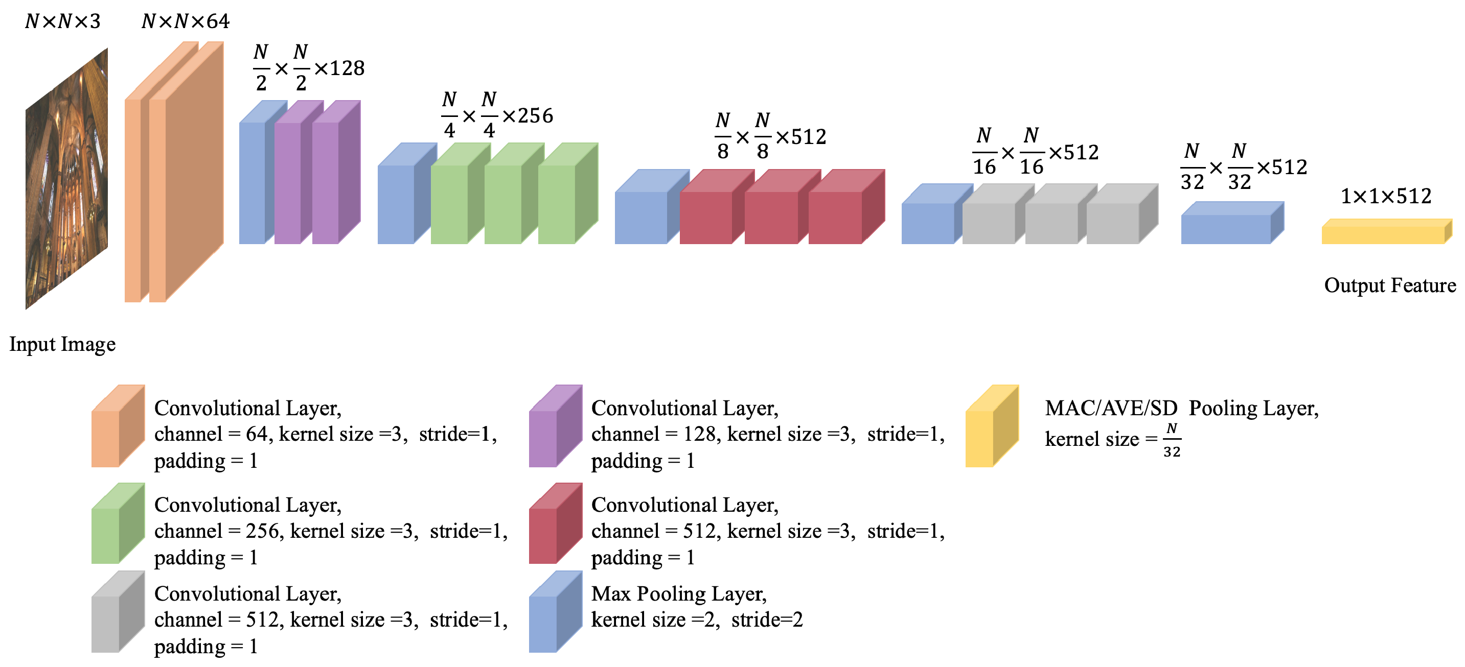
The proposed image retrieval method utilizes CCA in an essential way. It leverages a training dataset of features extracted from a pre-trained CNN model (see Figure 1) to learn a set of canonical vectors, which serve as the basis vectors of the feature space. These vectors are used to project the features of a pair of images into a new space, in which a Chernoff-information-based selection method is applied to identify the most discriminative elements of the transformed features. Such elements then undergo a binary hypothesis test to measure the similarity between the features and, consequently, the two images. This process is expounded in the following four subsections (see also Figure 2).
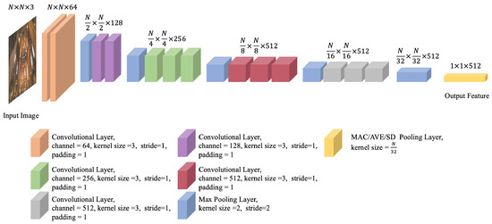
Figure 1.
Modified VGG16 for feature extraction.
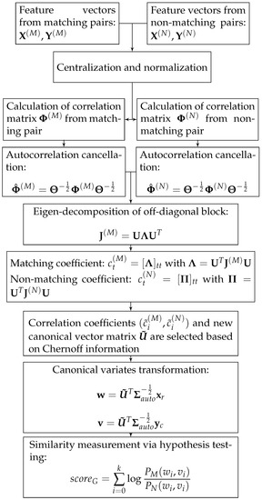
Figure 2.
Block diagram of the proposed method.
2.1. Image Pre-Processing and Feature Extraction
The CNN model adopted in this work for feature extraction is VGG16 [30]. It takes an input image of maximum size and produces 512 feature maps of maximum size from its very last pooling layer. A single feature element is extracted from each feature map via pooling. A 512-dimensional vector, which resulted from the concatenation of these elements, is converted, through centralization and normalization (here centralization is performed by subtracting the mean (computed based on the training set) while normalization yields a unit-length vector), to a global feature vector, which serves as a compact representation of the image.
2.2. Correlation Analysis and Canonical Vectors
At the heart of the proposed method lies so-called canonical vectors, which are learned from a large training set of matching and non-matching image features in a manner inspired by CCA. The learning process consists of the following steps.
Step 1: Construct two raw matching matrices
where L is the number of raw matching pairs, and for are a pair of global feature vectors representing two matching images (here “matching images” means images from the same class while “non-matching images” means images from different classes).
Using the raw matching pairs and , a pair of matching-feature matrices is formed:
The total number of training pairs is after feature order flipped. This is performed to ensure that in Equation (1) below, the diagonal blocks are identical and symmetric, so are the off-diagonal blocks. The size of both and is . The training data matrix of matching features is constructed by stacking on :
The estimated covariance matrix of matching features is given by
where
Step 2: Randomly permuting the columns of one of the raw feature matrices, say from to , yields two raw non-matching matrices. More specifically, we construct two raw non-matching matrices by successively associating each column of with a randomly selected (without replacement) non-matching column from . For example,
Based on these two raw non-matching matrices, the feature order flipping is performed to generate and :
With a procedure similar to that of step 1, we can estimate the covariance matrix for non-matching features :
Note that
for they are the covariances of sets of random image features. As in Equation (1), the diagonal blocks in Equation (2) are also identical and symmetric, so are the off-diagonal blocks.
Step 3: Since is positive definite, it follows that is well defined, where
We can multiply both covariance matrices, and , on the left and right by to de-correlate their diagonal blocks:
where
Step 4: Apply eigen-decomposition [31] on :
where is a unitary matrix, and is a diagonal matrix with the diagonal entries being the eigenvalues of . The columns of are exactly the sought-after canonical vectors. The blockwise left- and right-multiplication of both and by and , respectively, gives the following pair of matrices:
where . The off-diagonal block in Equation (3) is a diagonal matrix whereas in Equation (4) is not necessarily so. Nevertheless, it will be seen that in practice is often close to a zero matrix (as two non-matching image features tend to be uncorrelated) and thus is approximately diagonal as well.
2.3. Chernoff Information for Canonical Vector Selection
Note that the learned canonical vectors of matching image features form an orthonormal basis of . These vectors are not necessarily equally useful for the purpose of measuring the similarity between two feature vectors of an unknown pair of images; therefore, it is of considerable interest to quantify how discriminative each canonical vector is. To this end, the off-diagonal blocks of the covariance matrix of non-matching image features can be brought into play. Evaluating Chernoff information () [32,33] with respect to the diagonal elements of both and yields a ranking of the most different diagonal element pairs, which can be used to guide the selection of canonical vectors.
Define the following set of matrices
using matching coefficient and non-matching coefficient , , determined by the diagonal elements of and :
Now let , and define
where is the trace operator. Let be the solution of . The Chernoff information is defined as
An expression for individual is derived in Appendix A.
Given , of all pairs can be evaluated, leading to a ranking (greater CI corresponds to higher rank) of the most different pairs of diagonal elements and, consequently, the most discriminative canonical vectors of . Let the k most discriminative vectors serve as the columns of the new canonical vector matrix . Moreover, select the top k different pairs of diagonal elements and the corresponding , where .
2.4. Similarity Measurement
The selected canonical vectors can be leveraged to measure the similarity between an arbitrary pair of images through a binary hypothesis test. Let be an arbitrary pair of global feature vectors. The exact joint distribution of likely varies from one dataset to another and does not admit an explicit characterization. Here we make the simplifying assumption that and are jointly Gaussian. Specifically, we assume that if they come from two matching images, and otherwise, where denotes a multivariate Gaussian distribution [34] with mean and covariance matrix . Given , the transformed feature vectors are computed as follows:
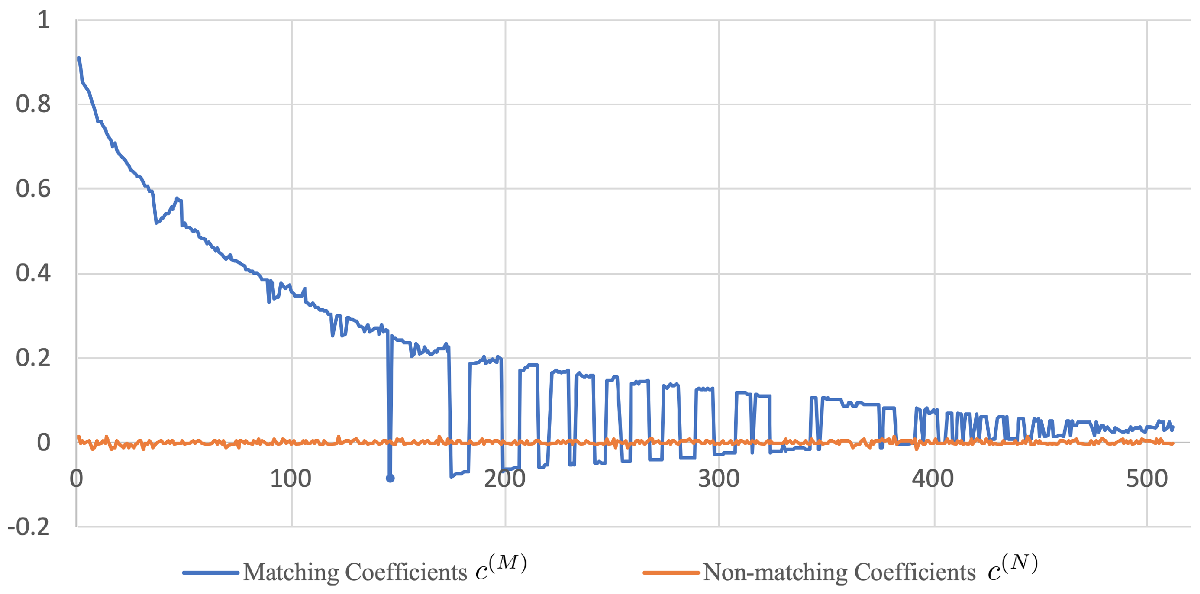
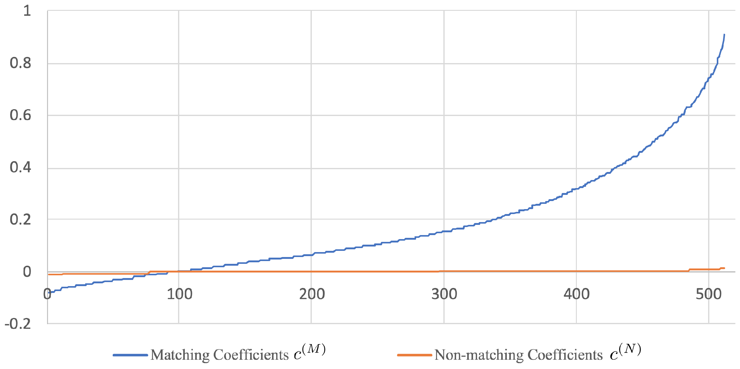
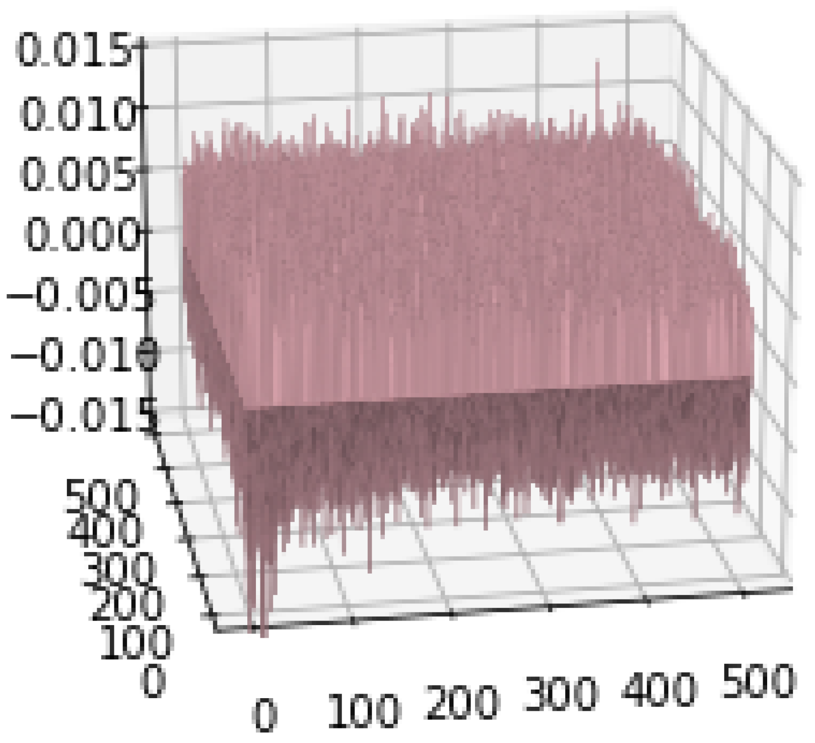
Since is a diagonal matrix, it follows that are mutually independent with for in the case where is a matching pair. We shall further assume that is also a diagonal matrix, which is justified by the fact that in practice is often very close to a zero matrix (see Figure 3 and Figure 4 for some empirical evidences). As a consequence, are mutually independent with for in the case where is a non-matching pair. To check whether the given two images match or not, one can perform a binary hypothesis test regarding the underlying distribution of : vs. .
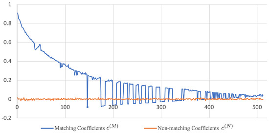
Figure 3.
Profile of the diagonal elements of and (i.e., and , where ) using AVE features. The CCA training was performed on the 120k-SfM dataset.
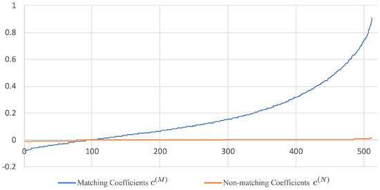
Figure 4.
Profile of sorted diagonal elements of and (i.e., and , where ) using AVE features. The CCA training was performed on the 120k-SfM dataset.
Note that has probability density
while has probability density
We are now in a position to conduct a binary hypothesis test based on the confidence score given below:
3. Experimental Results
3.1. Training Datasets
We resort to two datasets for training, namely, 120k-Structure from Motion (120k-SfM) and 30k-Structure from Motion (30k-SfM) [35]. Both are preprocessed to eliminate overlaps with the evaluation datasets. A succinct description of these two datasets can be found below:
3.1.1. 120k-Structure from Motion
120k-Structure from Motion (120k-SfM) dataset is constructed from the one used in the work of Schonberger et al. [36], which contains 713 3D models with nearly 120k images. The maximum size of each image is . The original dataset includes all image from Oxford5k and Paris6k. Those images are removed to avoid overlaps (in total 98 clusters are eliminated).
3.1.2. 30k-Structure from Motion
30k-Structure from Motion (30k-SfM) dataset is a subset of 120k-SfM, which contains approximately 30k images and 551 classes. The maximum size of images are resized to .
Each dataset serves its own purpose; 30k-SfM is a small dataset while 120k-SfM is a big one. This enables us to investigate the pros and cons of different datasets in terms of their sizes. Compared to 30k-SfM, 120k-SfM supplies richer features to be explored by the methods being tested.
3.2. Training Details
Using each dataset, two lists of matching and non-matching pairs of images are created for training—feature space analysis not CNN training. Table 1 shows some examples of matching and non-matching pairs. Specifically, we randomly select 10,960 raw pairs from 30k-SfM and 58,502 raw pairs from 120k-SfM. We double the number matching and non-matching pairs by simultaneously using each raw pair and its flipped version to ensure that the diagonal/off-diagonal blocks of the data covariances in Equations (1) and (2) are identical and symmetric. This could also be seen from Table 1: each pair is used twice but with its image order flipped.

Table 1.
Examples of matching/non-matching pairs.
The feature vector of a given image is extracted from the very last pooling layer of a pre-trained VGG16 via one of the following three pooling strategies: Global Max (MAC) pooling, Global Average (AVE) pooling, and global Standard Deviation (SD) pooling (global Max (MAC) pooling, Global Average (AVE) pooling, and global Standard Deviation (SD) pooling compute, respectively, the maximum value, the average value, and the standard deviation of the feature map in each channel). We conducted separate training for each of these strategies in order to compare performances.
For benchmarking, the proposed method (G-CCA) and its variant (S-CCA) were trained along with three alternative feature-space analysis methods, i.e., PCAw [21], Supervised PCA (SPCA) [37] and Multiclass LDA (MLDA) [38]. G-CCA is depicted in Figure 2 while S-CCA is the same as G-CCA except that in the final step the scalar similarity measure is used instead (namely, in the last block of Figure 2, is replaced with ). PCAw infers a basis matrix of the feature space from the covariance matrix of the training image features. This basis matrix is used to whiten and compress new image features, which are then leveraged to make a matching/non-matching decision based on the scalar similarity measure. See [12] for a detailed description of the PCAw method and its performance. Furthermore, we compared the proposed method with SPCA, which is a weighted PCA method. It uses a Laplacian matrix to characterize the relationship among the classes in the dataset. We implement SPCA by following the steps in [39]. As to LDA [40], its application to image retrieval has also been thoroughly investigated [41], which is hardly surprising given its popularity in statistical analysis. Here we use its variant MLDA [38] as a competing feature-space analysis method. MLDA is trained using the classes provided by both training datasets. It derives a set of projection vectors that offer the best linear separation of the classes (full separation is achievable if the classes are linearly separable, otherwise, MLDA produces some overlaps between the classes). These projection vectors are employed to transform and compress (in the sense of dimensionality reduction) new feature vectors. Scalar similarity is then evaluated for the transformed features to determine whether or not they match.
3.3. Implementation Details
In the experiment, we compare G-CCA, S-CCA with PCAw, SPCA, and MLDA. The G-CCA and S-CCA are presented in this paper while the PCAw, SPCA, and MLDA are implemented by following procedures in [21,38,39]. Here, we discuss some detailed issues in the implementation.
Firstly, S-CCA, PCAw, SPCA, and MLDA use scalar similarity score to calculate the confidence score while G-CCA uses the proposed score in Equation (8). Secondly, for all these methods, the feature vectors are obtained via MAC, AVE, and SD pooling, and centralization and normalization are performed. Thirdly, the performance comparisons are conducted for eight dimensions: 512, 450, 400, 300, 200, 100, 50, and 25. Lastly, we calculate the scores between the query image and each image in the test dataset, and obtain the image retrieval results by ranking scores from high to low. All the methods are evaluated by the mean Average Precision () (we calculatethe mAP without enforcing the monotonicity for Precision (Recall) relationship). which can be formulated as follows:
where is the average precision for the i-th query image, m is the total number of query images, and n is the total number of images in the testing dataset, is the precision of top k results, and with being the recall of top k results. For calculating the precision and recall , the positive labels for each query image are provided by the test datasets.
3.4. Evaluation Datasets and Details
Four datasets, namely, Oxford5k [42], Paris6k [43], Oxford [44], and Paris [44], are used to assess the performance of each retrieval method. As the first two datasets are contained in the large raw 120k-SfM dataset, they are excluded from the training dataset via preprocessing. The last two datasets contain new annotations and more difficult query images, and consequently create more challenges for image retrieval; therefore, they can help test the reliability of our approach. A short description of each dataset is given below.
3.4.1. Oxford5k
Oxford5k dataset contains 5063 images and 55 query images for 11 different buildings. It is annotated with bounding boxes for the main objects.
3.4.2. Oxford
Oxford dataset contains 4993 images and 70 query images for 11 different buildings. Query images are excluded from the retrieval images. Same as Oxford5k, it is annotated with bounding boxes for the main objects.
3.4.3. Paris6k
Paris6k dataset contains 6412 images and 55 query images for 11 different buildings. It is also annotated with bounding boxes.
3.4.4. Paris
Paris dataset contains 6322 images and 70 query images for 11 different buildings. Query images are excluded from the retrieval images. Same as Paris6k, it is annotated with bounding boxes.
The performance of each retrieval method is evaluated using mean Average Precision (mAP) [42]. The positive labels of each query image are provided by the datasets. The standard evaluation protocol is followed for Oxford5k and Paris6k. As for the Oxford and Paris datasets, the medium protocol setups in [44] are adopted. We crop all the query images with the provided bounding boxes before feeding them to VGG16. Each method undergoes training and evaluation twice. The first training used the small dataset, 30k-SfM, followed by evaluation. Then it was trained with the large dataset, 120k-SfM, before evaluation. This enables us to study the effect of dataset size and diversity on the methods under comparison.
3.5. Performance Evaluation and Analysis
Before getting into the performance evaluation of the proposed method, it is useful to have some insights about how discriminative the canonical vectors are. Figure 5 and Figure 6 show the profile of the diagonal elements of the off-diagonal blocks in Equations (3) and (4). It can be seen that the values of fluctuate around zero whereas those of range between and . This observation suggests that there exists a set of canonical vectors that can effectively tell apart matching from non-matching pairs of images. This is shown in the rest of this subsection.
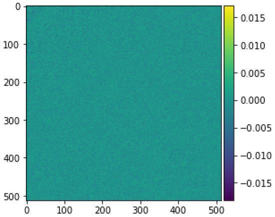
Figure 5.
A 2D visualization of matrix .

Figure 6.
A 3D visualization of matrix .
Table 2 reports the baseline performances of MAC, AVE, and SD without dimensionality reduction. Specifically, for these baselines, we directly calculate the scalar similarity between the pooling features (after centralization and normalization) of the query image and each image in the testing dataset. In the evaluation, we consider the proposed method (G-CCA) and its variant with Gaussian-distribution-based hypothesis testing replaced by scalar similarity (S-CCA). From Table 2, we observe that G-CCA achieves better performance than S-CCA in most cases except for Paris6k and AVE on Paris.
Table 2.
Performance comparison of the baseline, S-CCA, and G-CCA on Oxford5k, Oxford, Paris6k, and Paris without dimension reduction.
By considering three different pooling strategies, three image retrieval methods are trained on the 30k-SfM dataset and evaluated on all four test sets. Table 3 provides a comprehensive depiction of the experimental results for each retrieval method with different pooling strategies and feature dimensionality choices (compression levels). The results for MLDA are not reported there, for MLDA cannot be trained on the 30k-SfM dataset, which is a consequence of the fact that the difference between classes is too small as far as MLDA training is concerned. From Table 3, four observations can be made. The first is regarding the effect of the pooling strategy. Specifically, SD pooling appears to result in the most competitive performance for all methods at every choice of feature dimensionality while MAC renders G-CCA superior to SPCA and PCAw at low dimensions over all test sets. The second observation is that for MAC, AVE, and SD pooling strategies, the proposed method outperforms PCAw at low feature dimensionality. As such, the proposed method is a better choice for producing compact features than PCAw regardless of the pooling strategy. The last observation is that G-CCA is more robust against dimensionality reduction than S-CCA.
Table 3.
Evaluation results from 30k-SfM on Oxford5k, Oxford, Paris6k, and Paris.
The performance of the proposed method can be improved by replacing 30k-SfM with 120k-SfM, which is a larger training set. Table 4 shows the corresponding evaluation results for all the methods with different pooling strategies and dimensionality choices (the only exception is SPCA for which the training on 120k-SfM is computationally infeasible as its Laplacian matrix is too large to be stored on our computer). It is clear that the increased-size training set leads to an improved mAP performance on all test sets and for all pooling strategies. It is also interesting to note that the proposed method outperforms all others on Oxford5k. This uniform superiority across all dimensions is only attained on Paris6k using SD pooling. Although AVE and MAC improve mAP, they cause G-CCA to lose its edge at high dimensions on Paris6k. In contrast, with SD pooling, the proposed method retains its dominating performance at all feature dimensions. On Oxford and Paris, the performance of G-CCA is better than MLDA at almost all dimensions with MAC. G-CCA almost outperforms PCAw in every dimensions with all three pooling strategies.
Table 4.
Evaluation results from 120k-SfM on Oxford5k, Oxford, Paris6k, and Paris.
Based on Table 3 and Table 4, there are three notable advantages of G-CCA over MLDA, PCAw, and SPCA. The first is that the CCA-based methods can be trained using datasets with small differences between classes whereas MLDA cannot be trained on such datasets. The second advantage is that G-CCA typically shows a more graceful performance degradation than PCAw after dimensionality reduction. The last is that SPCA can not be trained on large datasets as compared with G-CCA.
Table 5, Table 6 and Table 7 present some retrieval results for visual illustration. In Table 5, a query image from the Oxford5k set is presented to PCAw, SPCA, and G-CCA, trained on the 30k-SfM set, while in Table 6 and Table 7, a query image from the Oxford5k set is presented to PCAw, MLDA, and G-CCA, trained on the 120k-SfM set. We list top 10 matches for each method with each list ranked using the matching score associated with the corresponding method. Table 5 and Table 6 show the top 10 retrieved images for different methods with SD pooling while Table 7 gives examples for G-CCA with different pooling strategies.
Table 5.
Image retrieval comparison of PCAw, SPCA, and G-CCA.
Table 6.
Image retrieval comparison of PCAw, MLDA, and G-CCA.
Table 7.
Image retrieval comparison of G-CCA with MAC, AVE, and SD feature.
4. Conclusions
In view of the success of DL in image classification, a CCA-based method is proposed to exploit DL features for image retrieval applications. By adopting an OTS CNN without fine-tuning, it achieves good retrieval accuracy with a minimal computational overhead. As shown by the experimental results on standard evaluation datasets, the proposed method is performance-wise competitive against traditional and other OTS-CNN-based methods. Moreover, it exhibits improved robustness against dimensionality reduction and enhanced sensitivity to feature mismatch.
Author Contributions
Data curation, K.S.; Methodology, J.L. and J.C.; Software, K.S., X.L., M.A., X.G. and H.L.; Supervision, J.C.; Writing–original draft, K.S.; Writing–review and editing, M.A., J.C. All authors have read and agreed to the published version of the manuscript.
Funding
This research was supported in part by the Natural Sciences and Engineering Research Council (NSERC) of Canada through a Discovery Grant.
Data Availability Statement
The source code is available at https://github.com/ShiKangdi/Image-Retrieval-via-Canonical-Correlation-Analysis-and-Binary-Hypothesis-Testing.
Conflicts of Interest
The authors declare no conflict of interest.
Appendix A. Chernoff Information between Two 2-Dimensional Gaussian Distributions
For notational simplicity, we suppress subscript t in the following derivation. Consider
where and are two corresponding coefficients. Let , . Now we proceed to find the solution of the equation .
Note that
We have
It can be verified that
where
As a consequence,
Therefore, is a root in of the following quadratic equation:
where
We shall show that Equation (A1) has a unique root in , which is given by
Clearly, Equation (A1) must have a root in since , , and . So it remains to prove the uniqueness of this root.
First consider the case . It is clear that and
where the first inequality is due to . Therefore, the two roots of Equation (A1) must be of different signs, which implies that there exists a unique root in with the expression given by Equation (A2).
Next consider the case . Define . Equation (A1) can be written equivalently as
i.e.,
Note that
and
Therefore, Equation (A3) can be rewritten as
where
A similar argument to that for the case can be used to prove that Equation (A4) has one root in and the other root in . This implies that Equation (A1) must have one root in and the other root in ; the one in must be given by Equation (A2) (note that when ).
References
- Wengang, Z.; Houqiang, L.; Qi, T. Recent advance in content-based image retrieval: A literature survey. arXiv 2017, arXiv:1706.06064. [Google Scholar]
- Lowe, D.G. Distinctive image features from scale-invariant keypoints. Int. J. Comput. Vis. 2004, 60, 91–110. [Google Scholar] [CrossRef]
- Ojala, T.; Pietikainen, M.; Maenpaa, T. Multiresolution gray-scale and rotation invariant texture classification with local binary patterns. IEEE Trans. Pattern Anal. Mach. Intell. 2002, 24, 971–987. [Google Scholar] [CrossRef]
- Tan, X.; Triggs, B. Enhanced local texture feature sets for face recognition under difficult lighting conditions. IEEE Trans. Image Process. 2010, 19, 1635–1650. [Google Scholar] [PubMed] [Green Version]
- Ojansivu, V.; Heikkilä, J. Blur insensitive texture classification using local phase quantization. In International Conference on Image and Signal Processing; Springer: Berlin/Heidelberg, Germany, 2008; pp. 236–243. [Google Scholar]
- Dalal, N.; Triggs, B. Histograms of oriented gradients for human detection. IEEE Conf. Comput. Vis. Pattern Recognit. 2005, 1, 886–893. [Google Scholar]
- Batool, A.; Nisar, M.W.; Shah, J.H.; Khan, M.A.; El-Latif, A.A.A. iELMNet: Integrating novel improved extreme learning machine and convolutional neural network model for traffic sign detection. Big Data, 2022; ahead of print. [Google Scholar] [CrossRef]
- Nawaz, M.; Nazir, T.; Javed, A.; Tariq, U.; Yong, H.-S.; Khan, M.A.; Cha, J. An efficient deep learning approach to automatic glaucoma detection using optic disc and optic cup localization. Sensors 2022, 22, 434. [Google Scholar] [CrossRef]
- Razavian, A.S.; Azizpour, H.; Sullivan, J.; Carlsson, S. CNN features off-the-shelf: An astounding baseline for recognition. In Proceedings of the IEEE Conference on Computer Vision and Pattern Recognition, Columbus, OH, USA, 23–28 June 2014; Institute of Electrical and Electronics Engineers: Columbus, OH, USA, 2014; pp. 806–813. [Google Scholar]
- Khan, M.A.; Muhammad, K.; Sharif, M.; Akram, T.; Kadry, S. Intelligent fusion-assisted skin lesion localization and classification for smart healthcare. Neural Comput. Appl. 2021, 1–16. [Google Scholar] [CrossRef]
- Tolias, G.; Sicre, R.; Jégou, H. Particular object retrieval with integral max-pooling of CNN activations. arXiv 2015, arXiv:1511.05879. [Google Scholar]
- Babenko, A.; Lempitsky, V. Aggregating local deep features for image retrieval. In Proceedings of the IEEE International Conference on Computer Vision, Santiago, Chile, 7–13 December 2015; pp. 1269–1277. [Google Scholar]
- Lin, J.; Duan, L.-Y.; Wang, S.; Bai, Y.; Lou, Y.; Chandrasekhar, V.; Huang, T.; Kot, A.; Gao, W. Hnip: Compact deep invariant representations for video matching, localization, and retrieval. IEEE Trans. Multimed. 2017, 19, 1968–1983. [Google Scholar] [CrossRef]
- Kalantidis, Y.; Mellina, C.; Osindero, S. Cross-dimensional weighting for aggregated deep convolutional features. In European Conference on Computer Vision; Springer: Berlin/Heidelberg, Germany, 2016; pp. 685–701. [Google Scholar]
- Azhar, I.; Sharif, M.; Raza, M.; Khan, M.A.; Yong, H.-S. A decision support system for face sketch synthesis using deep learning and artificial intelligence. Sensors 2021, 21, 8178. [Google Scholar] [CrossRef] [PubMed]
- Khan, S.; Khan, M.A.; Alhaisoni, M.; Tariq, U.; Yong, H.-S.; Armghan, A.; Alenezi, F. Human action recognition: A paradigm of best deep learning features selection and serial based extended fusion. Sensors 2021, 21, 7941. [Google Scholar] [CrossRef]
- Noh, H.; Araujo, A.; Sim, J.; Weyand, T.; Han, B. Largescale image retrieval with attentive deep local features. In Proceedings of the IEEE International Conference on Computer Vision, Venice, Italy, 22–29 October 2017; pp. 3456–3465. [Google Scholar]
- Arandjelovic, R.; Gronat, P.; Torii, A.; Pajdla, T.; Sivic, J. NetVLAD: CNN architecture for weakly supervised place recognition. In Proceedings of the IEEE Conference on Computer Vision and Pattern Recognition, Las Vegas, NV, USA, 26–30 June 2016; pp. 5297–5307. [Google Scholar]
- Radenović, F.; Tolias, G.; Chum, O. CNN image retrieval learns from bow: Unsupervised fine-tuning with hard examples. In European Conference on Computer Vision; Springer: Berlin/Heidelberg, Germany, 2016; pp. 3–20. [Google Scholar]
- Gordo, A.; Almazan, J.; Revaud, J.; Larlus, D. End-to-end learning of deep visual representations for image retrieval. Int. J. Comput. Vis. 2017, 124, 237–254. [Google Scholar] [CrossRef] [Green Version]
- Hyvärinen, A.; Hurri, J.; Hoyer, P.O. Principal components and whitening. In Natural Image Statistics; Springer: Berlin/Heidelberg, Germany, 2009; pp. 93–130. [Google Scholar]
- Izenman, A.J. Linear discriminant analysis. In Modern Multivariate Statistical Techniques; Springer: Berlin/Heidelberg, Germany, 2013; pp. 237–280. [Google Scholar]
- Johnson, R.A.; Wichern, D.W. Canonical correlation analysis. In Applied Multivariate Statistical Analysis, 6th ed.; Pearson: Upper Saddle River, NJ, USA, 2018; pp. 539–574. [Google Scholar]
- Gong, Y.; Ke, Q.; Isard, M.; Lazebnik, S. A multi-view embedding space for modeling internet images, tags, and their semantics. Int. J. Comput. Vis. 2014, 106, 210–233. [Google Scholar] [CrossRef] [Green Version]
- Yan, F.; Mikolajczyk, K. Deep correlation for matching images and text. In Proceedings of the Conference on Computer Vision and Pattern Recognition, Boston, MA, USA, 7–12 June 2015; pp. 3441–3450. [Google Scholar]
- Dorfer, M.; Schlüter, J.; Vall, A.; Korzeniowski, F.; Widmer, G. End-to-end cross-modality retrieval with cca projections and pairwise ranking loss. Int. J. Multimed. Inf. Retr. 2018, 7, 117–128. [Google Scholar] [CrossRef] [Green Version]
- Yu, Y.; Tang, S.; Aizawa, K.; Aizawa, A. Category-based deep cca for fine-grained venue discovery from multimodal data. arXiv 2018, arXiv:1805.02997. [Google Scholar] [CrossRef] [PubMed] [Green Version]
- Lin, Z.; Peltonen, J. An information retrieval approach for finding dependent subspaces of multiple views. In International Conference on Machine Learning and Data Mining in Pattern Recognition; Springer: Berlin/Heidelberg, Germany, 2017; pp. 1–16. [Google Scholar]
- Yair, O.; Talmon, R. Local canonical correlation analysis for nonlinear common variables discovery. IEEE Trans. Signal Process. 2017, 65, 1101–1115. [Google Scholar] [CrossRef]
- Simonyan, K.; Zisserman, A. Very deep convolutional networks for large-scale image recognition. arXiv 2014, arXiv:1409.1556. [Google Scholar]
- Abdi, H. The eigen-decomposition: Eigenvalues and eigenvectors. In Encyclopedia of Measurement and Statistics; SAGE Publications, Inc.: Thousand Oaks, CA, USA, 2007; pp. 304–308. [Google Scholar]
- Nielsen, F. An information-geometric characterization of chernoff information. IEEE Signal Process. Lett. 2013, 20, 269–272. [Google Scholar] [CrossRef] [Green Version]
- Nielsen, F. Chernoff information of exponential families. arXiv 2011, arXiv:1102.2684. [Google Scholar]
- Prince, S.J. Common probability distribution. In Computer Vision: Models, Learning and Inference; Cambridge University Press: Cambridge, England, 2012; pp. 35–42. [Google Scholar]
- Radenović, F.; Tolias, G.; Chum, O. Fine-tuning CNN image retrieval with no human annotation. In IEEE Transactions on Pattern Analysis and Machine Intelligence; Institute of Electrical and Electronics Engineers: Manhattan, NY, USA, 2018. [Google Scholar]
- Schonberger, J.L.; Radenovic, F.; Chum, O.; Frahm, J.-M. From single image query to detailed 3d reconstruction. In Proceedings of the IEEE Conference on Computer Vision and Pattern Recognition, Boston, MA, USA, 7–12 June 2015; pp. 5126–5134. [Google Scholar]
- Koren, Y.; Carmel, L. Robust linear dimensionality reduction. IEEE Trans. Vis. Comput. Graph. 2004, 10, 459–470. [Google Scholar] [CrossRef] [PubMed]
- Li, T.; Zhu, S.; Ogihara, M. Using discriminant analysis for multi-class classification. In Third IEEE International Conference on Data Mining; IEEE Computer Society: Los Alamitos, CA, USA, 2003; p. 589. [Google Scholar]
- Mirkes, E.M.; Gorban, A.N.; Zinoviev, A. A Supervised PCA. 2016. Available online: https://github.com/Mirkes/SupervisedPCA (accessed on 10 September 2021).
- Fisher, R.A. The use of multiple measurements in taxonomic problems. Ann. Eugen. 1936, 7, 179–188. [Google Scholar] [CrossRef]
- Swets, D.L.; Weng, J.J. Using discriminant eigenfeatures for image retrieval. IEEE Trans. Pattern Anal. Mach. Intell. 1996, 8, 831–836. [Google Scholar] [CrossRef] [Green Version]
- Philbin, J.; Chum, O.; Isard, M.; Sivic, J.; Zisserman, A. Object retrieval with large vocabularies and fast spatial matching. In Proceedings of the IEEE Conference on Computer Vision and Pattern Recognition, Minneapolis, MN, USA, 17–22 June 2007; pp. 1–8. [Google Scholar]
- Philbin, J.; Chum, O.; Isard, M.; Sivic, J.; Zisserman, A. Lost in quantization: Improving particular object retrieval in large scale image databases. In Proceedings of the IEEE Conference on Computer Vision and Pattern Recognition, Anchorage, AK, USA, 23–28 June 2008. [Google Scholar]
- Radenovic, F.; Iscen, A.; Tolias, G.; Avrithis, Y.; Chum, O. Revisiting oxford and paris: Large-scale image retrieval benchmarking. In Proceedings of the IEEE Computer Vision and Pattern Recognition Conference, Salt Lake City, UT, USA, 18–23 June 2018. [Google Scholar]


Publisher’s Note: MDPI stays neutral with regard to jurisdictional claims in published maps and institutional affiliations. |
© 2022 by the authors. Licensee MDPI, Basel, Switzerland. This article is an open access article distributed under the terms and conditions of the Creative Commons Attribution (CC BY) license (https://creativecommons.org/licenses/by/4.0/).