DEGAIN: Generative-Adversarial-Network-Based Missing Data Imputation

Abstract

Insights and analysis are only as good as the available data. Data cleaning is one of the most important steps to create quality data decision making. Machine learning (ML) helps deal with data quickly, and to create error-free or limited-error datasets. One of the quality standards for cleaning the data includes handling the missing data, also known as data imputation. This research focuses on the use of machine learning methods to deal with missing data. In particular, we propose a generative adversarial network (GAN) based model called DEGAIN to estimate the missing values in the dataset. We evaluate the performance of the presented method and compare the results with some of the existing methods on publicly available Letter Recognition and SPAM datasets. The Letter dataset consists of 20,000 samples and 16 input features and the SPAM dataset consists of 4601 samples and 57 input features. The results show that the proposed DEGAIN outperforms the existing ones in terms of root mean square error and Frechet inception distance metrics.

1. Introduction

Data cleaning is the process of fixing or removing incorrect, corrupted, incorrectly formatted, duplicate, or incomplete data within a dataset. There are many factors for data to be duplicated or mislabeled, especially when multiple data sources are combined. If data are incorrect, outcomes and algorithms are unreliable, or even the results are incorrect. The exact steps in the data cleaning process is highly dependent on the dataset; however, it is possible to establish a generalized conceptual data cleaning process [1,2] as described in the following:

• Removing duplicate or irrelevant data: When datasets from multiple sources, clients, etc., are combined, the chance of duplicate data creation increases. Additionally, in some analyses, the irrelevant data could also be removed. Any information that does not pertain to the issue that we are attempting to solve is considered irrelevant.
• Fixing structural errors: Structural errors occur when conventions, typos, or incorrect capitalization is observed due to the measurement or data transfer. For instance, if “N/A” and “Not Applicable” both appear, they should be analyzed as the same category.
• Filtering unwanted outliers: If an outlier proves to be irrelevant for analysis or is a mistake, it needs to be removed. Some outliers represent natural variations in the population, and they should be left as is.
• Handling missing data: Many data analytic algorithms cannot accept missing values. There are a few methods to deal with missing data. In general, missing data rows are removed or the missing values are estimated according to the existing data in the dataset. These methods are also known as data imputation.
• Data validation and quality assurance: After completing the previous steps, it is needed to validate the data and to make sure that the data have sufficient quality for the considered analytics.

In this paper, we study the algorithms that are capable of handling the missing data as an important step of data cleaning. Different reasons can lead to missing values during the data collection phase, including, but not limited to, the faulty clinical data registration of patients [3], and sensor damages [4]. One basic method to handle this problem is to remove incomplete data. However, removing the data can diminish the number of samples when the dataset contains many samples with missing values [5]. Therefore, many researchers have tried to employ efficient and effective algorithms to handle the missing values. The effect of the missing data handling methods mainly depends on the missing mechanism. The missing data are categorized as follows [6]:

• Missing completely at random (MCAR): It means that the probability of missing data does not depend on any value of attributes.
• Missing at random (MAR): Meaning that the probability of missing data does not depend on its own particular value, but on the values of other attributes.
• Not missing at random (NMAR): Meaning that the missing data depend on the missed values.

In general, the missing data handling methods could be categorized as data deletion, statistical methods, and machine learning (ML) based approaches. Among the ML based algorithms, generative adversarial networks (GANs) have attracted many researchers in recent years. The GAN has many applications, mostly with a focus on generating synthetic data. The missing value estimation could be considered synthetic data generation. Therefore, it is possible to use such networks in handling the missing data problem. However, the performance of the algorithms is dependent on many variables, such as data type, for instance, if the data belong to the category of an image, clinical dataset, energy dataset, etc. Accordingly, many variations of the GAN are introduced in the literature.

In this study, we conduct a literature review on missing data handling. We present the fundamentals of GAIN [7], a GAN-based algorithm and propose an improved version of GAIN called DEGAIN. In our method, we improve the GAIN by applying the idea of network deconvolution [8]. Convolutional kernels usually re-learn redundant data because of the strong correlations in many image-based datasets. The deconvolution strategy is proven to be effective on images; however, it has not been applied to the GAIN algorithm. DEGAIN is capable of removing the data correlations. We evaluate the performance of the proposed DEGAIN with the publicly available Letter Recognition dataset (Letter dataset, for short) and SPAM dataset. In particular, we use root mean square error (RMSE) and Frechet inception distance (FID) metrics and compare the performance of the proposed DEGAIN with the GAIN, the auto-encoder [9] and the MICE [10] algorithms.

The remainder of this paper is organized as follows: In Section 2, we shortly review the related works. In Section 3, we introduce the system model with mathematical relations and describe the proposed DEGAIN algorithm. The performance evaluation is presented in Section 4. Finally, Section 5 concludes the paper.

2. Related Works

In this section we start with a brief overview of incomplete information management perspectives. Next, we focus our attention on the techniques that replace missing values with the concrete ones and provide a brief review of the existing literature on the missing data handling problem.

2.1. Incomplete Information

Incomplete information arises naturally in many database applications, such as data integration, data exchange, inconsistency management, data cleaning, ontological reasoning, and many others [11].

In some applications, it is natural to allow the presence of incomplete data in the database and to support this circumstance using the proper approaches. The use of null values is the commonly accepted approach for handling incomplete data, and the databases containing null values are usually called incomplete database. Some recent proposals in this direction can be found in [11,12,13,14,15,16].

Intuitively, whenever the database has a structure defined a priori (as in the case of relational databases), some data (for instance, a fax number for a person) to be inserted could be missing. This situation occurs according to the following situations:

• We are sure that the value exists but it is unknown for us;
• We are sure that this value does not exist;
• We do not know anything.

In the relational databases, the unique value, Null, is used in all three situation described before. However, in different applications null values are interpreted as unknown values. In cases like this, we will consider the null values as missing values.

The recent study of [17] that analyzed the use of null values in widely used relational database management systems evidenced that null values are ubiquitous and relevant in real-life scenarios; however, the SQL features designed to deal with them cause multiple problems. While most users accept the SQL behavior for simple queries (positive fragments of relational algebra), many are dissatisfied with SQL answers for more complex queries involving aggregation or negation.

For instance, in some circumscriptions, SQL can miss some tuples that should be considered answers (false negatives); in other cases, SQL can return some tuples that should not be considered answers (false positives). The first situation can be considered an under-approximation of the results and is acceptable in different scenarios. The second one is more critical, as the result might contain incorrect answers. The experimental analysis in [18] showed that false positive are a real problem for queries involving negation. In the observed situations, they were always present and sometimes they constituted almost $100\%$ of the answers.

Theoretical frameworks allow multiple null values in incomplete databases, and the use of labeled nulls provides a more accurate depiction of unknown data. Certain answers, i.e., query answers that can be found from all the complete databases represented by an incomplete database, are a commonly accepted semantics in this paradigm. Unfortunately, the computation of certain answers is a coNP-hard problem [19], which restricts the practical usefulness. A possible solution is to use polynomial time evaluation algorithms computing a sound but possibly an incomplete set of certain answers [11,18,20]. The corresponding prototypes are described in [21,22].

In different applications, missing values cannot be tolerated and must be replaced by the concrete values. It should be noted that in some research works, the authors use the missing data as a feature for other decision makings such as error estimation. For instance the authors in [23] estimate the physical-layer transmission errors in cable broadband networks by considering the missing values. In one of the recent research studies, the authors proposed a new multiple imputation MB (MimMB) framework for causal feature selection with missing data [24]. However, in this paper, we assume that the missing value needs to be handled for further processing activities. The available strategies for handling missing data can be divided into traditional methods and ML-based algorithms, summarized in Figure 1 and described below.

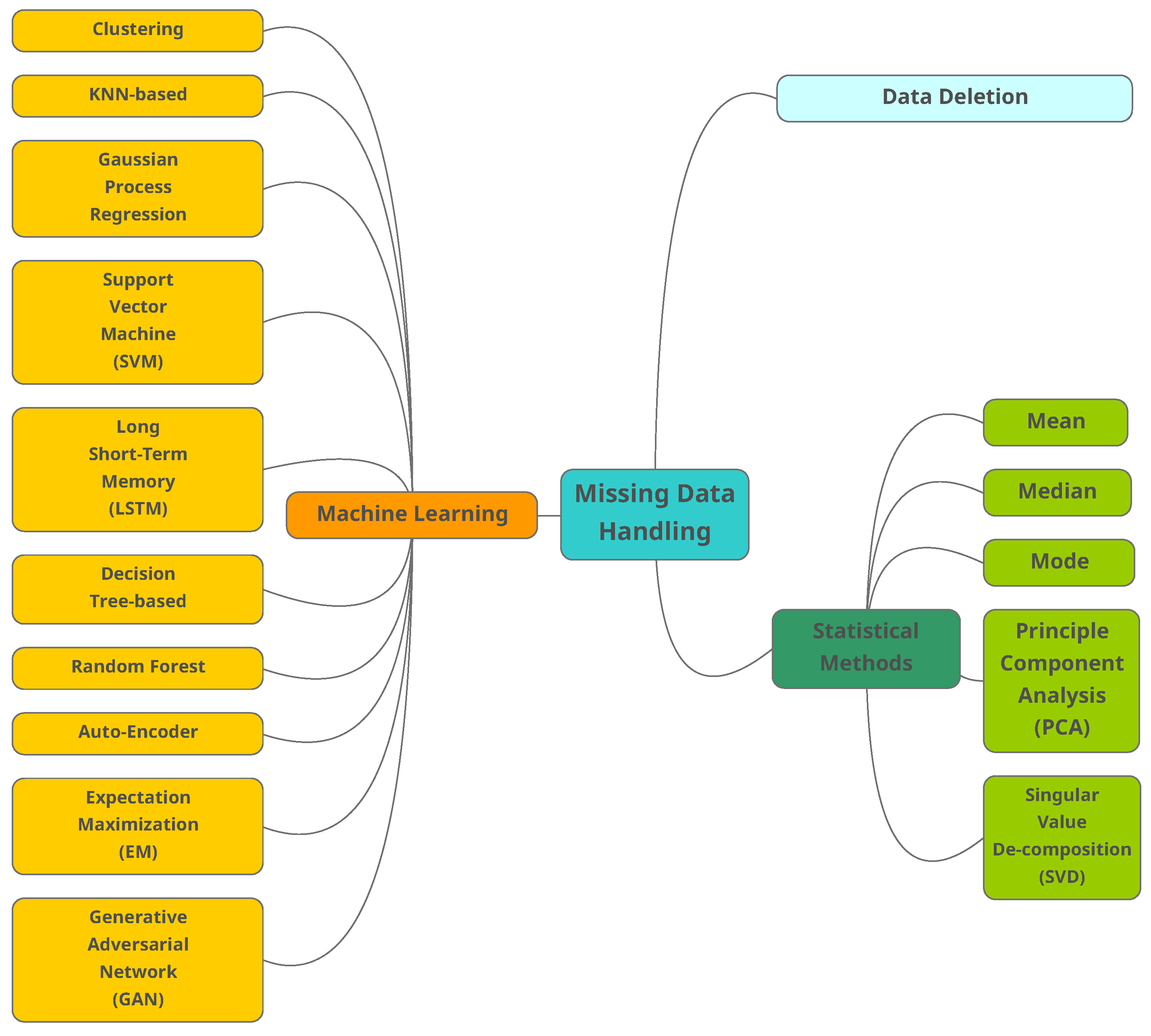
2.2. Traditional Methods

Some of known traditional methods on missing data handling, including the case deletion, mean, median, mode, principal component analysis (PCA) and also singular value decomposition (SVD) are described in the following:

• Case deletion (CD): In CD, missing data instances are omitted. The method has two main disadvantages [25]:
  • Decreasing the dataset size;
  • Since the data are not always MCAR, bias occurs on data distribution and corresponding statistical analysis.
• Mean, median and mode: In these methods, the missing data are replaced with the mean (numeric attribute) of all observed cases. Median is also used to reduce the influence of exceptional data. The characteristic of the original dataset will be changed by using constants to replace missing data, ignoring the relationship among attributes. As an alternative similar solution, we may use the mode of all known values of that attributes to replace the missing data [25]. Mode is usually preferred for categorical data.
• Principal component analysis (PCA): This method is well-known in statistical data analysis and can be used to estimate the data structure level. Traditional PCA cannot deal with the missing data. Upon the measure of variance within the dataset, data will be scored by how well they fit into a principal component (PC). Since the data points will have a PC (the one that best fits), PCA can be considered a clustering analysis. Missing scores are estimated by projecting known scores back into the principal space. More details can be found in [26].
• Singular value decomposition (SVD): In this method, data are projected into another space where the attributes have different values. In the projected space, it is possible to re-construct the missing data.

One of the main differences of the traditional methods and the machine learning based methods to handle the missing data is the capability of the optimization in ML. The ML-based methods follow an optimization process. ML-based methods can also extract the relation between data points, and therefore more precise estimation on the missing values.

2.3. Machine Learning Methods

Machine learning algorithms are categorized into supervised, semi-supervised and unsupervised [27]. Some of the main ML-based methods are clustering algorithms [28], k-nearest neighbors (KNN) [29], Gaussian process regression (GPR) [30], support vector machine (SVM) [31], long short-term memory (LSTM) [32], decision trees (DT) [33], random forests (RF) [34], auto-encoder (AE) [35], expectation maximization (EM) [36] and generative adversarial networks (GAN) [7].

• Clustering: These unsupervised learning algorithms group the samples with similar characters. To replace the missing value, the distance between the centroid of clusters with the sample is calculated, and the missing value of chosen cluster is replaced with the obtained value [28]. The minimum distance could be calculated by a variety of distance functions. One common function is $l^2$-norm [37]. The $l^2$-norm calculates the distance of the vector coordinate from the origin of the vector space.
• k-nearest neighbors (KNN): This supervised algorithm replaces the missing value by the mean (or weighted mean) of the k nearest samples. These neighbor samples are identified by calculating the distance of the missing value with the available samples [28]. Currently, many variations of the original KNN have been proposed in the literature, including the SKNN, IKNN, CKNN, and ICKNN. KNN-based algorithms require heavy calculations to find the nearest neighbors [29]. Some of the common distance functions used in KNN are the Euclidean-overlap metric [38], Value Difference Metric [38] and mean Euclidean distance [38].
• Gaussian process regression (GPR): GPR algorithms predict the output’s variance based on non-linear probabilistic techniques. GPR-based algorithms estimate a probabilistic region for the missing values instead of point estimation. The performance of GRP-based algorithms is dependent on the used kernel function. This kernel is chosen according to the data type and the effective algorithms might use a combination of different kernels. Similar to KNN, the GRP-based algorithms also need heavy calculations, which is not the ideal case for large-scale datasets [30].
• Support vector machine (SVM): SVM has applications in both classification and regression. SVM-based algorithms are non-linear and map the input to a high-dimensional feature space. SVM-based algorithms also use different kernels such as GPR [30].
• Long short-term memory (LSTM): LSTM is a deep learning (DL) algorithm. As a subcategory of recurrent neural networks, DL shows improvement for time series compared with conventional ML algorithms. The training phase of the LSTM might be complex due to the vanishing gradient problem [32].
• Decision tree (DT): DT-based algorithms partition the dataset into groups of samples, forming a tree. The missing data are estimated by the samples associated with the same leaves of the tree. Different variations of DT algorithms have been proposed by researchers, including the ID3, C4.5, CRAT, CHAILD and QUEST [39]. DT algorithms do not require prior information on the data distribution [33].
• Random forest (RF): RF consists of multiple DTs in which the average value of the DT estimation is considered the missing value [34].
• Auto-encoder (AE): As a class of unsupervised DL algorithms, AE learns a coded vector from the input space. The AE generally consists of three layers, including the input, hidden, and output. The objective in AE is to map the input layer to the hidden layer and then reconstruct the input samples through the hidden vector. The elements of input attributes can be missed randomly in the training phase. Therefore, it is expected that the vectors in the input space consist of randomly missing vectors, and the output layer has the complete set of vectors. Performing this task, the AE will learn how to complete the missing data. Different versions of AEs have been introduced, such as VAE, DAE, SAE, and SDAE [35].
• Expectation maximization (EM): EM algorithms are capable of obtaining the local maximum likelihood of a statistical model. These models entail latent variables besides the observed data and unknown parameters. These latent variables can be missing values among the data. The EM-based algorithms guarantee that the likelihood will increase. However, the price is slow convergence rate [36].

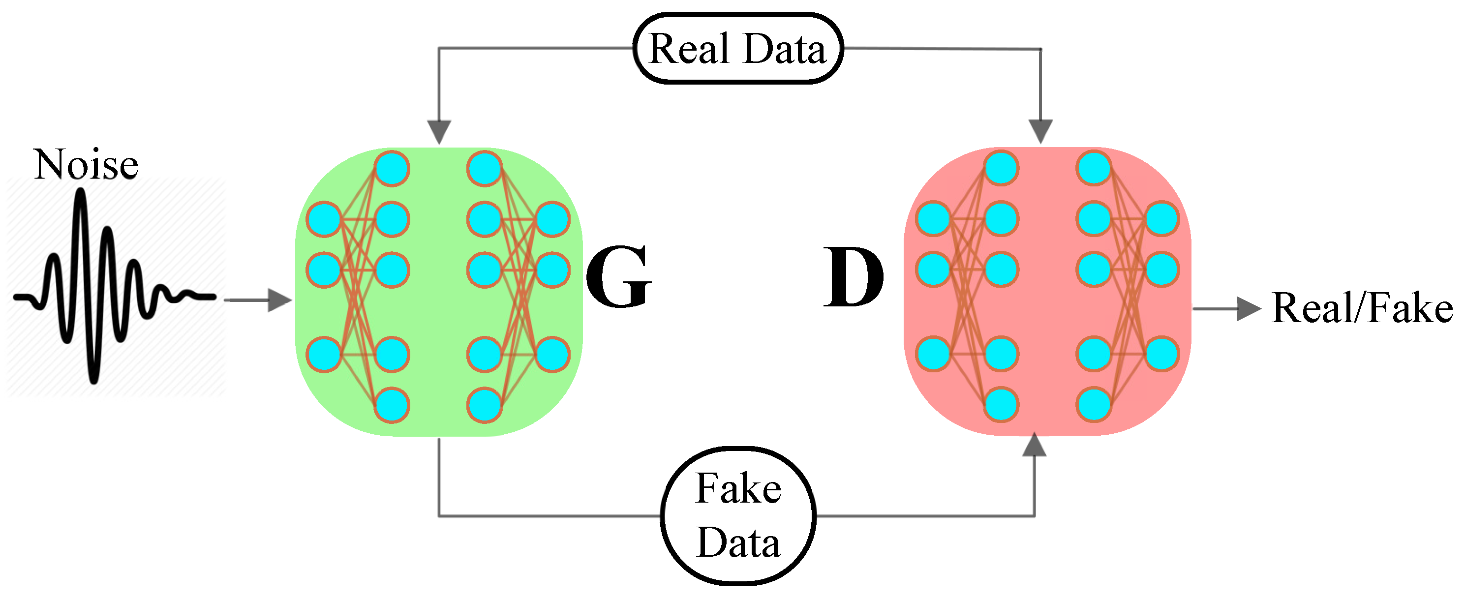
Generative Adversarial Networks

The supervised algorithms need labeled data for the optimization process. However, the data collection for these algorithms is complex. Generative adversarial networks (GANs) can produce synthetic data samples based on a limited set of the collected data. GANs are semi-supervised learning algorithms and generate synthetic data with a small set of collected data. The generated data are not the same as the collected data; however, they are very similar. GANs are among the foremost essential research topic within different research fields, including image-to-image translation, fingerprint localization, classification, speech and language processing, malware detection and video generation [27].

In this section, we introduce the main structure of the GAN, firstly proposed by Goodfellow et al. in 2014 [7]. The GAN consists of two components, the generator (G) and the discriminator (D) as shown in Figure 2. In the training phase, the noise and real data are the input and output of the G component. The dominant goal of the G is to alter the noise to the realistic data. The D component learns to discriminate the real and generated data.

The training process of these two components are based on the pre-defined cost function as presented in Equation (1).

$$\underset{G}{min}\underset{D}{max}L(D,G)=E_{x\sim p_r\left(x\right)}\left[logD\left(\mathbf{x}\right)\right]+E_{z\sim p_z\left(z\right)}\left[log(1-D(G\left(\mathbf{z}\right))\right]$$

(1)

The G and D are two functions and can be denoted by a multi-layer perceptron (MLP). The G learns to alter the noise $\mathbf{z}\sim p_z\left(z\right)$ to the real data. It can be represented by $G(\mathbf{z};{\theta }_g)$ as a function, whose inputs are noise and outputs are generated synthetic data, in which ${\theta }_g$ indicates the parameters of the G component. The D component learns to discern the real and fake data. This component can be represented by $D(\mathbf{x};{\theta }_d)$, whose inputs are real and synthetic data and outputs are class labels, in which ${\theta }_d$ indicates the parameters of the D component. The cost function of the D and G components are presented in Equations (2) and (3), respectively:

$$L\left({\theta }_d\right)=E_{x\sim p_r\left(x\right)}\left[logD(\mathbf{x};{\theta }_d)\right]+E_{z\sim p_z\left(z\right)}\left[log(1-D\left(G(\mathbf{z};{\theta }_g)\right)\right]$$

(2)

$$L\left({\theta }_g\right)=E_{z\sim p_z\left(z\right)}\left[log(1-D\left(G(\mathbf{z};{\theta }_g)\right)\right]$$

(3)

where (${\theta }_d$ and ${\theta }_g$) are updated until convergence is reached. When the real and synthetic data cannot be recognized by the D, the system has reached convergence. Mathematically specking, the convergence occurs when $D(\mathbf{x};{\theta }_d)=0.5$. After the training phase, the G is ready to be utilized for producing the synthetic samples.

3. Proposed Method

3.1. System Model

A GAN-based data imputing method, called generative adversarial imputation nets (GAIN), was introduced in [7]. In GAIN, the generator component G takes real data vectors, imputes the missing values conditioned on the really observed data, and gives a completed vector. Then, the discriminator component D obtains a completed vector and tries to determine which element is really observed and which one is synthesized. To learn the desired distribution in the G component, some additional information is deployed for the discriminator D in the form of a hint vector. The hint vector shows the pieces of information about the missing quality of the real data to the D component, and D concentrates its heed on the quality of imputation for particular missing values. In other words, the hint vector assures the G component to be learned for generating data based on the actual data distribution [7].

Convolution, which applies a kernel to overlapping sections shifted across the data, is a crucial operation in many convolutional neural networks. Although utilizing CNN to synthesize images is not required in GANs, it is frequently done in order to learn the distribution of images [40]. The generator architecture is typically composed of the following layers:

• Linear layer: The noise vector is fed into a fully connected layer, and its output is reshaped into a tensor.
• Batch normalization layer: Stabilizes learning by normalizing inputs to zero mean and unit variance, avoiding training issues, such as vanishing or exploding gradients, and allowing the gradient to flow through the network.
• Up sample layer: Instead of using a convolutional transpose layer to up sample, it mentions using upsampling and then applying a simple convolutional layer on top of it. Convolutional transpose is sometimes used instead.
• Convolutional layer: To learn from up-sampled data, the matrix is passed through a convolutional layer with a stride of 1 and the same padding as it is up sampled.
• ReLU layer: For the generator because it allows the model to quickly saturate and cover the training distribution space.
• TanH Activation: TanH enables the model to converge more quickly.

Convolutional kernels are in fact relearning duplicate data because of the high correlations in real-world data. The convolution makes the neural network training difficult. In the following, we review the mathematical presentation of GAIN.

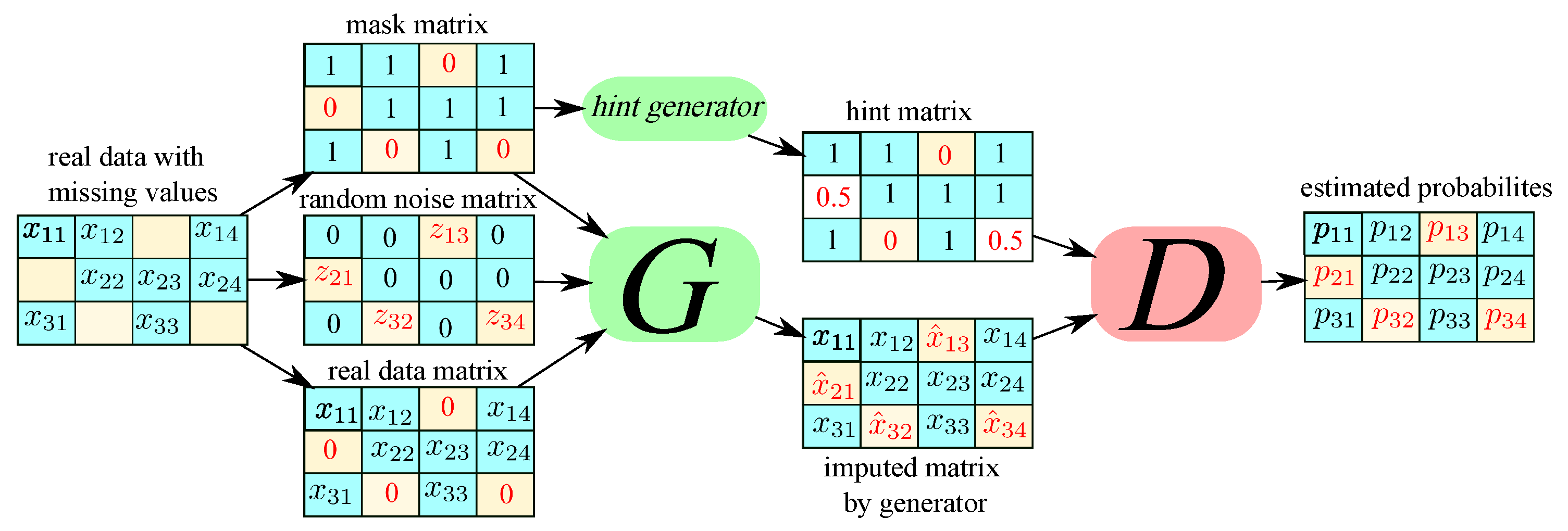
3.2. Problem Formulation

In a d-dimensional space $\mathcal{X}={\mathcal{X}}_1\times \cdots \times {\mathcal{X}}_d$ the $\mathbf{X}=(X_1,\dots ,X_d)$ is a random variable taking values in $\mathcal{X}$ with distribution $P\left(\mathbf{X}\right)$. $\mathbf{M}=(M_1,\dots ,M_d)$ is a random variable in ${\{0,1\}}^d$. The $\mathbf{X}$ is called the data vector, and $\mathbf{M}$ is called the mask vector.

A new space $\widetilde{{\mathcal{X}}_i}={\mathcal{X}}_i\cup \{\ast \}$ is defined for $i\in \{1,\dots ,d\}$ where the start, ∗ does not belong to any ${\mathcal{X}}_i$, and represents an unobserved value. Defining $\tilde{\mathcal{X}}={\tilde{\mathcal{X}}}_1\times \cdots \times {\tilde{\mathcal{X}}}_d$ The variable $\tilde{\mathbf{X}}=({\tilde{X}}_1,\dots ,{\tilde{X}}_d)\in \tilde{\mathcal{X}}$ is presented in Equation (4):

$${\tilde{X}}_i=\left\{\begin{array}{cc}{X}_i,\hfill & \mathrm{if}{M}_i=1\hfill \\ ,\hfill & \mathrm{otherwise}\hfill \end{array}\right.$$

(4)

where $\mathbf{M}$ indicates which components of $\mathbf{X}$ are observed. The $\mathbf{M}$ could be recovered from $\tilde{\mathbf{X}}$. In missing data re-construction, n independent and identically distributed copies of $\tilde{\mathbf{X}}$ are realized, denoted by ${\tilde{\mathbf{x}}}^1,\dots ,{\tilde{\mathbf{x}}}^n$ and defined in the dataset $\mathcal{D}={\left\{({\tilde{\mathbf{x}}}^i,{\mathbf{m}}^i)\right\}}_{i=1}^n$, where ${\mathbf{m}}^i$ is simply the recovered realization of $\mathbf{M}$ corresponding to ${\tilde{\mathbf{x}}}^i$. The goal is to estimate the unobserved values in each ${\tilde{\mathbf{x}}}_i$. The samples are generated according to $P\left(\mathbf{X}\right|\tilde{\mathbf{X}}={\tilde{\mathbf{x}}}^i)$, that is, the conditional distribution of $\mathbf{X}$ given $\tilde{\mathbf{X}}={\tilde{\mathbf{x}}}^i$ for each i to fill in the missing data points in $\mathcal{D}$.

The generator, G, takes as input $\tilde{\mathbf{X}}$, $\mathbf{M}$ and a noise variable $\mathbf{Z}$, and outputs $\overline{\mathbf{X}}$, where $\overline{\mathbf{X}}$ is a vector of synthetic data. Let $G:\tilde{\mathcal{X}}\times {\{0,1\}}^d\times {[0,1]}^d\to \mathcal{X}$ be a function, and $\mathbf{Z}=(Z_1,\dots ,Z_d)$ be d-dimensional noise (independent of all other variables) [7]. The random variables $\overline{\mathbf{X}},\widehat{\mathbf{X}}\in \mathcal{X}$ are defined by Equations (5) and ().

$$\begin{array}{cc}\hfill \overline{\mathbf{X}}& =G(\tilde{\mathbf{X}},\mathbf{M},(\mathbf{1}-\mathbf{M})\odot \mathbf{Z})\hfill \end{array}$$

(5)

$$\begin{array}{cc}\hfill \widehat{\mathbf{X}}& =\mathbf{M}\odot \tilde{\mathbf{X}}+(\mathbf{1}-\mathbf{M})\odot \overline{\mathbf{X}}\hfill \end{array}$$

(6)

where ⊙ denotes element-wise multiplication. $\overline{\mathbf{X}}$ corresponds to the vector of estimated values and $\widehat{\mathbf{X}}$ corresponds to the completed data vector.

The discriminator, D will be used to train G. However, unlike the standard GAN where the output of the generator is either real or synthetic, the output of GAIN is comprised of some components that are real and some that are synthetic. Rather than identifying that an entire vector is real or synthetic, the discriminator attempts to distinguish which are real (observed) or synthetic. The mask vector $\mathbf{M}$ is pre-determined by the dataset. Formally, the discriminator is a function $D:\mathcal{X}\to {[0,1]}^d$ with the i-th component of $D\left(\widehat{\mathbf{x}}\right)$ corresponding to the probability that the i-th component of $\widehat{\mathbf{x}}$ was observed. The D is trained to maximize the probability of correctly predicting $\mathbf{M}$ and G is trained to minimize the probability of D predicting $\mathbf{M}$. The quantity $V(D,G)$ is defined as presented in Equation (7).

$$\begin{array}{cc}\hfill V(D,G)& ={\mathbb{E}}_{\widehat{\mathbf{X}},\mathbf{M},\mathbf{H}}\left[{\mathbf{M}}^{T}logD(\widehat{\mathbf{X}},\mathbf{H})+{(\mathbf{1}-\mathbf{M})}^{T}log\left(\mathbf{1}-D(\widehat{\mathbf{X}},\mathbf{H})\right)\right],\hfill \end{array}$$

(7)

where log is an element-wise logarithm and dependence on G is through $\widehat{\mathbf{X}}$. The goal of GAIN is presented in Equation (8):

$$\underset{G}{min}\underset{D}{max}V(D,G).$$

(8)

where the loss function $\mathcal{L}:{\{0,1\}}^d\times {[0,1]}^d\to \mathbb{R}$ is defined as presented in Equation (9):

$$\mathcal{L}(\mathbf{a},\mathbf{b})=\sum _{i=1}^d\left[a_{i}log\left(b_i\right)+(1-a_i)log(1-b_i)\right].$$

(9)

3.3. Proposed Algorithm: DEGAIN

The proposed DEGAIN is originated from GAIN [7]. The main idea behind the DEGAIN is to use deconvolution in the generator and discriminator. Convolution applies a kernel to overlapping regions shifted across the data. However, because of the strong correlations in real-world data, convolutional kernels are in effect re-learning redundant data. This redundancy makes the neural network training challenging. The deconvolution can remove the correlations before the data are fed into each layer. It has been shown in [8] that the deconvolution can be efficiently calculated at a fraction of the computational cost of a convolution layer. The deconvolution strategy has proven to be effective on images; however, it has not been applied to GANs, including the GAIN.

Given a data matrix $X_{N\times F}$, where N is the number of samples and F is the number of features, the covariance matrix is calculated as $Cov=\frac{1}{N}{(X-\mu )}^T(X-\mu )$.

An approximated inverse square root of the covariance matrix could be calculated as $D=Co{v}^{-\frac{1}{2}}$ multiplied with the centered vectors $(X-\mu )·D$. Accordingly, the correlation effects could be removed. If computed perfectly, the transformed data have the identity matrix as covariance: $D^T{(X-\mu )}^T(X-\mu )D=Co{v}^{-0.5}·Cov·Co{v}^{-0.5}=I$.

The process to construct X and $D\approx {(Cov+ϵ·I)}^{-\frac{1}{2}}$ is presented in Algorithm 1, where $ϵ·I$ improves the stability. The deconvolution operation is further applied via matrix multiplication to remove the correlation between neighboring pixels. The deconvolved data are then multiplied with w. The architecture of proposed method is depicted in Figure 3. When the training phase is completed, the G component is able to impute the dataset. There are two main loops for updating the parameters of the G and D components in Algorithm 1. First, batch samples from the noise and samples of real data are presented to the inner loop for updating the parameters of the D component. The cost function of the D component is then calculated by the given samples. Then, the D component’s parameters are updated based on the initiated rate.

Algorithm 1 (The DEGAIN algorithm: deconvolution and then training).

1: Input: N channels of input features $[x_1,x_2,\dots ,x_N]$, Number of epochs e; Number of Iteration of inner loop n; Updating rates (${\alpha }_g$ and ${\alpha }_d$); 2: for$i\in \{1,\dots ,N\}$do 3:    $X_i=im2col\left(x_i\right)$ 4: $X=[X_1,\dots ,X_N]$ 5: $X=Reshape\left(X\right)$ 6: $Cov=\frac{1}{M}{X}^{t}X$ %$\left[x_i\right]\mathrm{has}M\mathrm{rows}$ 7: $D\approx {(Cov+ϵ·I)}^{-\frac{1}{2}}$ Training of G and D 8: for ($i=0$; $i<e$; i++) do 9:    for $j=0$; $j<n$; j++ do 10:        batch samples from noise $Z\in R^{B\times L}\sim p_z\left(z\right)$; 11:        batch samples from noise $X\in R^{B\times M}$; 12:        $L\left({\theta }_d\right)=\frac{1}{B}{\Sigma }_{b=1}^{B}logD(X_b,{\theta }_d)+log(1-D(G\left(2Z_b\right),{\theta }_g))$; 13:        ${\xi }_d=\frac{\delta }{\delta {\theta }_d}L\left({\theta }_d\right)$; 14:        ${\theta }_d^{j+1}={\theta }_d^t+{\alpha }_d{\xi }_d$ 15:    batch samples from noise $Z\in R^{B\times L}\sim p_z\left(z\right)$; 16:    $L\left({\theta }_d\right)=\frac{1}{B}{\Sigma }_{b=1}^{B}log(1-D\left(G(Z_b,{\theta }_g)\right))$ 17:    ${\xi }_d=\frac{\delta }{\delta {\theta }_d}L\left({\theta }_d\right)$; 18:    ${\theta }_g^{i+1}={\theta }_g^t-{\alpha }_g{\xi }_g$;

4. Performance Evaluation

We evaluate the performance of the DEGAIN and compare the results with MICE [10], GAIN [7] and AE [9]. Multivariate imputation by chained equations (MICE) has emerged in addressing missing data. The chained equations approach can handle variables of varying types, for instance, the continuous or binary as well as complexities such as bounds. MICE is also a software package presented in R [10]. In multiple imputation algorithms such as AE, multiple copies of the dataset are replaced by slightly different imputed values in each copy. In this method, the variability is modeled into the imputed values [9].

We perform each experiment 10 times, and within each experiment, we use 5-cross validations in terms of RMSE, which directly measures the error distance, and FID, which takes the distribution of imputed values into account. We use the Letter and SPAM datasets for comparing algorithms, and samples are missed with the rate of 20%.

4.1. Evaluation Metrics

In our experiments we consider the root-mean-square error (RMSE) and Frechet inception distance (FID) metrics to evaluate the performance of the proposed DEGAIN on handling the missing data. It should be noted that besides RMSE and FID, several other metrics are introduced in the literature including, but not limited to, mean absolute error (MAE), area under ROC curve or AUC score and F1-score. These metrics perform in different datasets or operations. For example, the F1-score is mostly used for binary classification. MAE is similar to RMSE; however, RMSE is more common in the literature. Comparing our method with GAIN, AE and MICE, we chose the related RMSE and FID metrics. Remember that RMSE is used for continuous values and measures the error between real values and imputed values for an incomplete dataset. FID converts a group of imputed samples to a feature space using a particular inception net layer. Assuming the converted layer as a continuous multivariate Gaussian distribution, the mean and covariance are predicted for both the imputed and real samples.

The mathematical presentation is shown in

Table 1. Evaluation metrics used to assess the proposed algorithm’s performance.

Metric	Formula
RMSE	$RMSE=\sqrt{\frac{1}{\widehat{N}}{\displaystyle \sum _{i=1}^{\widehat{N}}}{(y_i-{\widehat{y}}_i)}^2}$
FID	$d^2\left((m_1,C_1)(m_2,C_2)\right)={∥m_1-m_2∥}_2^2+\mathrm{Tr}(C_1+C_2-2{\left(C_1{C}_2\right)}^{\frac{1}{2}})$

, where $\widehat{N}$ is the number of missing values, $y_i$ is the real missing value, and ${\widehat{y}}_i$ is the imputed value. Additionally, the $m_1$ and $m_2$ denote the mean of the real and imputed data, respectively. $C_1$ and $C_2$ indicate the covariance of real and imputed data, respectively.

4.2. Dataset

Here we use the Letter and SPAM datasets. Letter is publicly available in the UC Irvine Machine Learning Repository and can be accessed through https://archive.ics.uci.edu/ (accessed on 20 July 2022). In this dataset, the objective is to identify each of a large number of black-and-white rectangular pixel displays as one of the 26 capital letters in the English alphabet. The character images are based on 20 different fonts and each letter within these 20 fonts is randomly distorted to produce a file of 20,000 unique stimuli. Typically, the first 16,000 items are used for training and then the resulting model is capable of predicting the letter category for the remaining 4000. The SPAM dataset consists of 4601 samples and 57 input features. In this dataset, the goal is to predict spam emails based on input features. SPAM is also publicly available at http://archive.ics.uci.edu/ml/datasets/Spambase/ (accessed on 10 August 2022). These datasets have no missing values and therefore, we use a 20% rate of missed samples.

4.3. Results

The evaluation are performed in Google Colab, on Python 3 with 12 GB of RAM. We used the base codes of GAIN [7] publicly accessible in https://github.com/jsyoon0823/GAIN (accessed on 10 July 2022). We modified the code and added the deconvolution to the Generator and Discriminator. The results are presented in

Table 2. Performance evaluations of proposed DEGAIN, GAIN [7], AE [9], MICE [10] in terms of RMSE and FID metrics.

	Proposed DEGAIN	GAIN [7]	AE [9]	MICE [10]
RMSE (Letter dataset)	0.096	0.101	0.142	0.166
Normalized FID (Letter dataset)	0.492	0.513	0.826	1
RMSE (SPAM dataset)	0.047	0.050	0.064	0.068
Normalized FID (SPAM dataset)	0.898	0.946	0.973	1

and illustrated in Figure 4. As can be seen in Table 2 and Figure 4, the performance of GAN-based algorithms, both GAIN and DEGAIN perform much better than the auto-encoder (AE) [9] and MICE [10]. The DEGAIN is slightly better compared with the GAIN. The main advantage of the DEGAIN could be explored running on correlated large datasets of images. Therefore, as expected, the GAIN and proposed DEGAIN can be the most profitable in image datasets.

5. Conclusions

In this paper, we studied the traditional and machine learning based algorithms that could handle the missing data problem in data cleaning process. We reviewed the architecture of generative adversarial network (GAN) based models and their performance on missing data handling. We proposed an algorithm called DEGAIN to estimate the missing values in the dataset. The DEGAIN is based on the known GAIN algorithm that is already used in missing data imputation. We added deconvolution to remove the correlation between data. The evaluated performance of the presented method was performed on publicly available datasets, called Letter and SPAM. The RMSE and FID metrics on the results confirmed that the GANs are effective on re-constructing the missing values compared with the earlier auto-encoder or MICE algorithms. Additionally, the proposed DEGAIN performed well and improved the performance of GAIN. We believe that the main advantages of DEGAIN could be explored running on large image datasets, although it showed improvement even on our chosen datasets. This paper addresses one of many aspects of data quality: missing information. Inconsistent information, which could be handled using methods such as arbitration [41], is still an open issue that GAN-based methods and the proposed DEGAIN need to address in future works.

References

1. Ilyas, I.F.; Chu, X. Data Cleaning; Morgan & Claypool: San Rafael, CA, USA, 2019. [Google Scholar]
2. O’Brien, A.D.; Stone, D.N. Yes, you can import, analyze, and create dashboards and storyboards in Tableau! The GBI case. J. Emerg. Technol. Account. 2020, 17, 21–31. [Google Scholar] [CrossRef]
3. Luo, Y. Evaluating the state of the art in missing data imputation for clinical data. Briefings Bioinform. 2022, 23, bbab489. [Google Scholar] [CrossRef] [PubMed]
4. Li, Y.; Bao, T.; Chen, H.; Zhang, K.; Shu, X.; Chen, Z.; Hu, Y. A large-scale sensor missing data imputation framework for dams using deep learning and transfer learning strategy. Measurement 2021, 178, 109377. [Google Scholar] [CrossRef]
5. Platias, C.; Petasis, G. A Comparison of Machine Learning Methods for Data Imputation. In Proceedings of the 11th Hellenic Conference on Artificial Intelligence, Athens, Greece, 2–4 September 2020; pp. 150–159. [Google Scholar]
6. Austin, P.C.; White, I.R.; Lee, D.S.; van Buuren, S. Missing data in clinical research: A tutorial on multiple imputation. Can. J. Cardiol. 2021, 37, 1322–1331. [Google Scholar] [CrossRef] [PubMed]
7. Yoon, J.; Jordon, J.; Schaar, M. Gain: Missing data imputation using generative adversarial nets. In Proceedings of the International Conference on Machine Learning, Stockholm, Sweden, 10–15 July 2018; pp. 5689–5698. [Google Scholar]
8. Ye, C.; Evanusa, M.; He, H.; Mitrokhin, A.; Goldstein, T.; Yorke, J.A.; Fermüller, C.; Aloimonos, Y. Network deconvolution. arXiv 2019, arXiv:1905.11926. [Google Scholar]
9. Gondara, L.; Wang, K. Multiple imputation using deep denoising autoencoders. arXiv 2017, arXiv:1705.02737. [Google Scholar]
10. Van Buuren, S.; Groothuis-Oudshoorn, K. mice: Multivariate imputation by chained equations in R. J. Stat. Softw. 2011, 45, 1–67. [Google Scholar] [CrossRef] [Green Version]
11. Greco, S.; Molinaro, C.; Trubitsyna, I. Approximation algorithms for querying incomplete databases. Inf. Syst. 2019, 86, 28–45. [Google Scholar] [CrossRef]
12. Calautti, M.; Console, M.; Pieris, A. Benchmarking approximate consistent query answering. In Proceedings of the 40th ACM SIGMOD-SIGACT-SIGAI Symposium on Principles of Database Systems, Virtual Event, China, 20–25 June 2021; pp. 233–246. [Google Scholar]
13. Calautti, M.; Caroprese, L.; Greco, S.; Molinaro, C.; Trubitsyna, I.; Zumpano, E. Existential active integrity constraints. Expert Syst. Appl. 2021, 168, 114297. [Google Scholar] [CrossRef]
14. Calautti, M.; Greco, S.; Molinaro, C.; Trubitsyna, I. Query answering over inconsistent knowledge bases: A probabilistic approach. Theor. Comput. Sci. 2022, 935, 144–173. [Google Scholar] [CrossRef]
15. Calautti, M.; Greco, S.; Molinaro, C.; Trubitsyna, I. Preference-based Inconsistency-Tolerant Query Answering under Existential Rules. Artif. Intell. 2022, 312, 103772. [Google Scholar] [CrossRef]
16. Calautti, M.; Greco, S.; Molinaro, C.; Trubitsyna, I. Querying Data Exchange Settings Beyond Positive Queries. In Proceedings of the 4th International Workshop on the Resurgence of Datalog in Academia and Industry (Datalog-2.0), Genova, Italy, 5 September 2022; Volume 3203, pp. 27–41. [Google Scholar]
17. Toussaint, E.; Guagliardo, P.; Libkin, L.; Sequeda, J. Troubles with nulls, views from the users. Proc. VIDB Endow. 2022, 15, 2613–2625. [Google Scholar] [CrossRef]
18. Guagliardo, P.; Libkin, L. Making SQL queries correct on incomplete databases: A feasibility study. In Proceedings of the 35th ACM SIGMOD-SIGACT-SIGAI Symposium on Principles of Database Systems, San Francisco, CA, USA, 26 June–1 July 2016; pp. 211–223. [Google Scholar]
19. Abiteboul, S.; Kanellakis, P.C.; Grahne, G. On the Representation and Querying of Sets of Possible Worlds. Theor. Comput. Sci. 1991, 78, 158–187. [Google Scholar] [CrossRef] [Green Version]
20. Libkin, L. SQL’s three-valued logic and certain answers. ACM Trans. Database Syst. (TODS) 2016, 41, 1–28. [Google Scholar] [CrossRef] [Green Version]
21. Fiorentino, N.; Greco, S.; Molinaro, C.; Trubitsyna, I. ACID: A system for computing approximate certain query answers over incomplete databases. In Proceedings of the International Conference on Management of Data (SIGMOD), Houston, TX, USA, 10–15 June 2018; pp. 1685–1688. [Google Scholar]
22. Fiorentino, N.; Molinaro, C.; Trubitsyna, I. Approximate Query Answering over Incomplete Data. In Complex Pattern Mining; Springer: Berlin, Germany, 2020; pp. 213–227. [Google Scholar]
23. Hu, J.; Zhou, Z.; Yang, X. Characterizing Physical-Layer Transmission Errors in Cable Broadband Networks. In Proceedings of the 19th USENIX Symposium on Networked Systems Design and Implementation (NSDI 22), Renton, WA, USA, 4–6 April 2022; USENIX Association: Renton, WA, USA, 2022; pp. 845–859. [Google Scholar]
24. Yu, K.; Yang, Y.; Ding, W. Causal Feature Selection with Missing Data. ACM Trans. Knowl. Discov. Data 2022, 16, 1–24. [Google Scholar] [CrossRef]
25. Peng, L.; Lei, L. A review of missing data treatment methods. Intell. Inf. Manag. Syst. Technol 2005, 1, 412–419. [Google Scholar]
26. Folch-Fortuny, A.; Arteaga, F.; Ferrer, A. PCA model building with missing data: New proposals and a comparative study. Chemom. Intell. Lab. Syst. 2015, 146, 77–88. [Google Scholar] [CrossRef]
27. Mirtaheri, S.L.; Shahbazian, R. Machine Learning: Theory to Applications; CRC Press: Boca Raton, FL, USA, 2022. [Google Scholar]
28. Nagarajan, G.; Babu, L.D. Missing data imputation on biomedical data using deeply learned clustering and L2 regularized regression based on symmetric uncertainty. Artif. Intell. Med. 2022, 123, 102214. [Google Scholar] [CrossRef]
29. Emmanuel, T.; Maupong, T.; Mpoeleng, D.; Semong, T.; Mphago, B.; Tabona, O. A survey on missing data in machine learning. J. Big Data 2021, 8, 1–37. [Google Scholar]
30. Ma, Y.; He, Y.; Wang, L.; Zhang, J. Probabilistic reconstruction for spatiotemporal sensor data integrated with Gaussian process regression. Probabilistic Eng. Mech. 2022, 69, 103264. [Google Scholar] [CrossRef]
31. Camastra, F.; Capone, V.; Ciaramella, A.; Riccio, A.; Staiano, A. Prediction of environmental missing data time series by Support Vector Machine Regression and Correlation Dimension estimation. Environ. Model. Softw. 2022, 150, 105343. [Google Scholar] [CrossRef]
32. Saroj, A.J.; Guin, A.; Hunter, M. Deep LSTM recurrent neural networks for arterial traffic volume data imputation. J. Big Data Anal. Transp. 2021, 3, 95–108. [Google Scholar] [CrossRef]
33. Cenitta, D.; Arjunan, R.V.; Prema, K. Missing data imputation using machine learning algorithm for supervised learning. In Proceedings of the 2021 International Conference on Computer Communication and Informatics (ICCCI), Coimbatore, India, 27–29 January 2021; pp. 1–5. [Google Scholar]
34. Tang, F.; Ishwaran, H. Random forest missing data algorithms. Stat. Anal. Data Mining: Asa Data Sci. J. 2017, 10, 363–377. [Google Scholar] [CrossRef] [PubMed]
35. Ryu, S.; Kim, M.; Kim, H. Denoising autoencoder-based missing value imputation for smart meters. IEEE Access 2020, 8, 40656–40666. [Google Scholar] [CrossRef]
36. Nelwamondo, F.V.; Mohamed, S.; Marwala, T. Missing data: A comparison of neural network and expectation maximization techniques. Curr. Sci. 2007, 93, 1514–1521. [Google Scholar]
37. Eirola, E.; Doquire, G.; Verleysen, M.; Lendasse, A. Distance estimation in numerical data sets with missing values. Inf. Sci. 2013, 240, 115–128. [Google Scholar] [CrossRef] [Green Version]
38. Santos, M.S.; Abreu, P.H.; Wilk, S.; Santos, J. How distance metrics influence missing data imputation with k-nearest neighbours. Pattern Recognit. Lett. 2020, 136, 111–119. [Google Scholar] [CrossRef]
39. Rokach, L.; Maimon, O. Decision trees. In Data Mining and Knowledge Discovery Handbook; Springer: New York, NY, USA, 2005; pp. 165–192. [Google Scholar]
40. Benjdira, B.; Ammar, A.; Koubaa, A.; Ouni, K. Data-efficient domain adaptation for semantic segmentation of aerial imagery using generative adversarial networks. Appl. Sci. 2020, 10, 1092. [Google Scholar] [CrossRef] [Green Version]
41. Revesz, P.Z. On the semantics of arbitration. Int. J. Algebra Comput. 1997, 7, 133–160. [Google Scholar] [CrossRef]
Figure 1. The categorization of traditional and machine learning based algorithms used for missing data handling.
Information 13 00575 g001
Figure 2. The general structure of GAN proposed by Goodfellow.
Information 13 00575 g002
Figure 3. The general structure of DEGAIN.
Information 13 00575 g003
Figure 4. Illustration of evaluation results on RMSE and FID metrics for proposed DEGAIN, GAIN [7], AE [9] and MICE [10] on Letter dataset.
Information 13 00575 g004