Article

Dynamic Regressor/Ensemble Selection for a Multi-Frequency and Multi-Environment Path Loss Prediction

by
Usman Sammani Sani
1,*,
Owais Ahmed Malik
1,2 and
Daphne Teck Ching Lai
1,*
1
School of Digital Science, Universiti Brunei Darussalam, Tungku Link, Gadong BE1410, Brunei
2
Institute of Applied Data Analytics, Universiti Brunei Darussalam, Tungku Link, Gadong BE1410, Brunei
*
Authors to whom correspondence should be addressed.
Information 2022, 13(11), 519; https://doi.org/10.3390/info13110519
Submission received: 24 August 2022 / Revised: 24 September 2022 / Accepted: 29 September 2022 / Published: 31 October 2022
(This article belongs to the Section Information and Communications Technology)

Abstract

:
Wireless network parameters such as transmitting power, antenna height, and cell radius are determined based on predicted path loss. The prediction is carried out using empirical or deterministic models. Deterministic models provide accurate predictions but are slow due to their computational complexity, and they require detailed environmental descriptions. While empirical models are less accurate, Machine Learning (ML) models provide fast predictions with accuracies comparable to that of deterministic models. Most Empirical models are versatile as they are valid for various values of frequencies, antenna heights, and sometimes environments, whereas most ML models are not. Therefore, developing a versatile ML model that will surpass empirical model accuracy entails collecting data from various scenarios with different environments and network parameters and using the data to develop the model. Combining datasets of different sizes could lead to lopsidedness in accuracy such that the model accuracy for a particular scenario is low due to data imbalance. This is because model accuracy varies at certain regions of the dataset and such variations are more intense when the dataset is generated from a fusion of datasets of different sizes. A Dynamic Regressor/Ensemble selection technique is proposed to address this problem. In the proposed method, a regressor/ensemble is selected to predict a sample point based on the sample’s proximity to a cluster assigned to the regressor/ensemble. K Means Clustering was used to form the clusters and the regressors considered are K Nearest Neighbor (KNN), Extreme Learning Trees (ET), Random Forest (RF), Gradient Boosting (GB), and Extreme Gradient Boosting (XGBoost). The ensembles are any combinations of two, three or four of the regressors. The sample points belonging to each cluster were selected from a validation set based on the regressor that made prediction with lowest absolute error per individual sample point. Implementation of the proposed technique resulted in accuracy improvements in a scenario described by a few sample points in the training data. Improvements in accuracy were also observed on datasets in other works compared to the accuracy reported in the works. The study also shows that using features extracted from satellite images to describe the environment was more appropriate than using a categorical clutter height value.

1. Introduction

Most of modern-day information is sent through the wireless channel due to its low cost and ease of installation when compared with the wired channel [1]. However, as signals propagate through the wireless channel, the strength diminishes in free space due to expansion and presence of obstacles, resulting in reflection, refraction, diffraction, and absorption of the signals, and hence, multipath [2,3,4]. The reduction in signal strength is termed path loss and its computation/prediction is important, particularly during network design, maintenance, or interference analysis, as it helps in setting up network parameters such as transmitter/base station antenna height, cell radius, and transmitting power [5,6]. Prediction of path loss is done using either empirical models, deterministic models, or Machine Learning models (ML) [7,8]. Empirical models are mostly used due to their ease of use and availability in Radio Frequency Planning Softwares [9]. However empirical models have lower accuracy than deterministic models. The problem with deterministic models is their high computational complexity, and requirements for detailed environmental description [8,10,11]. ML models rival deterministic models, having a faster prediction, with high accuracy [12]. Machine Learning algorithms such as K Nearest Neighbor (KNN) [13], Multiple Layer Perceptron (MLP) [8], Support Vector Regression (SVR) [14], Generalized Regression Neural Network (GRNN) [15], Radial Basis Function Neural Network (RBFNN) [16], and Random Forest (RF) [17] have been used in developing path loss models. However, such models were developed for specific environments, with fixed frequencies and antenna heights. Such use of machine learning models is at its early stage of adoption for use in path loss prediction and cannot replace empirical models such as the COST 231 Hata model because most empirical models have parameter ranges in which they are valid in terms of frequency, distance, antenna heights, as well as parameters describing the type of environment, whether rural, or urban, which the ML models lack [6]. Due to this flexibility inherent in empirical models, they are widely used, and sometimes tuned for a specific environment, when measurements in the environment are taken [18,19]. This tuning feature is available in Radio Frequency Planning Softwares [9]. Therefore, development of an ML model with the adaptive features of empirical models is required so as to have a trained model that can be used to make accurate predictions for a network under design/maintenance even if measurements for that network are unavailable. The ability of ML in capturing nonlinearities, coupled with the inclusion of features such as frequency, heights of antennas, and environment that are available in most empirical models will enable the development of such a robust and accurate path loss model.
Attempts were made by scholars at developing path loss models valid for some frequency ranges and environment. Ayadi et al. developed an MLP model based on data at several frequency values in the Ultra High Frequency (UHF) band. The effect of the propagation environment was included by features measuring the distance crossed in each type of clutter by the propagating signal [20]. Nguyen and Cheema also developed an MLP model with data measured at some frequency values within the interval of 0.8 GHz to 70 GHz. A categorical feature was used to specify the environment type as urban or suburban. Another categorical feature was used to describe the propagation scenario as below or above rooftop based on the heights of the antennas [21]. If the transmitter and receiving antennas’ heights are below the surrounding rooftops, the scenario is below rooftop, whereas if any of them is higher, then it is an above-rooftop scenario. Sani et al. [22] developed a multiple parameter and multiple environment machine learning path loss predictive model in which a clutter height value was used in specifying the environment type. The dataset used was a combination of datasets comprising path loss measurements from different environments and network parameters, which can be viewed as a dataset with various cases. The case of a sample point within the dataset can be defined by the type of environment, frequency band, and heights of antennas. Five different algorithms were compared and KNN was the best amongst them. A single clutter value was used for each environment type, which does not give the details of locations points. As such, satellite images were further used to represent the environment type [23]. This gives a better representation of the environment. Features were extracted from the satellite images with a Convolutional Neural Network. The satellite image features were combined with other numeric features and used in developing models using ML algorithms and compared in terms of overall accuracy. This was further improved in [24] by the use of features extracted using Gray Level Co-occurrence Matrix in addition to the features used in [23], and replacing the CNN with a less complex one. However, the overall accuracy could misrepresent accuracy in the various cases, as observed in [22], where the model’s prediction is poor in the suburban environment, compared with other cases. Even if an algorithm has the overall best accuracy, there might be cases in which accuracies are low, especially when the data are imbalanced. Thus, proper model selection should be done such that there is good accuracy for the different cases of data. One way is to examine the accuracies of the cases for all algorithms considered. An alternative is to use Dynamic Regressor Selection (DRS), or Dynamic Ensemble Selection (DES) [25]. In DRS, a regressor model is automatically selected for each sample point to be predicted. Likewise in DES, an ensemble is selected for the prediction of a sample point. DRS or DES is used because a model’s performance differs on localized regions of data space and, as such, selecting models suited for each sample point will result in a better accuracy [26,27,28]. We developed DRS and DES schemes and compared performances per case of input data. The contributions of this work are:
  • We show that for a path loss dataset with multiple cases, a model could have the overall best accuracy but can be poor in prediction of certain data cases.
  • We show that for a path loss dataset with multiple cases, a model not having the overall best accuracy could have better accuracy for cases with a low number of sample points.
  • A DES scheme was developed to improve accuracy of cases with a low number of sample points.

2. Related Works

In an Ensemble, a collection of models is used for prediction such that the final predicted value can be obtained by voting in classification or averaging in regression. Because each model is different, there is diversity leading to an improved prediction accuracy through the reduction in variance or bias, or both [29]. Ensembles have been used in path loss prediction, and the results were good. Moraitis et al. compared the performances of MLP, SVR, RF, and a bagging of KNN regressors for path loss prediction in the rural environment for a Fixed Wireless Access (FWA) at a frequency of 3.7 GHz. Bagging based on the KNN regressors had the highest accuracy, followed by RF, which is also an ensemble [30]. Random Forest outperforms other algorithms in path loss predictions. The algorithms outperformed include MLP, KNN, SVR, and AdaBoost [17,31,32,33]. In a study by Sotiroudis et al., XGBoost performed better than Random Forest [34]. However, these ensemble approaches were developed with a single dataset meant for predictions in specific environments such as rural [30], campus (suburban) [17], urban [34], aircraft cabin [33], and air-to-air interface in an urban environment [32]. A Stacking ensemble was reported to perform better than the individual base regressor models in [35,36], likewise, a Bagging ensemble outperformed a Blending Ensemble as well as the base regressor models in [37]. Table 1 presents a summary of works that used ensemble models for path loss prediction. Each of the works considered a different set of features for model development.
In this study, four datasets were merged into a single dataset in order to develop a model valid for some frequency bands, environments, and antenna heights, and was adopted from [22]. As the constituent datasets were from different sources, sizes and of different parameter values, developing a single model can result in erroneous predictions on some regions of the data space. This problem can be tackled using a DRS or DES such that a regressor or an ensemble suitable for a test sample point is selected for prediction. Alternatively, sampling techniques such as oversampling, undersampling, and synthetic data generation such as Synthetic Minority Over Sampling Technique for Regression (SMOTER), SMOGN, and Generative Adversarial Networks (GAN) can be used when there is data imbalance in target values. Undersampling and oversampling techniques are ineffective when the population of the minority case is small. Undersampling can also lead to removal of useful data and oversampling can result in addition of noise to the data [38]. SMOTER has been used in many applications including synthetic data generation for path loss model development, but SMOTER and SMOGN were designed for applications where there are rare extreme target values posing an imbalance in the data [39,40,41,42]. Likewise, GAN have also been used to generate synthetic data for both tabular and image data and to solve class imbalance problems [43,44]. This work deals with rarity of values within the features rather than target values because the rare cases have no extreme target values.
Table 1. Summary of previous works that used ensemble models for path loss prediction.
ReferenceInput Data TypeModel(s)EnvironmentFrequency (MHz)
[17]NumericRFUniversity campus (Suburban)1800
[31]NumericRFUrban2021.4
[32]NumericRFUrban (air to air interface)2400
[33]NumericRF and AdaBoostAir craft cabin2400
[45]NumericRFComplex environment with vegetation2400
[34]NumericRF and XGBoostUrbann/a
[46]NumericRFUrban900
[46]NumericRFUrban1800
[30]NumericBagging of KNN base modelsRural3700
[22]NumericRF, Gradient Boosting, and XGBoostRural, urban, suburban, and urban highrise868, 1800, 1835.2, 1836, 1840.8, 1864
[23]Numeric + ImageRF, Gradient Boosting, and XGBoostRural, urban, suburban, and urban highrise868, 1800, 1835.2, 1836, 1840.8, 1864
[24]Numeric + ImageRF, Gradient Boosting, Extreme Learning Trees, and XGBoostRural, urban, suburban, and urban highrise868, 1800, 1835.2, 1836, 1840.8, 1864
[47]ImageRF, XGBoost, and LightGBMUrban900
[35]NumericStacking, RF, XGBoost, LightGBM, and AdaBoostUrban900
[36]NumericStacking, voting, bagging with KNN base regressors, and Gradient BoostingRural3700
[37]NumericBagging and BlendingRural, suburban, and urban2400
This studyNumeric + ImageRF, Gradient Boosting, Extreme Learning Trees, XGBoost, DRS, and DESRural, urban, suburban, and urban highrise868, 1800, 1835.2, 1836, 1840.8, 1864
n/a was used where information was not provided by the author.
Performance of each model varies at localized regions of the data space. DRS or DES is used to select the best model/ensemble for each sample point to be predicted because a model/ensemble with the best overall performance can be worst at predicting sample points from a localized region compared to others. This is particularly useful in datasets generated from a fusion of datasets of different sources. DRS and DES improve prediction accuracy even in situations where the dataset is from a single source. Although DRS and DES have not been used in path loss prediction, such schemes were developed and tested across various datasets and performances were observed to depend on the dataset such that DRS outperforms DES in few cases [48,49,50,51]. The algorithm used as the base regressor/model also determines the prediction accuracy of the DES [52]. A DES was proposed by Ghoneimy et al. for predicting death counts due to influenza-like illnesses [53], which performed better than individual models. A Dynamic Ensemble Selection with Instantaneous Pruning (DESIP) was proposed by Dias and Windeatt for application in signal calibration, which performed better than some static methods. However, it failed on some public datasets [54]. Other applications in which dynamic ensemble regression was applied include prediction of mass flow rate and volume fraction [55], water quality prediction, and in predicting the temperature of molten steel in a ladle furnace [56]. We therefore investigate on DRS and DES to find out which of them is suitable for a path loss dataset.

3. Methodology

Two datasets were used in this study. The first dataset is adopted from [22] and is composed of 11 features, including a clutter height feature for differentiating environments. The second dataset is adopted from [24] and is made up of eight numerical features, and other features extracted from satellite images using CNN and Grey Level Co-occurrence Matrix (GLCM). Each of the datasets has 12,369 samples which were split into training, validation, and testing sets based on the ratio 70:15:15, resulting in 8658, 1855, and 1856 samples, respectively. Details of the datasets are presented in Table 2.

3.1. Dynamic Regressor Selection (DRS)

The proposed DRS technique is different from those in previous studies in that it uses a heterogeneous ensemble rather than homogeneous one, thereby improving the diversity of the base regressors. Although [51] made use of a heterogeneous ensemble, classification was used for ensemble selection rather than clustering as in this case. In this study, a high accuracy in base models was ensured by optimizing hyper-parameters such that the focus is on selecting the best model to use in predicting a test sample point. Having known that the prediction accuracy of a model varies across localized regions of the data space, the method exploits the accuracy of the base models and their diversity in making a fair model selection. The training and testing process are outlined as follows:

3.1.1. Training

(i)
Optimize hyper-parameters of learning algorithms (K Nearest Neighbor, Extreme Learning Trees (ET), Random Forest, Gradient Boosting (GB), and Extreme Gradient Boosting (XGBoost)).
(ii)
Train models with optimized hyper-parameters.
(iii)
Test each model with the validation set.
(iv)
For each validation sample point, select the model with the lowest absolute error. This is done to identify the model that predicted each validation sample point with the least error.
(v)
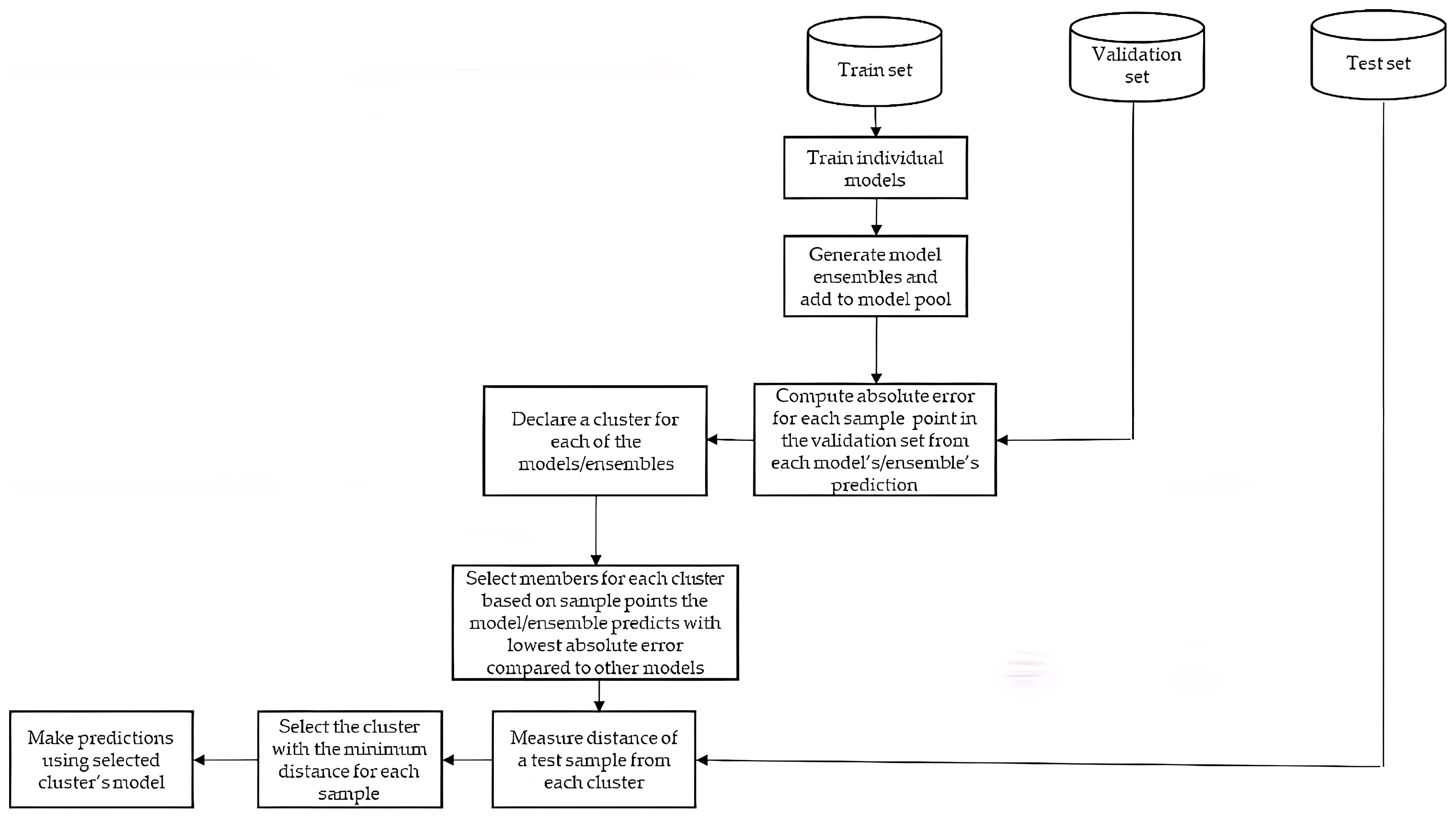
Develop a cluster for each model based on validation sample points in which they predicted with the least error. K means clustering with a K value of 1 is used for cluster formation. A value of 1 was used because the cluster members were already selected based on the minimum absolute error as shown in Figure 1, and thus, the centroids were determined by K Means. Algorithm 1, gives additional description of the DRS training phase.
Algorithm 1 Dynamic Regressor Selection Training Phase
1:
Split dataset into train, validation, and test sets with ratio 70:15:15 to obtain N t r a i n , N v a l i d a t i o n , and  N t e s t sample points, respectively.
2:
Train j models with the train set based on different algorithms with their optimized hyper-parameters to form a set Model.
3:
for i in N v a l i d a t i o n  do
4:
   for j in Model do
5:
     Compute a b s o l u t e _ e r r o r j = | P m i P p ( i j ) | , where: a b s o l u t e _ e r r o r j represent the absolute error of the jth model, P m i is the measured path loss of the ith sample point in the validation set, and  P p ( i j ) is the path loss predicted by the jth model using the ith validation sample point as input.
6:
   end for
7:
   Find m i n ( a b s o l u t e _ e r r o r )
8:
   if  m i n ( a b s o l u t e _ e r r o r ) = a b s o l u t e _ e r r o r ( j )  then
9:
     Append sample point i to cluster j
10:
   end if
11:
end for

3.1.2. Testing

(i)
Measure the distance of the test sample point to each cluster. This measures the similarity between the test sample point and validation samples in each cluster [57]. Euclidean distance is used for this purpose.
(ii)
Select the cluster with the least distance and use the model designated for the cluster to make a prediction. Further details on the DRS testing phase is presented in Algorithm 2, and description of the the whole DRS process is shown in Figure 1.
Algorithm 2 Dynamic Regressor Selection Testing Phase
1:
for k in N t e s t  do
2:
   for j in cluster do
3:
     Measure cluster distance ( d c ( j ) )
4:
   end for
5:
   Find m i n ( d c )
6:
   if  m i n ( d c ) = d c ( j )  then
7:
     Make prediction using M o d e l ( j )
8:
   end if
9:
end for represent the absolute

3.2. Dynamic Ensemble Selection (DES)

The training and testing processes in DES are the same with that of DRS described in Section 3.1.1 and Section 3.1.2. However, ensembles of models are included in addition to the single regressors/models as shown in Figure 2, which is its difference with DRS described in Figure 1. The Ensemble combinations in Table 3 were considered, and are all possible combinations of either two, three or four algorithms to exploit the accuracy improvement characteristic of ensembles resulting from the diversity provided by the base models. The DES scheme selects either a regressor or an ensemble suitable for predicting a test sample point. The ensembles are formed by averaging the predictions of the models concerned. For example, KNN+RF+GB refers to an ensemble in which the predictions of KNN, RF, and GB are summed and divided by 3.

4. Results and Discussion

The overall performance of each regressor/model, DRS and DES are examined as well as the performance per case of data.

4.1. Results Based on Dataset 1

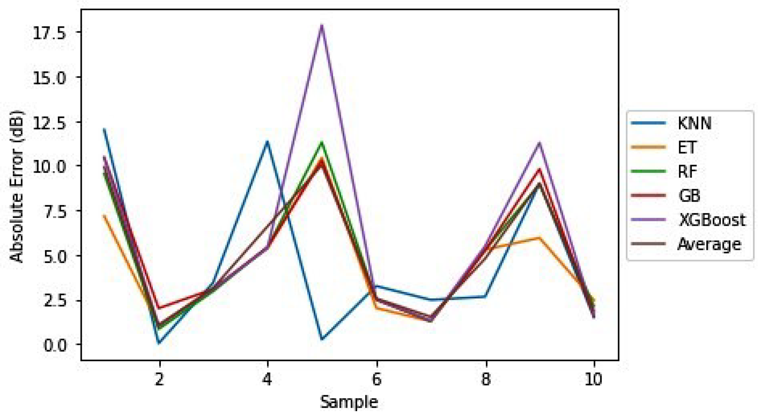
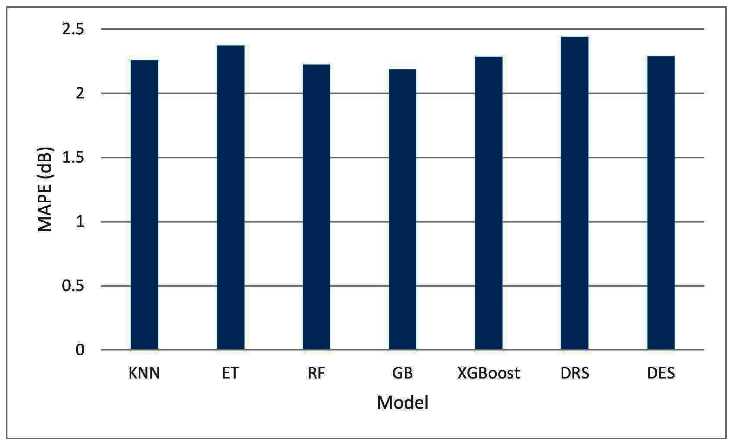
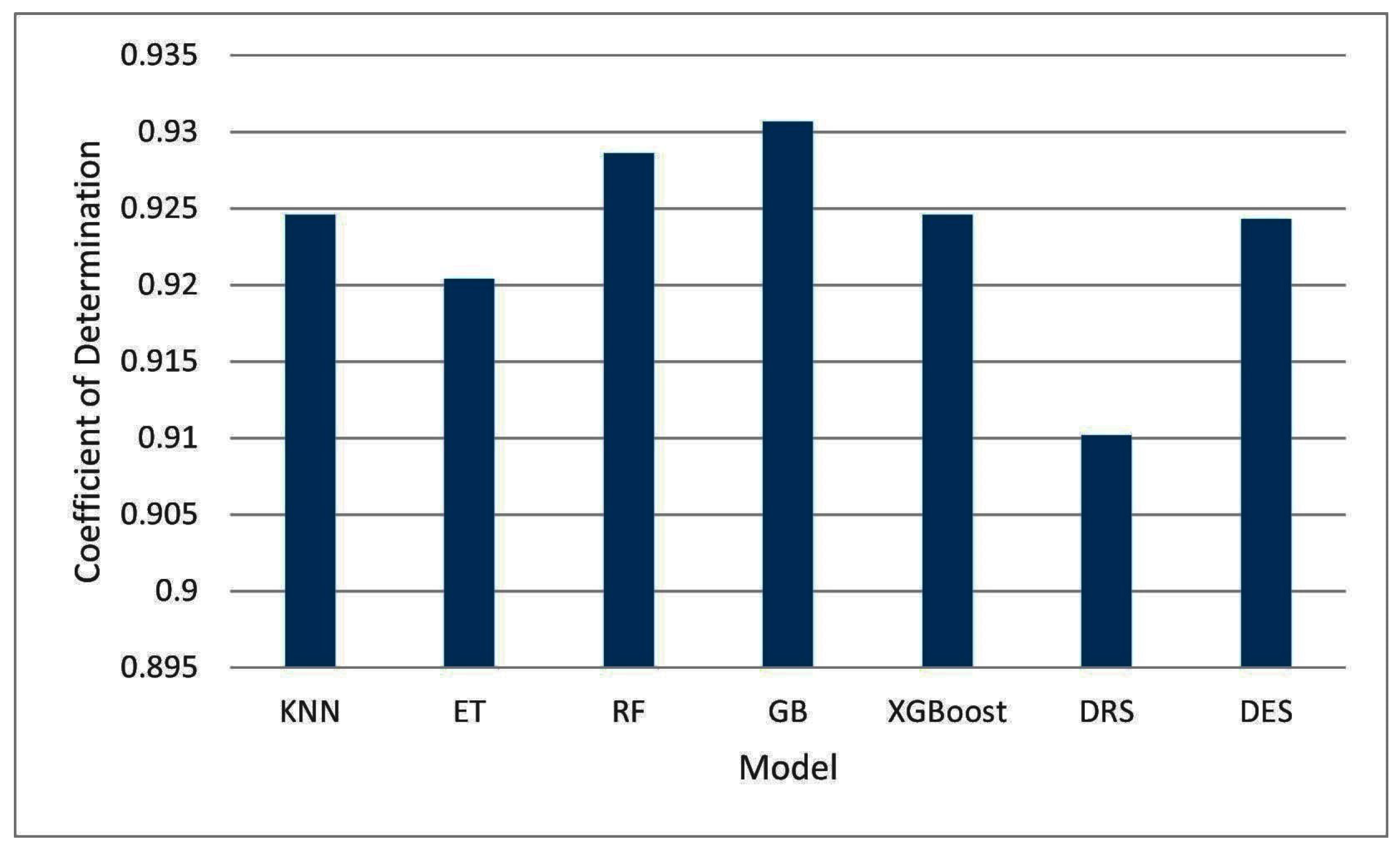
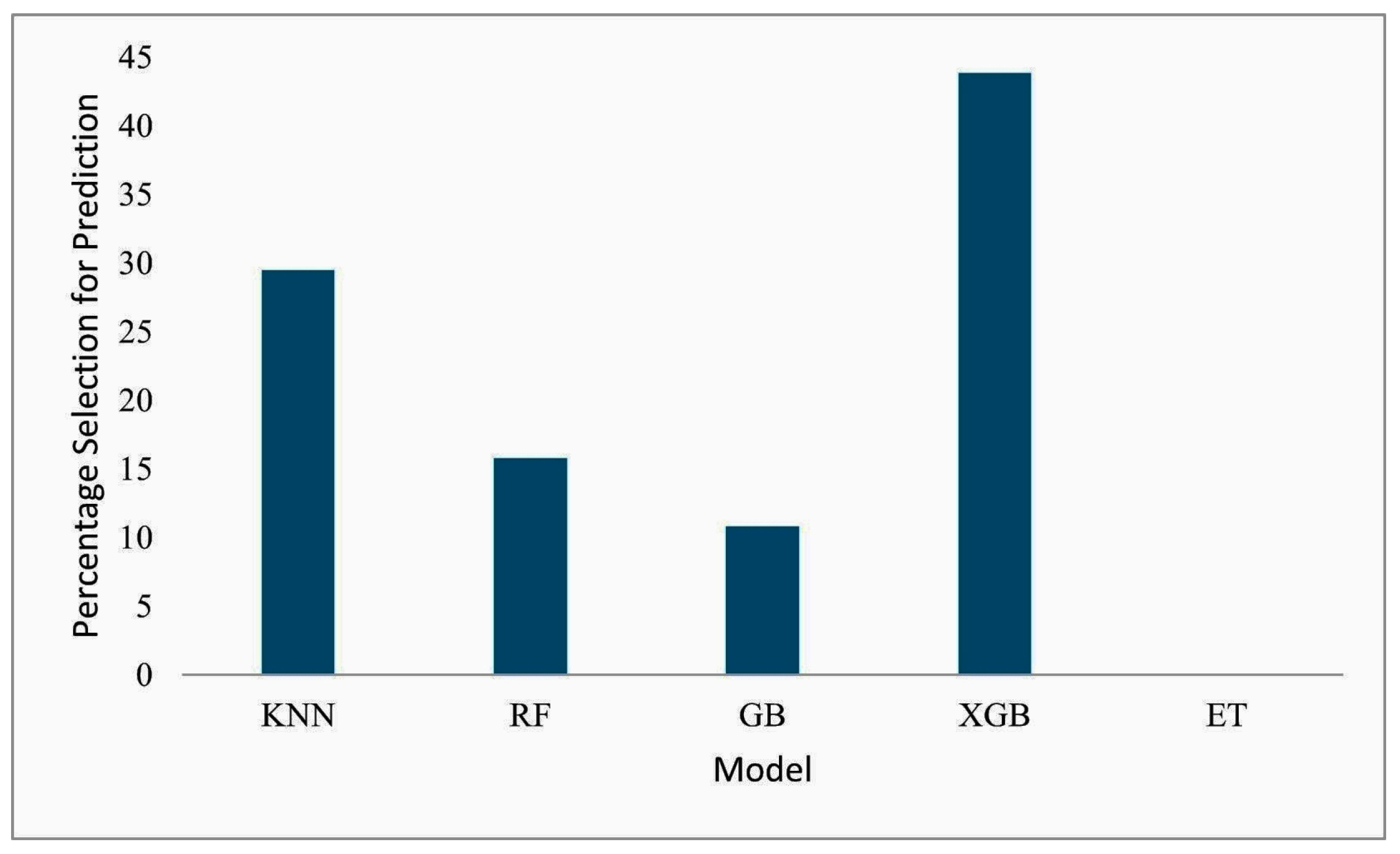
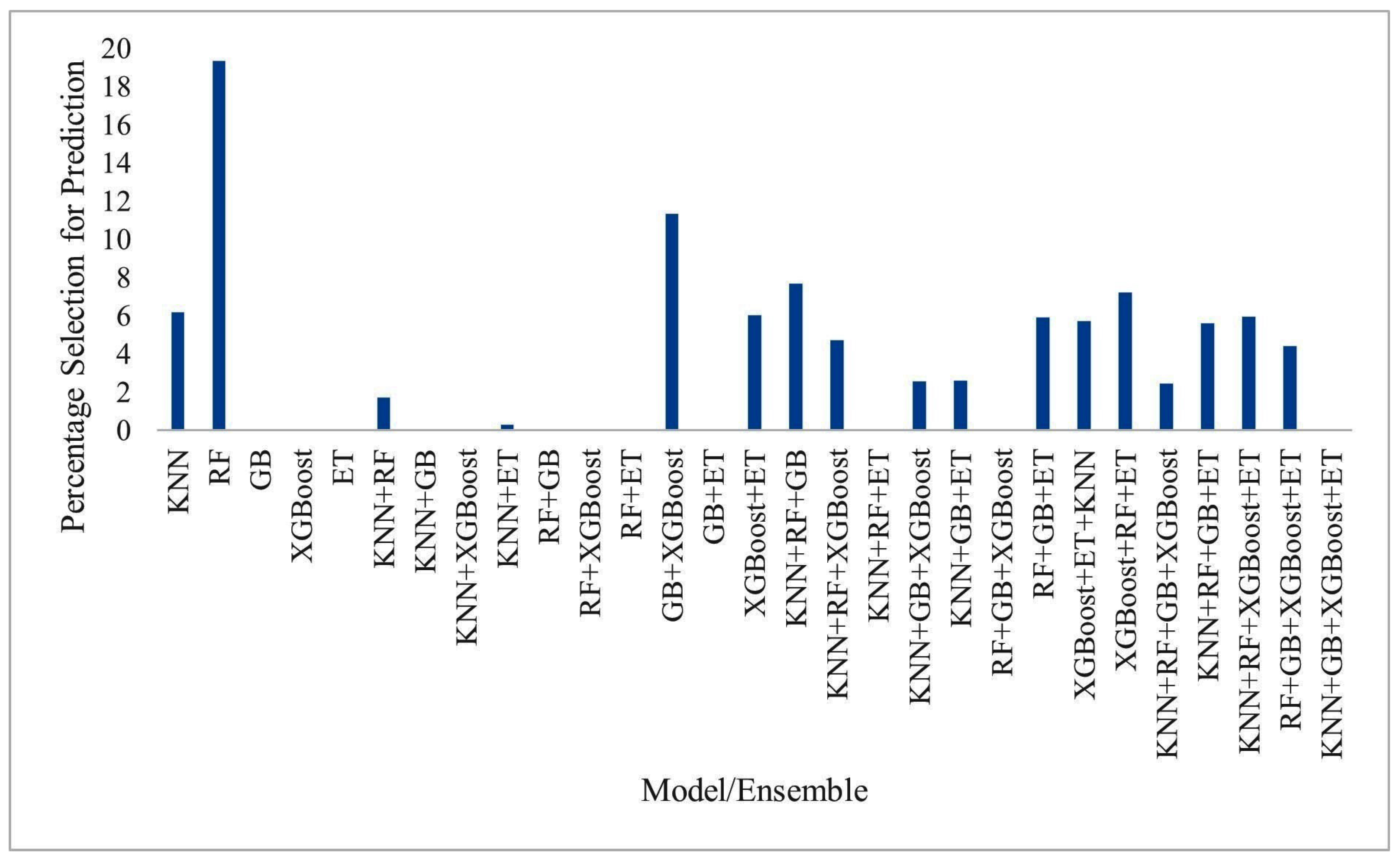
The absolute error of the various model’s predictions on 10 random sample points from the validation set are presented in Figure 3 so as to clearly show how model performance depends on individual sample points. Figure 3 shows variations in the model suitable for predicting each sample points. ET was observed to be better for the first sample point, KNN for the second, and the models performed almost equally on the third point. Likewise, there were variations in terms of the least accurate model per sample, with KNN, GB, and XGBoost having the highest absolute error for the first, second, and ninth samples, respectively. This showed that there is need to dynamically select the model/ensemble to predict each point so as to minimize the prediction error per point. Figure 4, Figure 5, Figure 6 and Figure 7 present the performance metrics in dataset 1, Figure 8 and Figure 9 present the percentage that each model/ensemble is selected for the total number of predictions made, and Table 4 shows the performance for each data case.
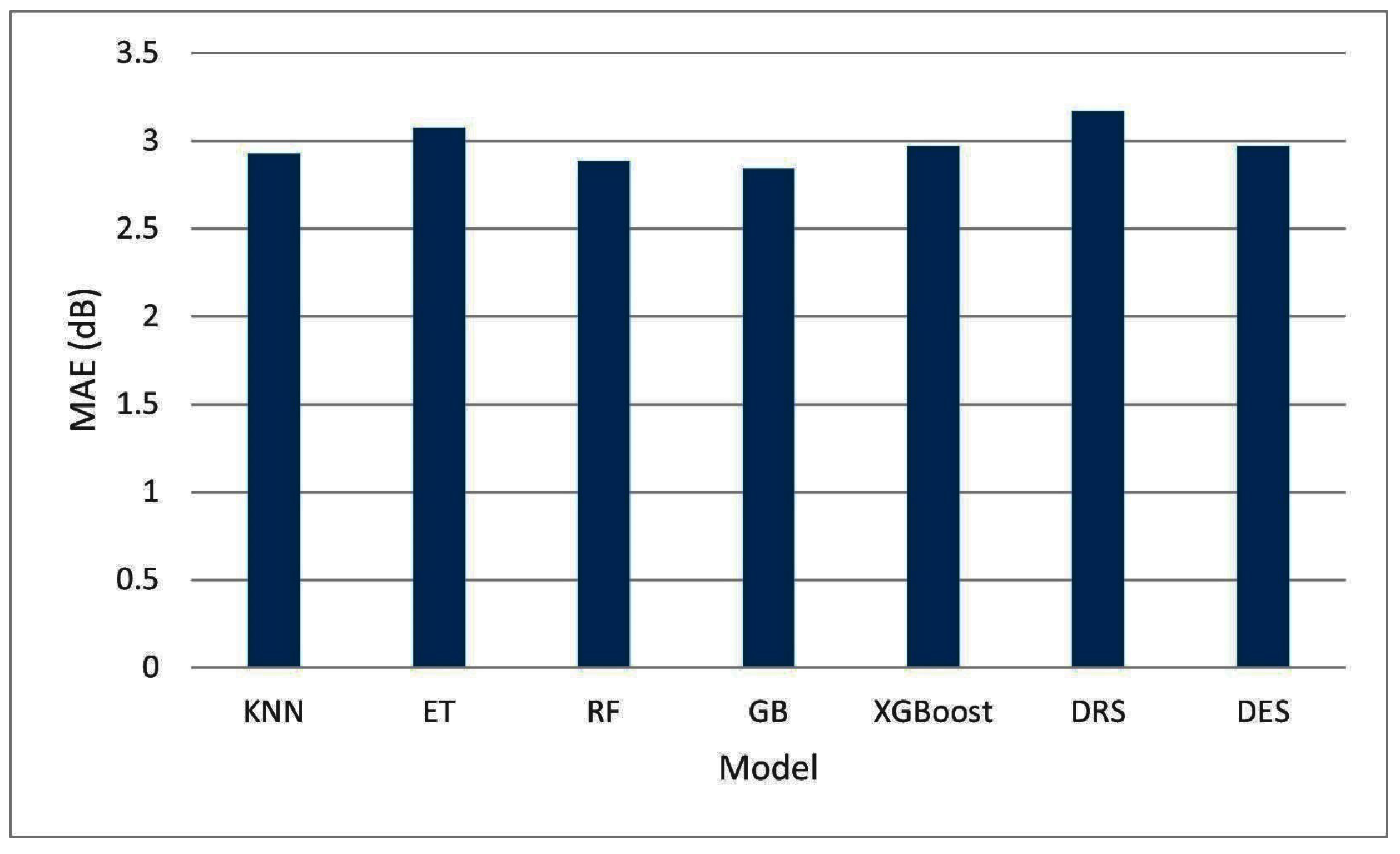
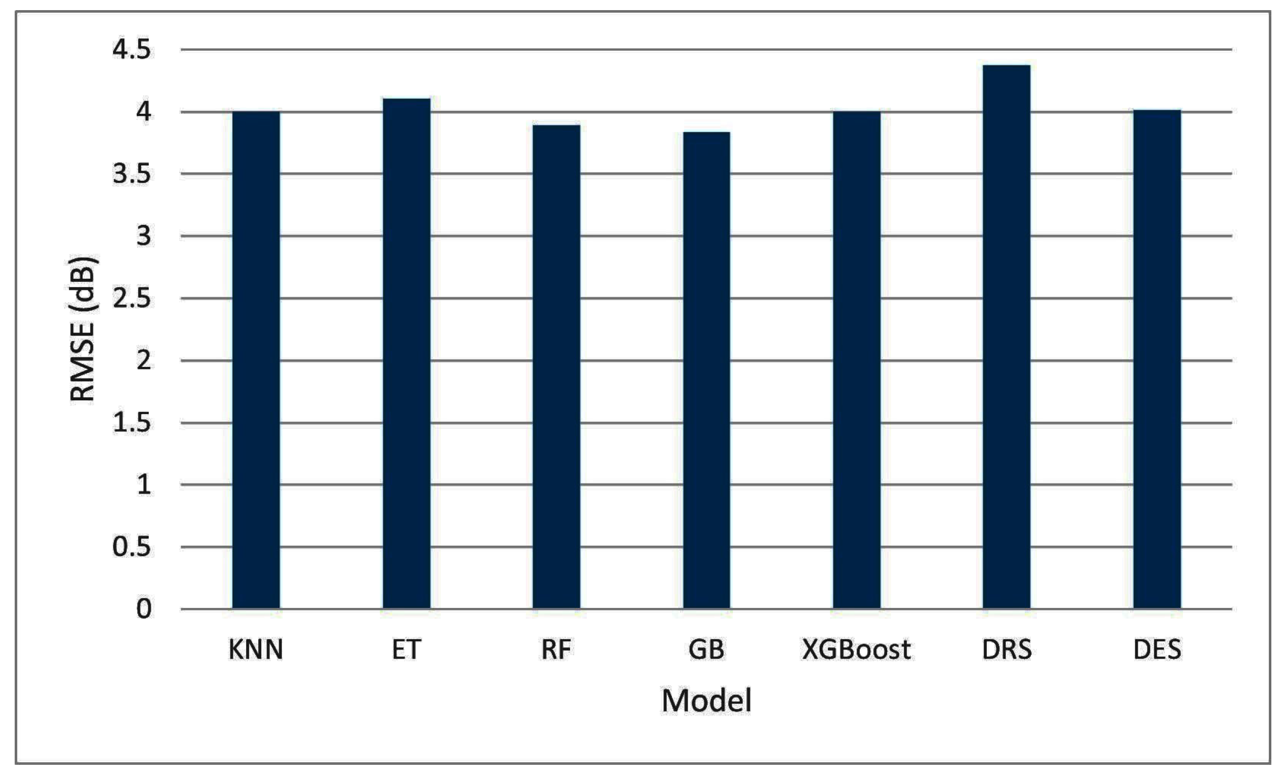
Based on the results, GB had the best overall performance as it has the least values of the error metrics and the highest Coefficient of Determination, and DRS had the least accuracy. Even though DRS and DES were not the best in terms of overall accuracy, they could be when tested on datasets in other domains [48,49].
From Table 4, it was observed that the performances in all environments and frequencies were good except in the urban at 2100 MHz band. This happened because of the few number of sample points representing the case. Although GB had the overall best accuracy based on least error and R 2 value, it was not the best in this data case as ET, RF, and DES were better than it, with ET as the best, and DRS the last. DES performance was surpassed by only ET and RF. Thus, even though it did not have the best performance, it gave an intermediary performance and could be used when avoiding the check on the individual algorithms to save time. Figure 8 shows that XGBoost was the most selected model for prediction in dataset 1 using the DRS technique, while ET is the least selected. In the case of DES in Figure 9, RF was selected the most for prediction while other single models had the least, including XGBoost that had the highest selection in DES. This showed that the ensemble of models by the combination of models in 2’s, 3’s, and 4’s, resulted in a variety of ensembles with better accuracy than the individual models and their clusters were selected for prediction due to their proximity to the sample points.
The negative coefficient of determination values for the urban environment at 2100 MHz case shows the high variation of the predicted values from the original. Under normal circumstances, it is supposed to have values between 0 and 1. However, it is negative because the Sum of Squared Error (SSE) is high to the extent that it exceeds the Total Sum of Squares as described by Equations (1)–(4). This is because the model/models learned less of this case and learned much of others, as it is represented by few sample points in the dataset.
R 2 = 1 S S E T S S
R 2 = 1 i = 1 N ( P m ( i ) P p ( i ) ) 2 i = 1 N ( P m ( i ) P p ¯ ) 2
S S E = i = 1 N ( P m ( i ) P p ( i ) ) 2
T S S = i = 1 N ( P m ( i ) P p ¯ ) 2
P m ( i ) represents the ith measured path loss, P p ( i ) the ith predicted path loss, P p ¯ the average of predicted path loss, and N the total number of observations [58].

4.2. Results Based on Dataset 2

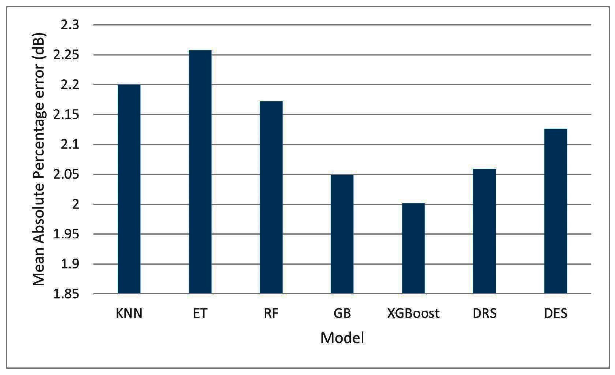
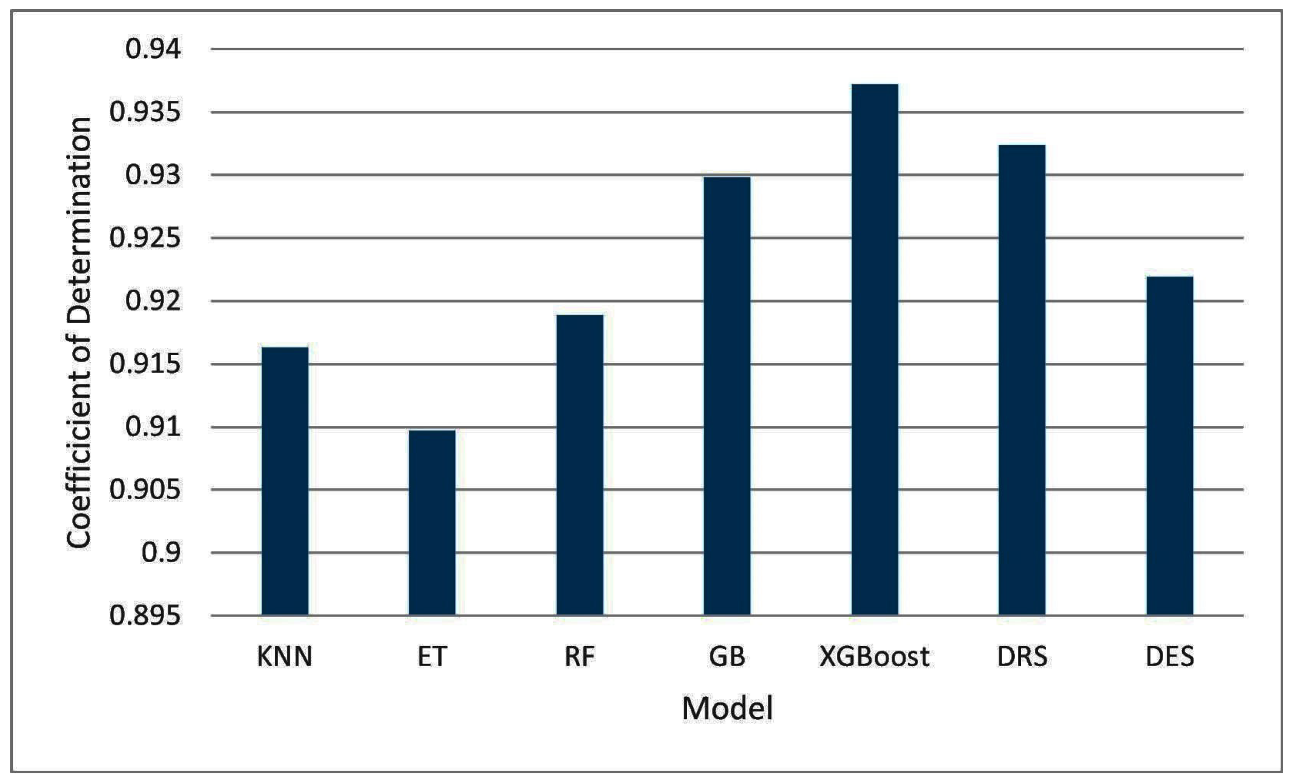
Figure 10, Figure 11, Figure 12 and Figure 13 present the performances of models on dataset 2, Figure 14 and Figure 15 present the percentage that each model/ensemble is selected for the total number of predictions made, and Table 5 shows the performance per environment case. XGBoost had the highest accuracy in this case, followed by DRS, unlike in dataset 1, where DRS had the least accuracy. This is due to the difference of the features in the two datasets. Dataset 1 has 11 features and dataset 2 has 191 features due to the presence of CNN and GLCM features extracted from satellite images which are not present in dataset 1. Each type of ML algorithm has its strengths and weaknesses. Some are good with large datasets and others are better with small datasets [59]. This caused the variation in performance of ML algorithms in the two datasets.
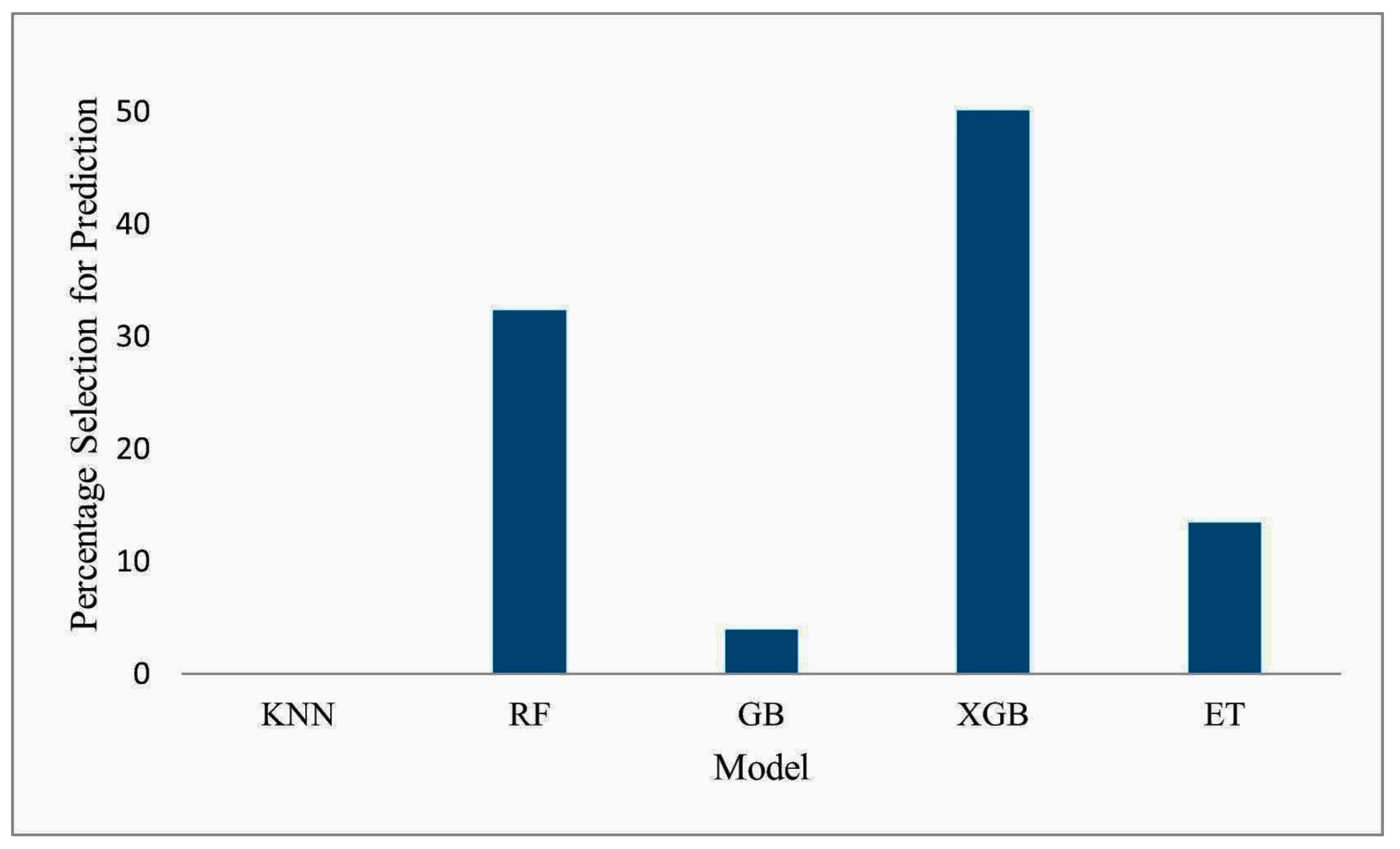
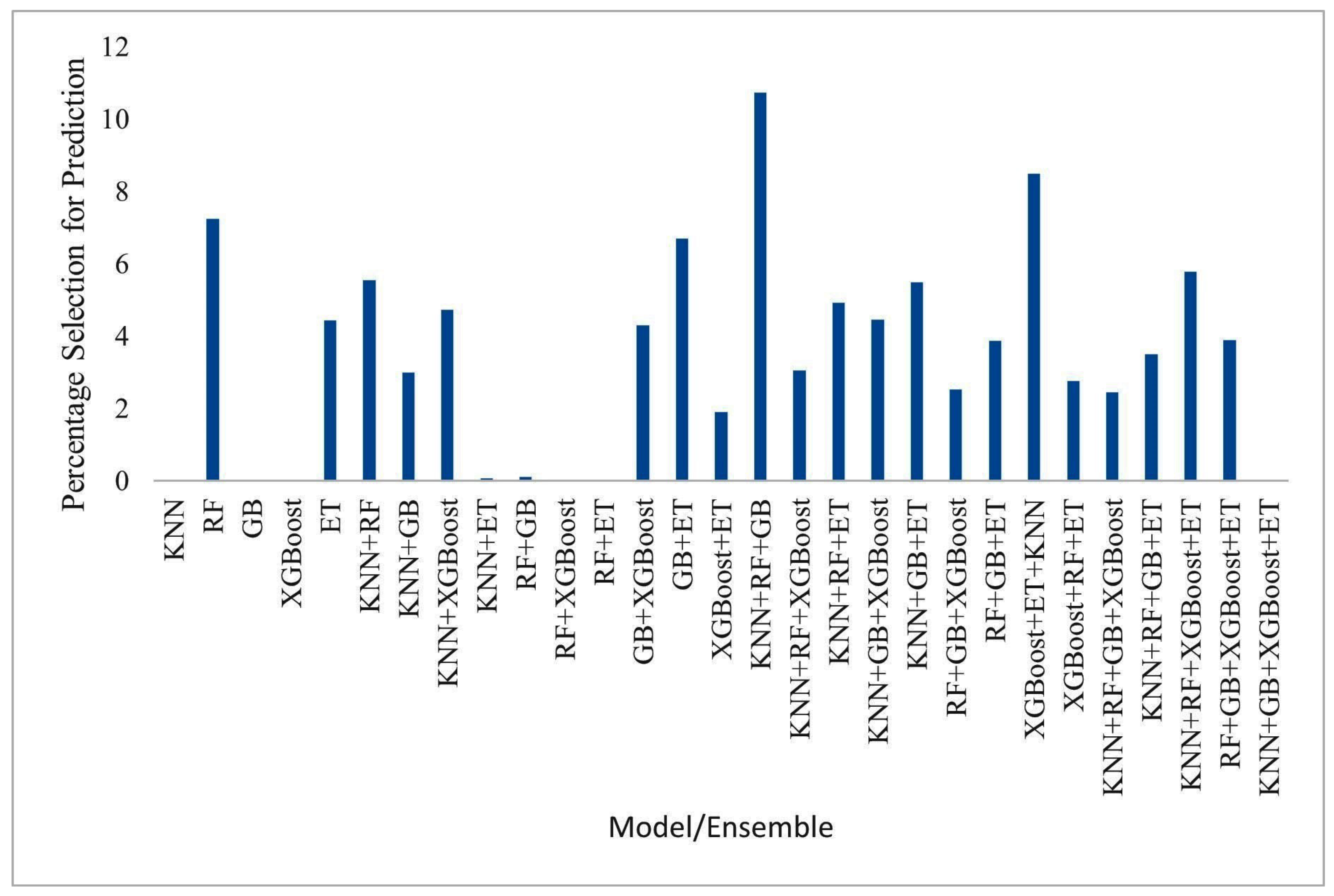
XGBoost had the overall highest accuracy and the least accurate in terms of the minority case, whereas KNN had the highest accuracy for this data case amongst the five algorithms with DRS and DES exclusive. DES had the highest accuracy with an RMSE value of 5.1577 dB for the case as it outperformed KNN (RMSE = 5.4613 dB). Thus, there was an improvement in performance in the case with the least sample points as RMSE values were below the 7 dB and 15 dB threshold values in the urban and rural environments, respectively. Although DES has higher computational complexity than the individual models, it can be used when there is imbalance in data due to its ability to select the best model/ensemble to predict for a particular test sample point. Performance based on dataset 2 is better than that of dataset 1 as observed from results obtained for the various cases of data. This is because the features in dataset 2 were rich enough to provide better description of the environments, unlike in dataset 1 where a single integer was assigned as clutter height for the environment. Figure 14 and Figure 15 present the percentage selection of the models/ensembles in dataset 2 based on DRS and DES, respectively. XGBoost was the highest selected model, and KNN was the least selected model for DRS, while an ensemble of KNN+RF+GB was the most selected in DES. DES was better than DRS in predicting the case with the least number of sample points because XGBoost was selected most in DRS. However, XGBoost has the lowest accuracy for this case (urban at band of 2100 MHz) as presented in Table 5. The addition of ensembles in DES provided more options and proper selections were made that led to improvement in prediction accuracy, unlike in DRS where there were few options.
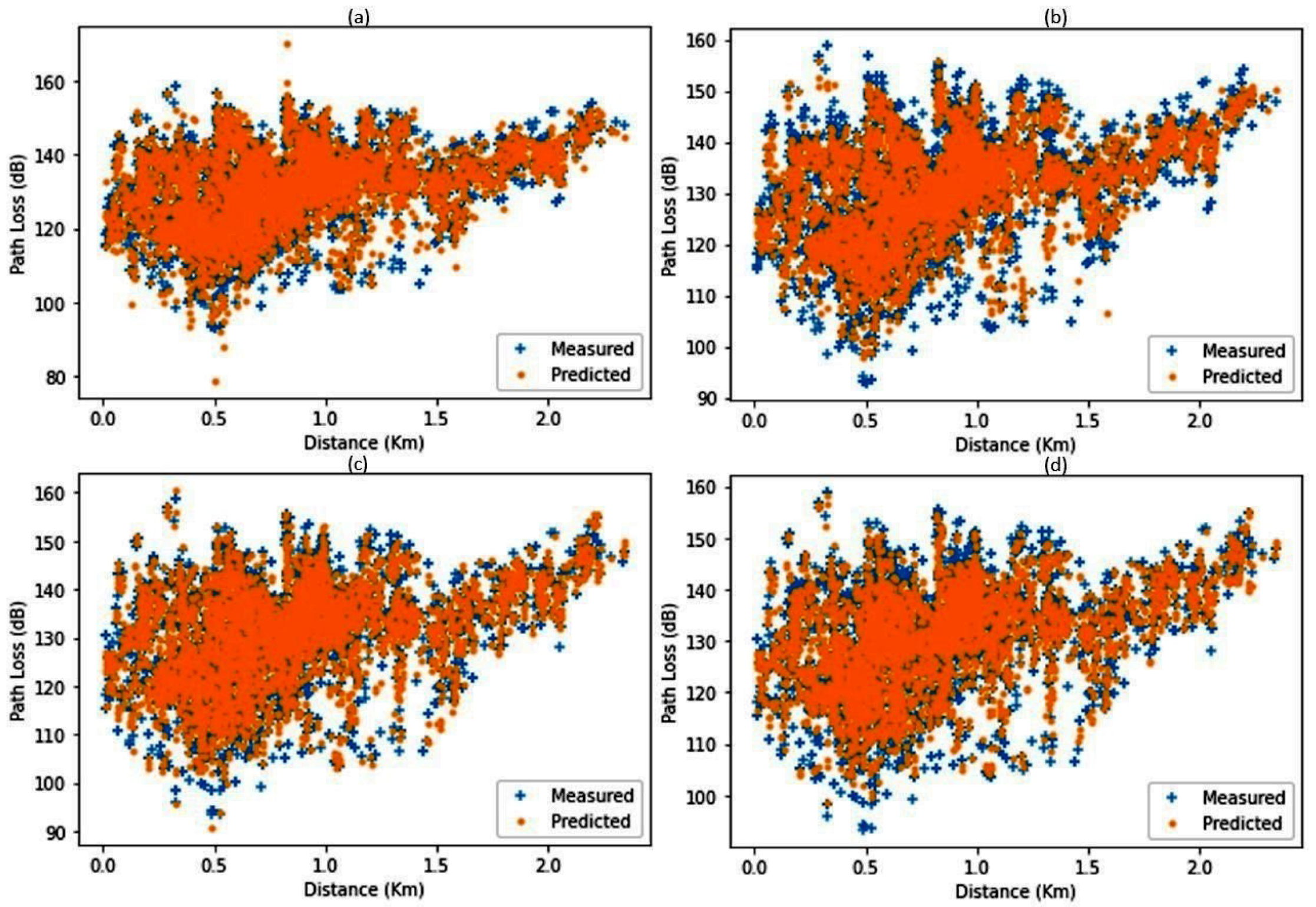
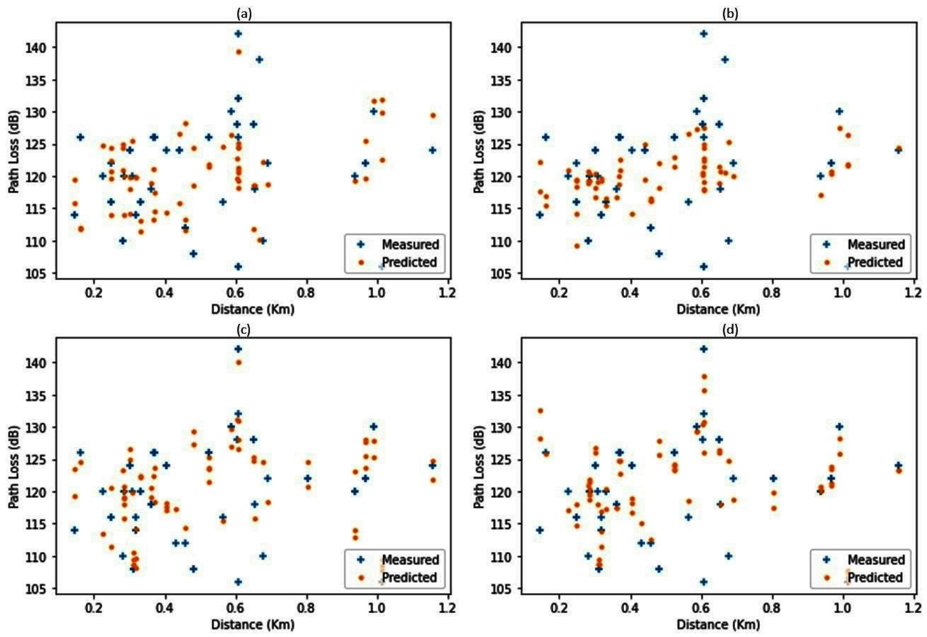
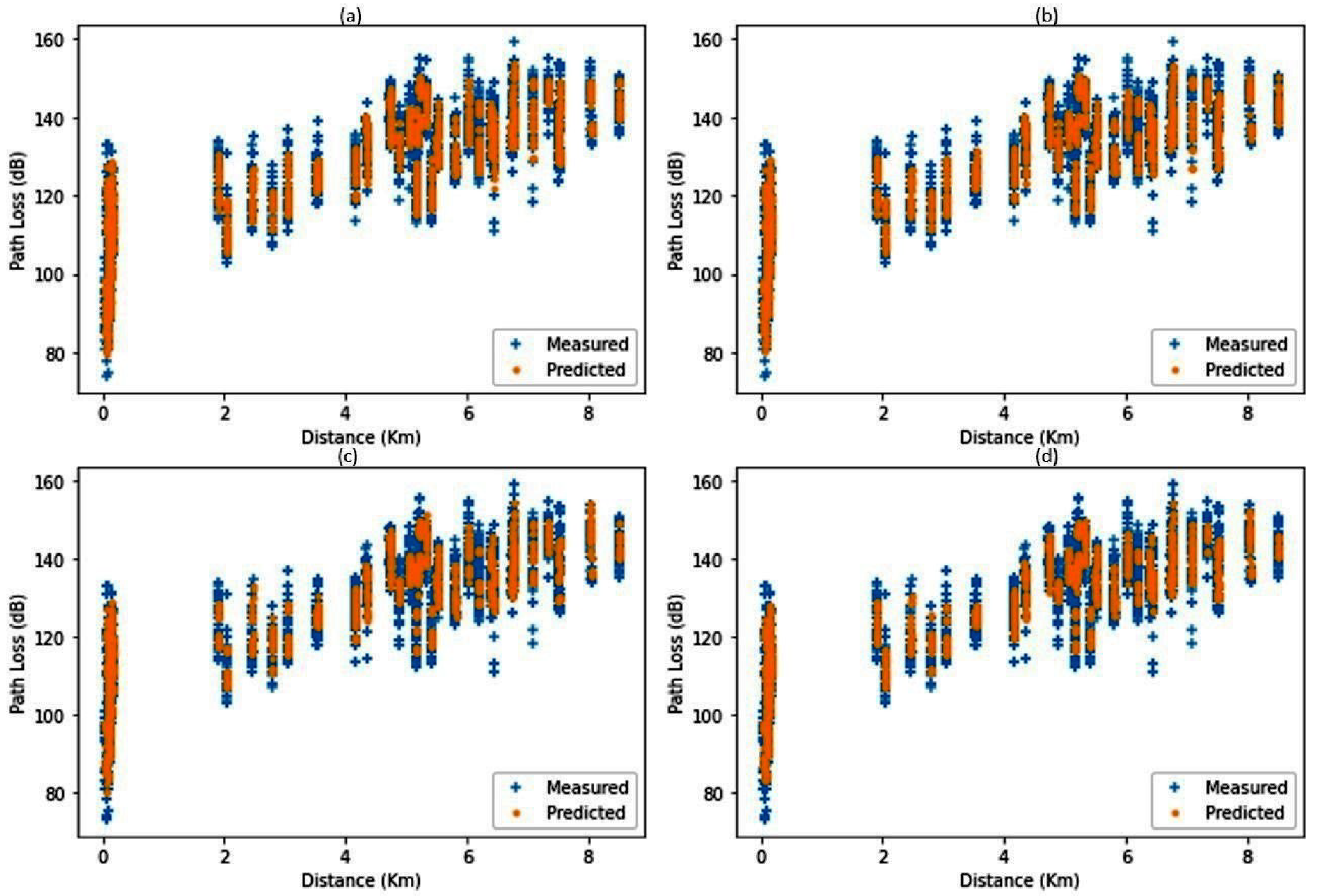
Figure 16, Figure 17, Figure 18, Figure 19 and Figure 20 present the measured and predicted path loss values versus distance by the proposed DRS and DES techniques in rural, suburban, urban at 1800 MHz, urban at 2100 MHz, and urban highrise, respectively. Good correlation between the measured and predicted path loss values was observed in all cases except for Figure 19 that represents the urban environment at the 2100 MHz band. This reflects their error metrics presented in Table 4 and Table 5. In each of the figures, not many differences were observed that will validate the preference of one technique over the other. The superiority of one over the other can only be ascertained from Table 4 and Table 5.

4.3. Comparison with Empirical Models

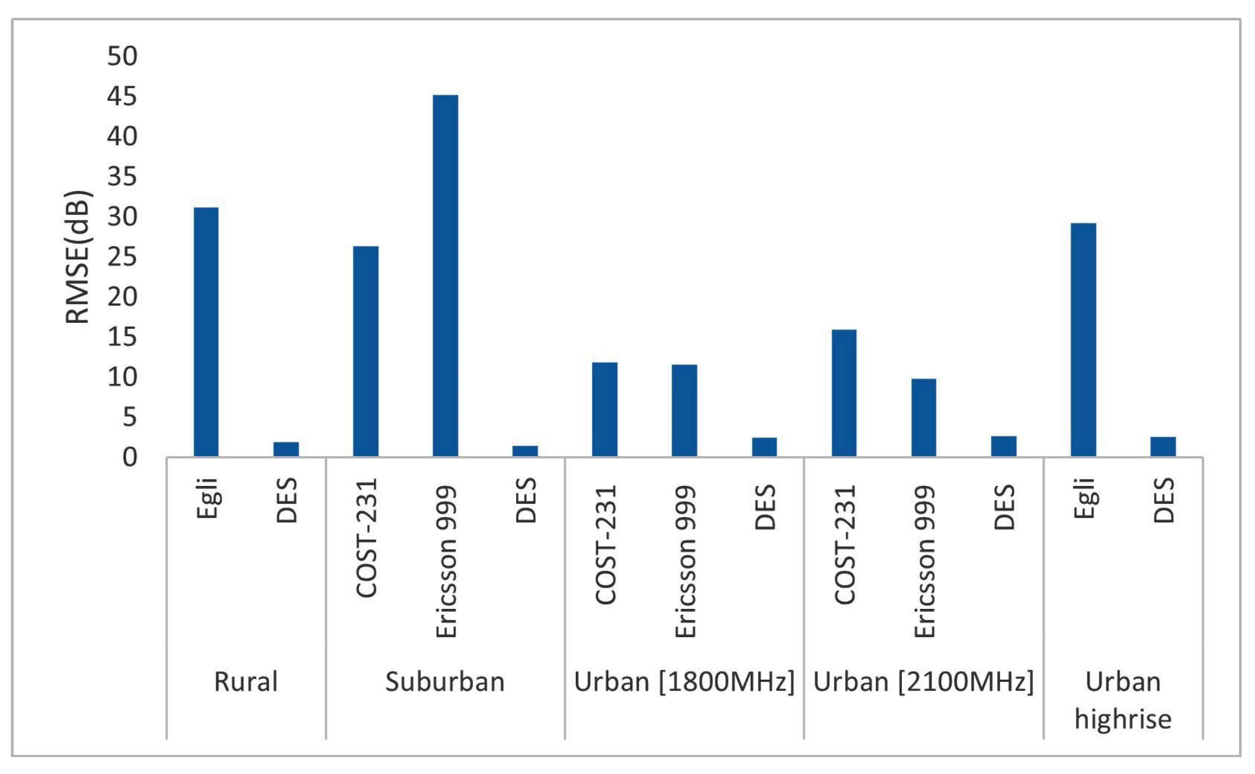
Comparison was made with the three empirical models shown in Table 6. Each of the models has a range of frequencies, antenna height, and distance within which it is valid. The Egli model was used for comparison in the rural and urban highrise environments because it is valid for 800 MHz band networks and can be used in situations where the receiving antenna height is above 10 m as in this case. Ericsson 999 and COST-231 Hata were used for suburban and urban environments because the frequency and antenna heights are within the operating ranges of the models.
Figure 21 presents performances of the empirical models in terms of RMSE in the various environments and frequency bands, and performance of the DES built from dataset 2. Comparison was done with the model developed from dataset 2 because its performance was good across the various environments and frequency bands due to the satellite image features in the dataset as well as DES ability to select the regressor/ensemble to predict a test sample point. The proposed model’s performance is better than that of the empirical models in all situations, and a wide performance gap was experienced in the rural and urban highrise environments. RMSE values of empirical models were lowest in the urban environment. The Ericsson 999 model and COST-231 Hata were lower in the urban environment than in the suburban environment. This must have been due to resemblance of environments from which the empirical models were developed with the current urban environment. The Ericsson 999 model had a better accuracy than COST-231 Hata at the two bands in the urban environment, whereas in the suburban environment, COST-231 had a better accuracy. The main determinant of the accuracy of the empirical models is the resemblance in data based on which the empirical model was developed with the data it is tested against.

4.4. Testing on Other Datasets

The proposed method was tested on datasets used in [63,64,65,66,67], and comparisons were made with results in the original works in terms of RMSE, as presented in Table 7. Although RMSE values were not presented in [65], the path loss exponent, mean, and standard deviation of the shadowing component for each of the two environments were presented. These values were substituted into the Log-distance path loss model and RMSE values of the predictions were computed. RMSE values in [63] were presented in the form of bar charts for the 811 MHz and 2630 MHz frequencies. The values were slightly above 4 dB, having approximate values of 4.25 dB and 4.1 dB, respectively. In [68], a dataset analysis was presented and the dataset was used as a subset in [66] to develop a model that resulted in an RMSE value of 6.27 dB. For the work by Carvalho et al. [67], results of 4 routes were presented, 3 of which are for suburban environments, and the fourth one is an urban environment. RMSE values for each route lies within the range 3.80 dB–6.54 dB.
Improvements were made to results in [63,65,66,67] by the proposed method and a reduction of accuracy was observed for [64] because the RMSE value was greater than that of the original work, as presented in Table 7. However, the RMSE value of 4.2061 dB by our proposed method is acceptable as it is less than 7 dB. It should be noted that results in [63,64,67] were obtained when the search space of 1:190 was used for the maximum features’ hyper-parameter in RF, ET, and GB. Meanwhile, good results were obtained from other datasets with just a search space of 1:10. Hence, the method is recommended for path loss model development, especially if the process involves combining datasets from various sources and of different settings of measurements.

5. Conclusions

Path loss models are used during the design of networks and during maintenance. Machine Learning path loss models provide predictions at a faster speed than Deterministic models without compromising accuracy. However, Deterministic models and Empirical models are adaptive to frequencies, antenna heights, and environments, while most machine learning models are developed with data from a single environment, frequency, and antenna height. Therefore, Deterministic and Empirical models have an advantage of versatility over machine learning. To develop machine learning models with such characteristics, data from various environments and with different network parameters are required. Such data can be obtained from various sources, which come in varied sizes. It is known that machine learning model performance differs on distinct parts of a dataset. Thus, this effect will be intense if several datasets were merged, as the accuracy of one of the classes in the merged dataset can be low. This was observed in the dataset used such that the accuracy of one class of the data was low compared to others. This class of data had the least size amongst the combined data. A Dynamic Regressor/Ensemble Selection model was used to solve the problem such that a model/ensemble is selected during the prediction of each data sample point. In the proposed method, a regressor/ensemble is selected to predict a sample point based on its proximity to a cluster assigned to the regressor/ensemble. The regressor/ensemble for the closest cluster is selected for prediction purposes. This improved the accuracy of the minority data class. The method’s accuracy was better than that of some empirical models it was compared against. The technique performed better when features extracted from satellite images were included compared to a case in which integer values representing clutter height were used to describe environments. Hence, the satellite image features were very qualitative for environment description which improved the minority case accuracy of the individual models, and with the Dynamic Regressor/Ensemble technique applied, the accuracy of the minority case was enhanced. The method was tested on five datasets used in other works, and an improvement in accuracy beyond that reported in the original works was observed in four out the five datasets.

Author Contributions

Conceptualization, U.S.S., D.T.C.L. and O.A.M.; methodology, U.S.S., D.T.C.L. and O.A.M.; formal analysis, U.S.S.; data curation, U.S.S.; writing—original draft preparation, U.S.S.; writing—review and editing, U.S.S., D.T.C.L. and O.A.M.; supervision, D.T.C.L. and O.A.M. All authors have read and agreed to the published version of the manuscript.

Funding

This work was funded by Universiti Brunei Darussalam, grant number RSCH/1.18/FICBF(a)/2022/004.

Data Availability Statement

The data used in this research can be provided on request.

Acknowledgments

We express our profound appreciation to Universiti Brunei Darussalam for supporting this research.

Conflicts of Interest

The authors declare no conflict of interest.

References

  1. Ibrahim, J.; Danladi, T.A.; Aderinola, M. Comparative Analysis Between Wired and Wireless Technologies in Communications: A Review. In Proceedings of the 9th IIER International Conference, Mecca, Saudi Arabia, 23–24 March 2017; pp. 45–48. [Google Scholar]
  2. Sari, A.; Alzubi, A. Path Loss Algorithms for Data Resilience in Wireless Body Area Networks for Healthcare Framework. In Security and Resilience in Intelligent Data-Centric Systems and Communication Networks, 1st ed.; Elsevier Inc.: Amsterdam, The Netherlands, 2017; pp. 285–313. [Google Scholar]
  3. Faruk, N.; Popoola, S.I.; Surajudeen-Bakinde, N.T.; Oloyede, A.A.; Abdulkarim, A.; Olawoyin, L.A.; Ali, M.; Calafate, C.T.; Atayero, A.A. Path Loss Predictions in the VHF and UHF Bands within Urban Environments: Experimental Investigation of Empirical, Heuristics and Geospatial Models. IEEE Access 2019, 7, 77293–77307. [Google Scholar] [CrossRef]
  4. Zhang, X.; Shu, X.; Zhang, B.; Ren, J.; Zhou, L.; Chen, X. Cellular Network Radio Propagation Modeling with Deep Convolutional Neural Networks. In Proceedings of the 26th ACM SIGKDD International Conference on Knowledge Discovery and Data Mining, Virtual Event, CA, USA, 6–10 July 2020; pp. 2378–2386. [Google Scholar]
  5. Mahasukhon, P.; Sharif, H.; Hempel, M.; Zhou, T.; Wang, W.; Ma, T. Propagation path loss estimation using nonlinear multi-regression approach. In Proceedings of the 2010 IEEE International Conference on Communications, Cape Town, South Africa, 23–27 May 2010. [Google Scholar]
  6. Popoola, S.I.; Oseni, O.F. Empirical Path Loss Models for GSM Network Deployment in Makurdi, Nigeria. Int. Ref. J. Eng. Sci. 2014, 3, 85–94. [Google Scholar]
  7. Ogbulezie, J.; Onuu, M. Site specific measurements and propagation models for GSM in three cities in Northern Nigeria. Am. J. Sci. Ind. Res. 2013, 4, 238–245. [Google Scholar] [CrossRef]
  8. Popoola, S.I.; Jefia, A.; Atayero, A.A.; Kingsley, O.; Faruk, N.; Oseni, O.F.; Abolade, R.O. Determination of neural network parameters for path loss prediction in very high frequency wireless channel. IEEE Access 2019, 7, 150462–150483. [Google Scholar] [CrossRef]
  9. Atoll. Atoll RF Planning and Optimisation Software User Manual, Version 3.1.0. Available online: https://www.academia.edu/9190736/Atoll_Getting_Started_UMTS_Version_3_1_0_Forsk_China (accessed on 10 June 2022).
  10. Ates, H.F.; Hashir, S.M.; Baykas, T.; Gunturk, B.K. Path Loss Exponent and Shadowing Factor Prediction From Satellite Images Using Deep Learning. IEEE Access 2019, 7, 101366–101375. [Google Scholar] [CrossRef]
  11. Ahmadien, O.; Ates, H.F.; Baykas, T.; Gunturk, B.K. Predicting Path Loss Distribution of an Area from Satellite Images Using Deep Learning. IEEE Access 2020, 8, 64982–64991. [Google Scholar] [CrossRef]
  12. Masood, U.; Farooq, H.; Imran, A. A machine learning based 3D propagation model for intelligent future cellular networks. In Proceedings of the 2019 IEEE Global Communications Conference (GLOBECOM), Waikoloa, HI, USA, 9–13 December 2019; pp. 64982–64991. [Google Scholar]
  13. Moraitis, N.; Tsipi, L.; Vouyioukas, D. Machine learning-based methods for path loss prediction in urban environment for LTE networks. In Proceedings of the 2020 16th International Conference on Wireless and Mobile Computing, Networking and Communications (WiMob), Thessaloniki, Greece, 12–14 October 2020. [Google Scholar]
  14. Abolade, R.O.; Famakinde, S.O.; Popoola, S.I.; Oseni, O.F.; Atayero, A.A.; Misra, S. Support Vector Machine for Path Loss Predictions in Urban Environment. In Computational Science and Its Applications—ICCSA 2020; Springer: Cham, Switzerland, 2020; Volume 4, pp. 995–1006. [Google Scholar]
  15. Ebhota, V.C.; Isabona, J.; Srivastava, V.M. Effect of learning rate on GRNN and MLP for the prediction of signal power loss in microcell sub-urban environment. Int. J. Commun. Antenna Propag. 2019, 9, 36–45. [Google Scholar] [CrossRef]
  16. Ojo, S.; Imoize, A.; Alienyi, D. Radial Basis Function Neural Network Path Loss Prediction Model for LTE Networks in Multitransmitter Signal Propagation Environments. Int. J. Commun. Syst. 2021, 34, e4680. [Google Scholar] [CrossRef]
  17. Singh, H.; Gupta, S.; Dhawan, C.; Mishra, A. Path Loss Prediction in Smart Campus Environment: Machine Learning-based Approaches. In Proceedings of the 2020 IEEE 91st Vehicular Technology Conference (VTC2020-Spring), Antwerp, Belgium, 25–28 May 2020. [Google Scholar]
  18. Gupta, A.; Ghanshala, K.; Joshi, R.C. Mobility Improvement by Optimizing Channel Model Coverage Through Fine Tuning. J. Cyber Secur. Mobil. 2021, 10, 593–616. [Google Scholar] [CrossRef]
  19. Omoze, E.L.; Edeko, F.O. Statistical Tuning of COST 231 Hata model in Deployed 1800MHz GSM Networks for a Rural Environment. Niger. J. Technol. 2021, 39, 1216–1222. [Google Scholar] [CrossRef]
  20. Ayadi, M.; Zineb, A.B.; Tabbane, S. A UHF Path Loss Model Using Learning Machine for Heterogeneous Networks. IEEE Trans. Antennas Propag. 2017, 65, 3675–3683. [Google Scholar] [CrossRef]
  21. Nguyen, C.; Cheema, A.A. A Deep Neural Network-based Multi-Frequency Path Loss Prediction Model from 0.8 GHz to 70 GHz. Sensors 2021, 21, 5100. [Google Scholar] [CrossRef]
  22. Sani, U.S.; Lai, D.T.C.; Malik, O.A. Investigating Automated Hyper-Parameter Optimization for a Generalized Path Loss Model. In Proceedings of the CECNet 2021; IOS Press: Amsterdam, The Netherlands, 2021; pp. 283–291. [Google Scholar]
  23. Sani, U.S.; Lai, D.T.C.; Malik, O.A. A Hybrid Combination of a Convolutional Neural Network with a Regression Model for Path Loss Prediction Using Tiles of 2D Satellite Images. In Proceedings of the 2020 8th International Conference on Intelligent and Advanced Systems (ICIAS), Kuching, Malaysia, 13–15 July 2021. [Google Scholar]
  24. Sani, U.S.; Lai, D.T.C.; Malik, O.A. Improving Path Loss Prediction Using Environmental Feature Extraction from Satellite Images: Hand-Crafted vs. Convolutional Neural Network. Appl. Sci. 2022, 12, 7685. [Google Scholar] [CrossRef]
  25. Cruz, R.M.O.; Sabourin, R. On dynamic ensemble selection and data preprocessing for multi-class imbalance learning. Int. J. Pattern Recognit. Artif. Intell. 2019, 33, 1940009. [Google Scholar] [CrossRef] [Green Version]
  26. Moura, T.J.M.; Cavalcanti, G.D.C.; Oliveira, L.S. Evaluating Competence Measures for Dynamic Regressor Selection. In Proceedings of the 2019 International Joint Conference on Neural Networks (IJCNN), Budapest, Hungary, 14–19 July 2019. [Google Scholar]
  27. García-Cano, E.; Cosío, F.A.; Duong, L.; Bellefleur, C.; Roy-Beaudry, M.; Joncas, J.; Parent, S.; Labelle, H. Dynamic ensemble selection of learner-descriptor classifiers to assess curve types in adolescent idiopathic scoliosis. Med. Biol. Eng. Comput. 2018, 56, 2221–2231. [Google Scholar] [CrossRef]
  28. Choi, Y.; Lim, D.J. DDES: A Distribution-Based Dynamic Ensemble Selection Framework. IEEE Access 2021, 9, 40743–40754. [Google Scholar] [CrossRef]
  29. Shahhosseini, M.; Hu, G.; Pham, H. Optimizing Ensemble Weights and Hyperparameters of Machine Learning Models for Regression Problems. Mach. Learn. Appl. 2022, 7, 100251. [Google Scholar] [CrossRef]
  30. Moraitis, N.; Tsipi, L.; Vouyioukas, D.; Gkioni, A.; Louvros, S. Performance evaluation of machine learning methods for path loss prediction in rural environment at 3.7GHz. Wirel. Netw. 2021, 27, 4169–4188. [Google Scholar] [CrossRef]
  31. Zhang, Y.; Wen, J.; Yang, G.; He, Z.; Wang, J. Path loss prediction based on machine learning: Principle, method, and data expansion. Appl. Sci. 2019, 9, 1908. [Google Scholar] [CrossRef] [Green Version]
  32. Zhang, Y.; Wen, J.; Yang, G.; He, Z.; Luo, X. Air-to-Air Path Loss Prediction Based on Machine Learning Methods in Urban Environments. Wirel. Commun. Mob. Comput. 2018, 2018, 8489326. [Google Scholar] [CrossRef]
  33. Wen, J.; Zhang, Y.; Yang, G.; He, Z.; Zhang, W. Path Loss Prediction Based on Machine Learning Methods for Aircraft Cabin Environments. IEEE Access 2019, 7, 159251–159261. [Google Scholar] [CrossRef]
  34. Sotiroudis, S.P.; Goudos, S.K.; Siakavara, K. Feature Importances: A Tool to Explain Radio Propagation and Reduce Model Complexity. Telecom 2020, 1, 114–125. [Google Scholar] [CrossRef]
  35. Sotiroudis, S.P.; Boursianis, A.D.; Goudos, S.K.; Siakavara, K. From Spatial Urban Site Data to Path Loss Prediction: An Ensemble Learning Approach. IEEE Trans. Antennas Propag. 2021, 70, 6–11. [Google Scholar] [CrossRef]
  36. Oroza, C.A.; Zhang, Z.; Watteyne, T.; Glaser, S.D. A Machine-Learning-Based Connectivity Model for Complex Terrain Large-Scale Low-Power Wireless Deployments. IEEE Trans. Cogn. Commun. Netw. 2017, 3, 576–584. [Google Scholar] [CrossRef]
  37. Sotiroudis, S.P.; Goudos, S.K.; Siakavara, K. Neural Networks and Random Forests: A Comparison Regarding Prediction of Propagation Path Loss for NB-IoT Networks. In Proceedings of the 2019 8th International Conference on Modern Circuits and Systems Technologies (MOCAST), Thessaloniki, Greece, 13–15 May 2019. [Google Scholar]
  38. Fujiwara, K.; Huang, Y.; Hori, K.; Nishioji, K.; Kobayashi, M.; Kamaguchi, M.; Kano, M. Over- and Under-sampling Approach for Extremely Imbalanced and Small Minority Data Problem in Health Record Analysis. Front. Public Health 2020, 8, 178. [Google Scholar] [CrossRef]
  39. Torgo, L.; Ribeiro, R.P.; Pfahringer, B.; Branco, P. SMOTE for Regression. In Progress in Artificial Intelligence; Springer International Publishing: Berlin/Heidelberg, Germany, 2013; Volume 8154. [Google Scholar]
  40. Sotiroudis, S.P.; Athanasiadou, G.; Tsoulos, G.V.; Christodoulou, C.; Goudos, S. Ensemble Learning for 5G Flying Base Station Path Loss Modelling. In Proceedings of the 2022 16th European Conference on Antennas and Propagation (EuCAP), Madrid, Spain, 27 March–1 April 2022. [Google Scholar]
  41. Branco, P.; Torgo, L.; Ribeiro, R.P. SMOGN: A Preprocessing Approach for Imbalanced Regression. In Proceedings of the First International Workshop on Learning with Imbalanced Domains: Theory and Applications, Skopje, Macedonia, 22 September 2017. [Google Scholar]
  42. Misha, J.; Shweta, M. Software Effort Estimation Using Synthetic Minority Over-Sampling Technique for Regression (SMOTER). In Proceedings of the 2022 3rd International Conference for Emerging Technology (INCET), Belgaum, India, 27–29 May 2022. [Google Scholar]
  43. Bourou, S.; El Saer, A.; Velivassaki, T.H.; Voulkidis, A.; Zahariadis, T. A Review of Tabular Data Synthesis Using GANs on an IDS Dataset. Information 2021, 12, 375. [Google Scholar] [CrossRef]
  44. Sauber-Cole, R.; Khoshgoftaar, T. The use of generative adversarial networks to alleviate class imbalance in tabular data: A survey. J. Big Data 2022, 9, 98. [Google Scholar] [CrossRef]
  45. Sotiroudis, S.P.; Siakavara, K.; Koudouridis, G.P.; Sarigiannidis, P.; Goudos, S.K. Enhancing Machine Learning Models for Path Loss Prediction Using Image Texture Techniques. IEEE Antennas Wirel. Propag. Lett. 2021, 20, 1443–1447. [Google Scholar] [CrossRef]
  46. Moraitis, N.; Tsipi, L.; Vouyioukas, D.; Gkioni, A.; Louvros, S. On the Assessment of Ensemble Models for Propagation Loss Forecasts in Rural Environments. IEEE Wirel. Commun. Lett. 2022, 11, 1097–1101. [Google Scholar] [CrossRef]
  47. Ojo, S.; Akkaya, M.; Sopuru, J.C. An ensemble machine learning approach for enhanced path loss predictions for 4G LTE wireless networks. Int. J. Commun. Syst. 2022, 35, e5101. [Google Scholar] [CrossRef]
  48. Rooney, N.; Patterson, D.; Anand, S.; Tsymbal, A. Dynamic Integration of Regression Models. In Multiple Classifier Systems, MCS 2004; Springer: Berlin/Heidelberg, Germany, 2004. [Google Scholar] [CrossRef]
  49. Rooney, N.; Patterson, D. A weighted combination of stacking and dynamic integration. Pattern Recognit. 2007, 40, 1385–1388. [Google Scholar] [CrossRef]
  50. Moura, T.J.M.; Cavalcanti, G.D.C.; Oliveira, L.S. MINE: A framework for dynamic regressor selection. Inf. Sci. 2021, 543, 157–179. [Google Scholar] [CrossRef]
  51. de, A. Cabral, J.T.H.; Oliveira, A.L.I. Ensemble Effort Estimation using dynamic selection. J. Syst. Softw. 2021, 175, 110904. [Google Scholar] [CrossRef]
  52. Rooney, N.; Patterson, D.; Tsymbal, A.; Anand, S. Random subspacing for regression ensembles. In Proceedings of the Seventeenth International Florida Artificial Intelligence Research Society, Miami Beach, FL, USA, 12–14 May 2004. [Google Scholar]
  53. Ghoneimy, S.; Faheem, M.H.; Gamal, N. Dynamic Ensemble Modelling for Prediction of Influenza Like Illnesses: A Framework. Int. J. Adv. Technol. 2020, 11, 235. [Google Scholar] [CrossRef]
  54. Dias, K.; Windeatt, T. Dynamic Ensemble Selection and Instantaneous Pruning for Regression Used in Signal Calibration. In Artificial Neural Networks and Machine Learning—ICANN 2014; Springer: Cham, Switzerland, 2014; pp. 475–482. [Google Scholar]
  55. Sun, C.; Yan, Y.; Zhang, W.; Wang, L. A Dynamic Ensemble Selection Approach to Developing Softcomputing Models for Two-Phase Flow Metering. J. Phys. Conf. Ser. 2018, 1065, 092022. [Google Scholar] [CrossRef] [Green Version]
  56. Qiao, Z.; Wang, B. Molten Steel Temperature Prediction in Ladle Furnace Using a Dynamic Ensemble for Regression. IEEE Access 2021, 9, 18855–18866. [Google Scholar] [CrossRef]
  57. Irani, J.; Pise, N.; Phatak, M. Clustering Techniques and the Similarity Measures used in Clustering: A Survey. Int. J. Comput. Appl. 2016, 134, 9–14. [Google Scholar] [CrossRef]
  58. Quddus, J. Machine Learning with Apache Spark Quick Start Guide: Uncover Patterns, Derive Actionable Insights, and Learn from Big Data Using MLlib; Packt Publishing Limited: Birmingham, UK, 2018. [Google Scholar]
  59. Namoun, A.; Hussein, B.R.; Tufail, A.; Alrehaili, A.; Syed, T.A.; Benrhouma, O. An Ensemble Learning Based Classification Approach for the Prediction of Household Solid Waste Generation. Sensors 2022, 22, 3506. [Google Scholar] [CrossRef]
  60. Jawhly, T.; Tiwari, R.C. Characterization of path loss for VHF terrestrial band in Aizawl, Mizoram (India). In Engineering Vibration, Communication and Information Processing; Springer Nature: Singapore, 2019; pp. 53–63. [Google Scholar]
  61. Opio, P.; Kisolo, A.; Ireeta, T.W.; Okullo, W. Modeling the Distribution of Radiofrequency Intensities from the Digital Terrestrial Television (DTTV) Broadcasting Transmitter in Kampala. Asian J. Res. Rev. Phys. 2020, 3, 65–78. [Google Scholar] [CrossRef]
  62. Türke, U. Efficient Methods for WCDMA Radio Network Planning and Optimization; Deutscher Universitätsverlag: Wiesbaden, Germany, 2007. [Google Scholar]
  63. Thrane, J.; Zibar, D.; Christiansen, H.L. Model-aided deep learning method for path loss prediction in mobile communication systems at 2.6 GHz. IEEE Access 2020, 8, 7925–7936. [Google Scholar] [CrossRef]
  64. Timoteo, R.D.A.; Cunha, D.C.; Cavalcanti, G.D.C. A Proposal for Path Loss Prediction in Urban Environments Using Support Vector Regression. In Proceedings of the Tenth Advanced International Conference on Telecommunications, Paris, France, 20–24 July 2014; pp. 119–124. [Google Scholar]
  65. Chall, R.E.; Lahoud, S.; Helou, M.E. LoRaWAN Network Radio Propagation Models and Performance Evaluation in Various Environments in Lebanon. IEEE Internet Things J. 2019, 6, 2366–2378. [Google Scholar] [CrossRef]
  66. Popoola, S.I.; Adetiba, E.; Atayero, A.A.; Faruk, N.; Calafate, C.T. Optimal model for path loss predictions using feed-forward neural networks. Cogent Eng. 2018, 5, 1. [Google Scholar] [CrossRef]
  67. Carvalho, A.A.P.D.; Batalha, I.S.; Neto, M.A.; Castro, B.L.; Barros, F.J.B. Adjusting Large-Scale Propagation Models for the Amazon Region Using Bioinspired Algorithms at 1.8 and 2.6 GHz Frequencies. J. Microw. Optoelectron. Electromagn. Appl. 2021, 20, 445–463. [Google Scholar] [CrossRef]
  68. Popoola, S.I.; Atayero, A.A.; Arausi, O.D.; Matthews, V.O. Path loss Dataset for Modeling Radio Wave Propagation in Smart Campus Environment. Data Br. 2018, 17, 1062–1073. [Google Scholar] [CrossRef]
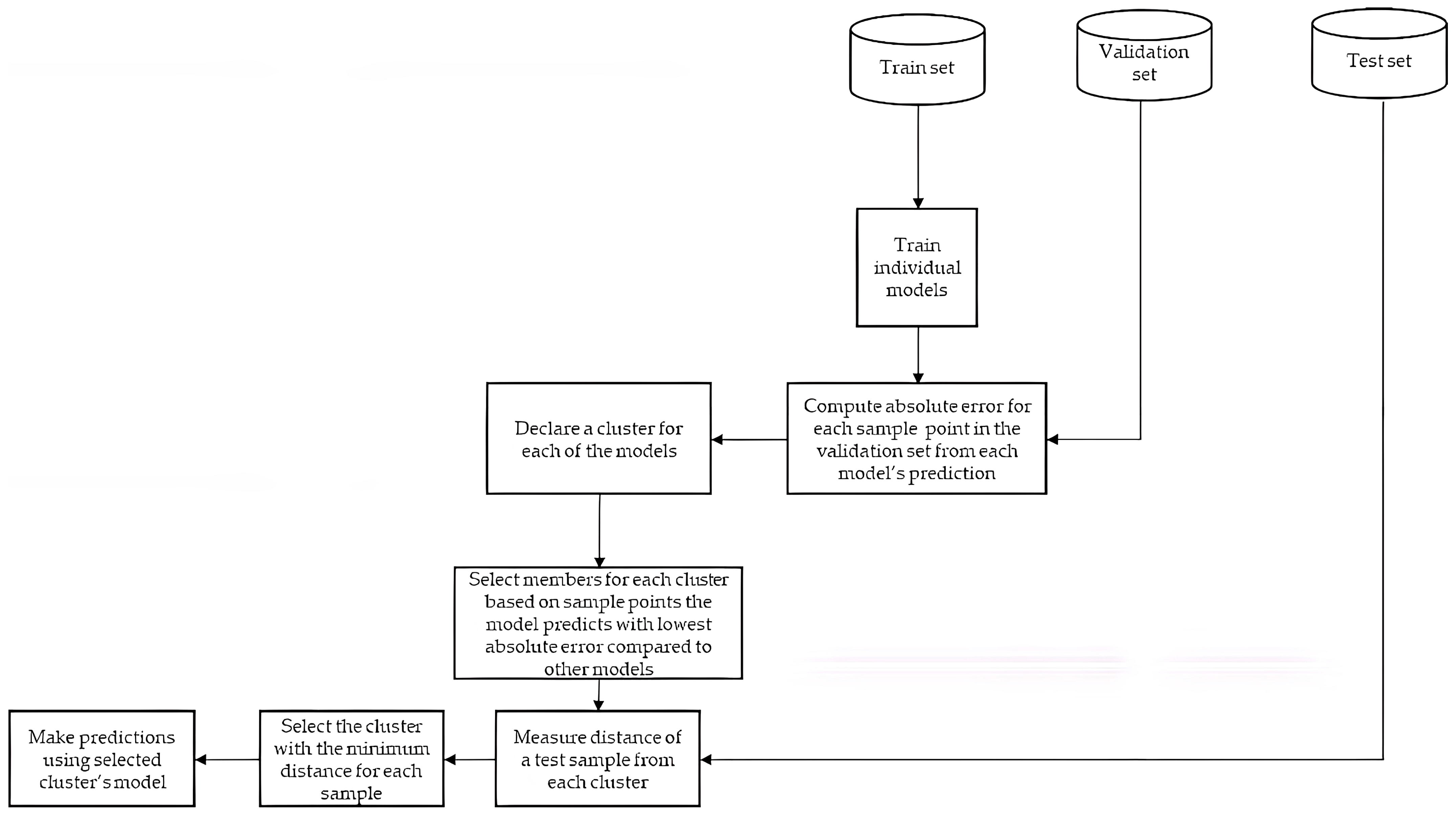
Figure 1. Dynamic Regressor Selection Process.
Information 13 00519 g001
Figure 2. Dynamic Ensemble selection process.
Information 13 00519 g002
Figure 3. Absolute error of sample points in the validation set.
Information 13 00519 g003
Figure 4. Mean Absolute Error values of models based on dataset 1.
Information 13 00519 g004
Figure 5. Root Mean Squared Error of models based on dataset 1.
Information 13 00519 g005
Figure 6. Mean Absolute Percentage Error of models based on dataset 1.
Information 13 00519 g006
Figure 7. Coefficient of determination of models from dataset 1.
Information 13 00519 g007
Figure 8. Percentage of model selection in DRS for dataset 1.
Information 13 00519 g008
Figure 9. Percentage of model/ensemble selection in DES for dataset 1.
Information 13 00519 g009
Figure 10. Mean Absolute Error values of models based on dataset 2.
Information 13 00519 g010
Figure 11. Root Mean Squared Error of models based on dataset 2.
Information 13 00519 g011
Figure 12. Mean Absolute Percentage Error of models based on dataset 2.
Information 13 00519 g012
Figure 13. Coefficient of determination of models from dataset 2.
Information 13 00519 g013
Figure 14. Percentage of model selection in DRS for dataset 2.
Information 13 00519 g014
Figure 15. Percentage of model/ensemble selection in DES for dataset 2.
Information 13 00519 g015
Figure 16. Predictions in rural environment based on (a) DRS on dataset 1, (b) DES on dataset 1, (c) DRS on dataset 2, (d) DES on dataset 2.
Information 13 00519 g016
Figure 17. Predictions in suburban environment based on (a) DRS on dataset 1, (b) DES on dataset 1, (c) DRS on dataset 2, (d) DES on dataset 2.
Information 13 00519 g017
Figure 18. Predictions in urban (1800 MHz) environment based on (a) DRS on dataset 1, (b) DES on dataset 1, (c) DRS on dataset 2, (d) DES on dataset 2.
Information 13 00519 g018
Figure 19. Predictions in urban (2100 MHz) environment based on (a) DRS on dataset 1, (b) DES on dataset 1, (c) DRS on dataset 2, (d) DES on dataset 2.
Information 13 00519 g019
Figure 20. Predictions in urban highrise environment based on (a) DRS on dataset 1, (b) DES on dataset 1, (c) DRS on dataset 2, (d) DES on dataset 2.
Information 13 00519 g020
Figure 21. RMSE values of empirical models in various environments.
Information 13 00519 g021
Table 2. Summary of datasets.
DatasetSizeFeatures
Dataset 112,369Distance, elevation of transmitter position, elevation of receiver position, frequency, height of transmitting antenna, height of receiving antenna, clutter height, latitude, longitude, distance in latitude between transmitting and receiving antenna, and distance in longitude between transmitting and receiving antenna.
Dataset 212,369Distance, elevation of transmitter position, elevation of receiver position, frequency, height of transmitting antenna, height of receiving antenna, distance in latitude between transmitting and receiving antenna, distance in longitude between transmitting and receiving antenna, and others extracted from satellite images using a CNN and GLCM.
Table 3. Ensemble combinations.
Two AlgorithmsThree AlgorithmsFour Algorithm
KNN+RFKNN+RF+GBKNN+RF+GB+XGBoost
KNN+GBKNN+RF+XGBoostKNN+RF+GB+ET
KNN+XGBoostKNN+RF+ETKNN+RF+XGBoost+ET
KNN+ETKNN+GB+XGBoostKNN+GB+XGBoost+ET
RF+GBKNN+GB+ETRF+GB+XGBoost+ET
RF+XGBoostRF+GB+XGBoost
RF+ETRF+GB+ET
GB+XGBoostXGBoost+ET+KNN
GB+ETXGBoost+RF+ET
XGBoost+ET
Table 4. Performance on the different cases in dataset 1.
AlgorithmEnvironmentBandMAE (dB)RMSE (dB)MAPE (dB) R 2
KNNAllAll2.92753.99982.25830.9246
Rural8002.71443.70262.13300.9426
Suburban18002.28623.08391.61920.8822
Urban18003.46954.51892.70690.8324
Urban21006.53018.11025.5187−0.1391
Urban highrise8003.21474.43962.59110.9164
ETAllAll3.07454.10782.37080.9204
Rural8002.57123.46932.02200.9496
Suburban18002.71023.58571.92390.8409
Urban18003.76664.86192.95310.8060
Urban21006.22947.69685.2703−0.0265
Urban highrise8003.11454.20432.52880.9251
RFAllAll2.88153.89082.22170.9286
Rural8002.57063.46232.02310.9483
Suburban18002.32803.14571.65240.8775
Urban18003.56184.56812.78330.8287
Urban21006.38817.71695.3807−0.0317
Urban highrise8003.03754.16772.44740.9263
GBAllAll2.84263.83502.18670.9307
Rural8002.53103.44431.99020.9504
Suburban18002.35293.13451.66690.8784
Urban18003.37234.32392.6240.8465
Urban21006.62648.05655.6001−0.1262
Urban highrise8003.04864.18662.45590.9257
XGBoostAllAll2.96903.99832.28510.9246
Rural8002.54503.43362.00230.9498
Suburban18002.51503.35661.78240.8605
Urban18003.61794.66632.81940.8212
Urban21006.52898.08225.5532−0.1364
Urban highrise8003.11124.22270.51100.9244
DRSAllAll3.16924.37572.43960.9102
Rural8002.72583.73402.13390.9386
Suburban18002.59773.68921.84640.8342
Urban18004.06725.32603.17170.7665
Urban21008.991210.86777.5460−0.4363
Urban highrise8003.25884.48082.61390.9139
DESAllAll2.96774.01452.28650.9243
Rural8002.50013.39011.95990.9494
Suburban18002.51733.41731.78870.8579
Urban18003.63564.70482.84840.8178
Urban21008.00069.62306.7360−0.1095
Urban highrise8003.23264.43352.58640.9156
Table 5. Performance on the different cases in dataset 2.
AlgorithmEnvironmentBandMAE (dB)RMSE (dB)MAPE (dB) R 2
KNNAllAll2.83284.23072.19970.9163
Rural8003.22763.24291.91160.9572
Suburban18003.24292.73571.42740.9085
Urban18003.59795.73362.81390.7278
Urban21003.26225.46132.85400.5099
Urban highrise8003.22764.39352.60340.9151
ETAllAll2.90584.36272.25770.9097
Rural8002.57863.38852.04770.9533
Suburban18002.04812.75671.45060.9071
Urban18003.47085.84602.70770.7171
Urban21003.63486.05123.15110.3940
Urban highrise8003.50894.75022.82890.9007
RFAllAll2.80864.15842.17210.9189
Rural8002.47533.34401.94600.9525
Suburban18002.16552.89481.53500.9006
Urban18003.38665.35202.64530.7589
Urban21004.47506.29593.74030.2986
Urban highrise8003.11174.29892.49690.9199
GBAllAll2.64853.84592.04910.9298
Rural8002.38763.24061.88020.9573
Suburban18002.05172.75991.45520.9068
Urban18003.08064.75842.40960.8125
Urban21003.95866.42573.43430.3257
Urban highrise8003.09384.27692.48100.9195
XGBoostAllAll2.58483.66802.00130.9372
Rural8002.43843.26221.92010.9557
Suburban18001.93142.63621.36750.9150
Urban18003.59755.48512.81290.7509
Urban21005.03996.76894.24410.2529
Urban highrise8003.10884.26392.49140.9200
DRSAllAll2.65933.78062.05890.9324
Rural8002.55773.40032.02960.9481
Suburban18001.98432.67241.40270.9096
Urban18002.83814.17502.20910.8469
Urban21003.87185.67923.32680.5023
Urban highrise8003.18154.45012.55330.9129
DESAllAll2.74524.06312.12620.9219
Rural8002.44463.28961.93070.9514
Suburban18002.02172.70291.42850.9076
Urban18003.17495.07922.47510.7732
Urban21003.09245.15772.66250.5885
Urban highrise8003.21384.44602.58600.9131
Table 6. Empirical models and their input parameter limit.
Empirical ModelFrequency Range (MHz)Transmitting Antenna Height Range (m)Receiving Antenna Height Range (m)Distance Range (km)
Egli [60][40, 1000]n/a 10 and 10[1, 80]
Ericsson 999 [61][150, 1900][30, 300][1, 10][1, 20]
COST-231 Hata [62][1500, 2000][30, 200][1, 10][1, 20]
Table 7. Performance of proposed method on other datasets.
DatasetRMSE in Original Work (dB)RMSE with Proposed DES Method (dB)
[63] at 811 MHz≈4.10003.4420
[63] at 2630 MHz≈4.25002.2058
[64]1.76004.2061
[65] for Rural10.28443.2203
[65] for Urban highrise6.43004.3679
[66,68]6.27002.6780
[67]3.8000–6.54003.2415–5.1490
Publisher’s Note: MDPI stays neutral with regard to jurisdictional claims in published maps and institutional affiliations.