Fuzzy Spatiotemporal Data Modeling and Operations in RDF

Abstract

With the emergence of a large number of fuzzy spatiotemporal data on the Web, how to represent and operate fuzzy spatiotemporal data has become an important research issue. Meanwhile, the Resource Description Framework (RDF) is a standard data and knowledge description language of the Semantic Web and has been applied in many application areas, such as geographic information systems and meteorological systems. In this paper, a model for representing fuzzy spatiotemporal data is proposed and a set of algebraic operations for the model are investigated. First, a representation method of fuzzy spatiotemporal RDF data and a fuzzy spatiotemporal RDF graph model are proposed. In addition, a formal fuzzy spatiotemporal RDF algebra is proposed and a set of algebraic operations for manipulating fuzzy spatiotemporal RDF data are developed. The algebraic operations include: set operation, selection operation, projection operation, join operation, and construction operation. Finally, the existing SPARQL query language is extended and an example that shows how to apply the proposed algebraic operations to capture the queries expressed by the extended SPARQL query language is given.

1. Introduction

The Resource Description Framework (RDF) is a standard metadata model recommended by the World Wide Web Consortium (W3C) for representing the resource information on the Semantic Web. Due to its universality and flexibility, the RDF is assuming an undeniably significant part in different fields, such as biological networks [1], the social Web [2], large-scale knowledge bases [3], and more generally, as a light-weight representation of the “Web of data” [4]. It has turned into an overall calculated portrayal or displaying method. According to a specialized perspective, an RDF database is an assortment of triples. Each triple is presented as (subject, predicate, object), which describes the property value of the subject or the relation between the two entities—the subject and the object. RDF databases can also be viewed as labeled directed graphs due to their homogeneous structure, where vertices represent subjects and objects, and edges represent predicates connecting from subject vertices to object vertices.

However, in many real-world applications, a huge amount of entities and statements contain spatial and temporal information [5,6,7,8,9], and information is often fuzzy. For instance, in the meteorological framework, the area of a storm can change after some time, which mirrors its spatiotemporal qualities, and its boundary cannot be accurately determined, which reflects its fuzzy characteristics. Sadly, the straightforward RDF triples could not address such data. Accordingly, it is important to extend the design of the RDF model to express fuzzy spatiotemporal information.

Currently, several extensions of the RDF are proposed to manage spatiotemporal information and fuzzy information [10,11,12,13,14,15,16,17,18]. Theocharidis et al. [10] propose a general coding scheme for managing the spatial RDF data effectively. Gutierrez et al. [11] present a framework that incorporates temporal reasoning into RDF. Fu Zhang et al. [12] propose a model for representing temporal data based on RDF. Additionally, there are initiatives to incorporate temporal and spatial features into a modeling framework. For example, Wang et al. [13] proposed an approach for querying large spatiotemporal RDF graphs. Del Mondo et al. [14] introduced a graph-based method for representing changing objects through time and space. In the field of fuzzy RDF, there are also RDF extensions that represent fuzzy information. Straccia et al. [15] exhibited the fuzzy RDF in a generic context where comments on triples have a level of truth between [0, 1]. Other comparable methodologies for fuzzy RDF [16,17] give the punctuation and semantics, and interpretations of the clarified significantly increases together with the RDF and RDFS. Nevertheless, these information models just think about the enrollment level of triples, showing the likelihood that triples are individuals by comparing RDF diagrams. The completely fuzzy RDF thinking has incredible restrictions. In order to consider the fuzziness of the element level, Ma et al. [18] proposed a general abstract fuzzy graph model. Tragically, none of the above recommendations for extending the RDF information model can address fuzzy spatiotemporal information, which is restricted to depicting specific explicit traits of fuzzy spatiotemporal information, such as spatial or transient credits. At the same time, the lack of study on fuzzy spatiotemporal RDF data models served as the initial source of inspiration for the work in this paper.

In light of the most recent releases of a lot of fuzzy spatiotemporal RDF data, it is essential to incorporate fuzzy spatiotemporal information into query answering. As the social database administration framework [19] demonstrates, proper polynomial math is essential for applying standard data set style inquiry improvement to RDF questions. The prior mathematical depiction of the RDF is the RDF information model specification [20], which gives a proper meaning of resources, literals and statements in light of the construction of triples. Despite being well characterized, the particular gives no operations to controlling the RDF models. RAL [21] is the main genuine RDF variable-based math. The extraction processes are essentially social operations, and the information model of RAL is comprised of several social hubs. Additionally, Robertson et al. [22] concentrated on a ternary connection al variable-based math for the RDF. In any case, those propositions do not uphold explicit RDF diagram structure questioning. Then, several methods of algebra for the RDF are proposed based on the graph structure of RDF. In order to manage the RDF networks and include semantic reasoning in query responding, Chen et al. [23] present a set of operations. A new algebra operator is suggested by ABIDI et al. [24] to query the potential RDF data. A series of algebraic operations on fuzzy RDF is proposed by Ma et al. [18] based on fuzzy theory. Although all these proposals above present algebraic methods to query RDF, they cannot support the fuzzy spatiotemporal RDF queries. This paper recognizes these shortfalls and proposes a fuzzy spatiotemporal RDF variable-based math reasonable for characterizing a fuzzy spatiotemporal RDF information model.

This work describes fuzzy spatiotemporal RDF logarithmic operations and proposes a fuzzy spatiotemporal RDF information model. The algebraic approach has been proven to be an effective way to process queries. As a result, in this paper, a model for representing fuzzy spatiotemporal data is proposed, and a set of algebraic operations for the model is investigated to facilitate spatiotemporal queries. The primary commitments of the article are the following:

(1)

A fuzzy spatiotemporal RDF information model that considers the spatiotemporal property and fluffiness of RDF information is introduced.

(2)

An overall mathematical structure for supporting fuzzy spatiotemporal RDF inquiries is proposed.

(3)

Instructions to change SPARQL articulation into mathematical articulation are considered.

The remainder of this paper is structured as follows. Section 2 proposes a fuzzy spatiotemporal RDF data model by extending RDF. Section 3 gives a selection of algebraic operations applied to fuzzy spatiotemporal RDF. Section 4 tells the best way to utilize polynomial math to catch the communicated query. The entire work is summarized in Section 5 along with a suggestion for future research.

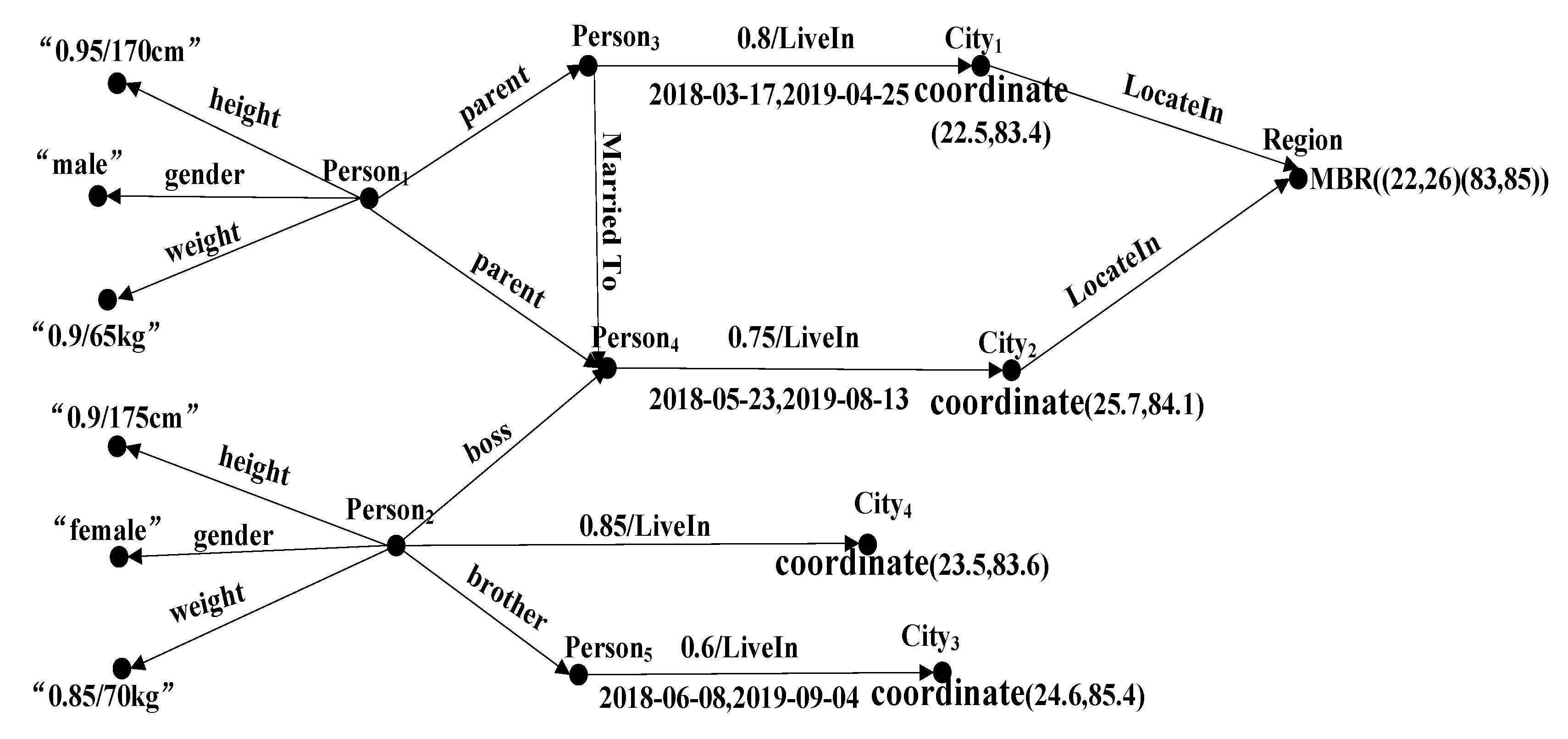
2. Fuzzy Spatiotemporal RDF Data Model

This section firstly proposes a portrayal strategy for fuzzy spatiotemporal RDF information and a fuzzy spatiotemporal RDF diagram model. Secondly, it proposes the basic concepts of a fuzzy spatiotemporal RDF graph, including the subgraph, isomorphism, graph pattern, and graph pattern matching, which lays a foundation for the algebra of a fuzzy spatiotemporal RDF graph in the next section.

An abstract fuzzy spatiotemporal data statement is defined as follows to express fuzzy spatiotemporal data:

Definition 1. 

A fuzzy spatiotemporal statement is a quintuple <μ_s/s, μ_p/p, μ_o/o, L, T>, where s, p, o, L, and T represent subject, predicate, object, location, and time interval, respectively, μs, μ_p, and μ_o represent the fuzzy degree.

The traditional RDF statement, where s, p, and o are the traditional RDF elements, is extended by the fuzzy spatiotemporal statement, but s and o adds the spatial attribute, p adds the temporal attribute, and μ_s, μ_p, and μ_o represent their fuzzy degree, respectively. L designates a subjective or objective spatial feature (the coordinates). To indicate the period time that the assertion is valid, T has the start time T_s and the end time T_e, i.e., the statement is seen as plausible during the time frame; specifically, T_s = T_e if and only if the statement occurs at a specific point in time.

A diagram is the fundamental building block of a fuzzy spatiotemporal RDF information model. Let us first introduce some simple concepts about tuple and graphic conversion. Let V be a limited arrangement of vertices, E ⊂ V_i ’ V_j is a collection of edges. Here are a few cases:

(1)

If V and E are general vertices and edges, respectively, i.e., nonspatial entities and nontemporal statements, then L: V∪E → Σ₁ is the mapping from vertices and edges to Σ₁, a collection of labels called the string;

(2)

If V is a vertex with the spatial attribute, then S: V → Σ₂ is a mapping from vertices to Σ₂, a collection of labels called the coordinate;

(3)

If E is an edge with the temporal attribute, then T: E → Σ₃ is a mapping from edges to Σ₃, a collection of labels called the date.

The abovementioned components of the sextuple G_M = (V, E, Σ, L, S, T) make up a labeled directed graph. Let M be a collection of spatiotemporal RDF quintuples, with each quintuple represented as $\left(s,p,o,L,T\right)\in \left(U\cup B\right)\times \left(U\right)\times \left(U\cup B\cup L\right)\times \left(C\right)\times \left(D\right)$. The following two steps are part of a conversion function from M to G_M for each (s, p, o, L, T) ∊ M:

(1)

Add vertices v_s and v_o to V, assign L_v (v_s) = s and L_v (v_o) = o, and assign S_v (v) = L if the vertex represent a spatial entity;

(2)

Add a directed edge (v_s, v_o) into E, assign L_e (v_s, v_o) = p, and assign T_e (v_s, v_o) = T if the edge has a temporal property.

It ought to be noticed that the chart structure just momentarily depicts the primary qualities of the spatiotemporal RDF information model, disregarding fuzzy items in vertices and edges of the spatiotemporal RDF information model. The following is a more detailed explanation of the formal definition of the fuzzy spatiotemporal RDF chart information model.

Definition 2. 

(Fuzzy spatiotemporal RDF data graph). A nonuple (V, E, Σ, L_v, L_e, S_v, T_e, μ, ρ) represents the fuzzy spatiotemporal RDF data graph G, where

(1) 

V is a limited arrangement of vertices;

(2) 

$E\subset V_i\times V_j$is a collection of coordinated edges between vertices, where$V_i\times V_j\subset V$;

(3) 

Σ = {Σ₁, Σ₂, Σ₃} is a collection of labels, where Σ₁ is a collection of general vertices and edges labels, Σ₂ is a collection of spatial labels of vertices, and the spatial vertices labels indicate the coordinates of the entities (the events), i.e., the latitude and longitude. Σ₃ is a collection of edges with temporal labels, where the labels identify the period time in which the object (the event) happens, i.e., the start time and the end time;

(4) 

L_v: V → Σ₁ is a function that assigns vertices literal labels;

(5) 

L_e: E → Σ₁ is a function that assigns edges literal labels;

(6) 

S_v: V → Σ₂ is a function that assigns vertices spatial labels;

(7) 

T_e: E → Σ₃ is a function that assigns edges temporal labels;

(8) 

μ: V → [0, 1] is a fuzzy subset of vertices;

(9) 

ρ: E → [0, 1] is a fuzzy connection on fuzzy subset μ. Notice that “v_i, v_j ∊ V, ρ(v_i × v_j) ≤ μ(v_i) ∧ μ(v_j), where ∧ represents the minimum value.

Each vertex v_i ∊ V of graph G in Definition 2 has a literal label L_v(v_i), and also includes a spatial label S_v(v_i) for the spatial vertex, relating to the subject or protest in the spatiotemporal RDF dataset. Additionally, the directed edge (v_i, v_j) ∈E is a directed edge from vertex v_i to vertex v_j, which corresponds to the predicate in the fuzzy spatiotemporal statement and has the literal label L_e (v_i, v_j) as well as the temporal label T_e (v_i, v_j) for the temporal edge. The strict name worth of a vertex is related to the fuzzy degree, which shows the chance of the vertex taking the mark, and the fuzzy worth related to each edge tends to the consistency level of the contrasting association between vertices. A fuzzy spatiotemporal RDF data chart could contain both fuzzy vertices (edges) with μ_s and μ_p ∊ (0, 1) and fresh vertices (edges) with μ_s and μ_p = 0, 1.

Example 1. 

An illustration of fuzzy spatiotemporal RDF data is given in

Table 1. Fuzzy spatiotemporal RDF data.

Num	Fuzzy/Subject	Fuzzy/Predict	Fuzzy/Object	Location (x, y)	Start Time	End Time
#1	Person1	Height	0.95/170 cm
#2	Person1	Gender	Male
#3	Person1	Weight	0.9/60 kg
#4	Person1	Parent	Person3
#5	Person1	Parent	Person4
#6	Person2	Height	0.9/175 cm
#7	Person2	0.85/live in	City4	Coordinate (23.5, 83.6)	15 August 2018	17 November 2019
#8	Person2	Gender	Female
#9	Person2	Weight	0.85/70 kg
#10	Person2	Boss	Person4
#11	Person2	Brother	Person5
#12	Person3	Married to	Person4
#13	Person3	0.8/live in	City1	Coordinate (22.5, 83.4)	17 March 2018	25 April 2019
#14	Person4	Live in	City2	Coordinate (25.7, 84.1)	23 May 2018	13 August 2019
#15	Person5	0.8/live in	City3	Coordinate (24.6, 85.4)	9 June 2018	4 September 2019
#16	City1	Located in	Region	MBR ((22, 26) (83, 85))
#17	City2	Located in	Region	MBR ((22, 26) (83, 85))

and the corresponding graph is given in Figure 1. It describes some information about the persons and their relationships. Here, the gender of person1 is male, their height is “170 cm”, their weight is “65 kg”, and the parent is person3, who lived in “city1 coordinate (22.5, 83.4)” from 17 March 2018 to 25 April 2019. As seen from the chart, the level of person1 has a strict mark of “170 cm” with a chance of 0.95, which precisely relates to the triple (person1, height, 0.95/“170 cm”). Essentially, the vertex marked “person3” is associated with another vertex named “city1 coordinate (22.5, 83.4)” through the coordinated edge named “live in” with a chance of 0.8, which relates to the quintuple (person3, 0.8/live in, “city1”, “coordinate (22.5, 83.4)”, “17 March 2018, 25 April 2019”). Hence, this realistic portrayal was sufficiently nonexclusive to catch the relationships or limitations among the labels of vertices and edges.

Definition 3. 

(Fuzzy spatiotemporal RDF subgraph). A fuzzy spatiotemporal RDF graph$G^{\prime }= (V^{\prime },E^{\prime },{\Sigma }^{\prime },L^{\prime },S^{\prime },T^{\prime },{\mu }^{\prime },{\rho }^{\prime })$is known as a fractional fuzzy spatiotemporal subchart of$G= \left(V,E,\Sigma ,L,S,T,\mu ,\rho \right)$if

(1)

${\mu }^{\prime }\subseteq \mu ,{\rho }^{\prime }\subseteq \rho ,V^{\prime }\subseteq V,E^{\prime }\subseteq E$and${\Sigma }^{\prime }\subseteq \Sigma$;

(2)

$\forall u\in V^{\prime },{\mu }^{\prime }\left(u\right)\le \mu \left(u\right)$;

(3)

$\forall \left(u,v\right)\in E^{\prime },{\rho }^{\prime }\left(u,v\right)\le \rho \left(u,v\right)$.

Particularly, a halfway fuzzy spatiotemporal subgraph G′ is known as a fuzzy spatiotemporal subgraph of G, if

(1)

$\forall u\in \{x\in V^{\prime }:{\mu }^{\prime }\left(x\right) > 0\},{\mu }^{\prime }\left(u\right) =\mu \left(u\right)$ and

(2)

$\forall \left(u,v\right)\in \{\left(x,y\right)\in V^{\prime }\times V^{\prime }:{\rho }^{\prime }\left(x,y\right) > 0\},{\rho }^{\prime }\left(u,v\right) =\rho \left(u,v\right)$, which is written as G′ ⊆ G.

Definition 4. 

(Fuzzy spatiotemporal RDF graph isomorphism). Given the two fuzzy spatiotemporal RDF graphs G₁ = (V₁, E₁, Σ₁, L₁, S₁, T₁, μ₁, ρ₁) and G₂ = (V₂, E₂, Σ₂, L₂, S₂, T₂, μ₂, ρ₂), in case there is a bijective function h: V₁ → V₂ satisfy:

(1) 

$\forall u\in V_1,h\left(u\right)\in V_2,L_1\left(u\right)= L_2\left(h\left(u\right)\right)$,$S_1\left(u\right)= S_2\left(h\left(u\right)\right)$and${\mu }_1\left(u\right)= {\mu }_2\left(h\left(u\right)\right)$;

(2) 

$\forall \left(u,v\right)\in E_1$,$\left(h\left(u\right),h\left(v\right)\right)\in E_2$,$L_1\left(u,v\right)= L_2\left(h\left(u\right),h\left(v\right)\right)$,$T_1\left(u,v\right)= T_2\left(h\left(u\right),h\left(v\right)\right)$,${\rho }_1\left(u,v\right)= {\rho }_2\left(h\left(u\right),h\left(v\right)\right)$, then G₁ is isomorphic to G₂, which is denoted as G₁≅G₂.

Given the two fuzzy spatiotemporal RDF graphs Q and G, if Q is homogeneous on subgraph G′ of G, and G′ is a match of Q in G, then Q is an isomorphic subgraph to G, which is indicated as Q ⊆ G.

Definition 5. 

(Fuzzy spatiotemporal RDF graph pattern). A fuzzy spatiotemporal RDF graph pattern is a septuple P = (V_P, E_P, F_V, S_V, F_E, T_E, R_E) where

(1) 

V_P is a finite set of vertexes.

(2) 

E_P is a finite set of directed edges.

(3) 

F_V and S_V are functions defined on V_P. For a given vertex u ∊V_P, F_V (u) is the predicate applied to the literal label worth of vertex u. Similarly, S_V (u) is the predicate applied to the spatial mark worth of vertex u. These predicates are a Boolean mix of the nuclear predicate, each predicate looks at a steady c determined in the example with the worth V_i using a given operator θ$(e.g.<,\le ,=,>,\ge ,\ne )$. Let c_j be a consistent and θ_j be a correlation administrator, F_V (u) ∨ S_V (u) are the mix of nuclear predicates of the structure (V_iθ_jc_j) by the intelligent connectives (∧,∨,¬).

(4) 

F_E and S_E are functions defined on E_P, which are the counterpart of F_V and S_V for edges.

(5) 

R_E: E_P→ re (E) is a capability characterized by E_P. For each (u, v) in E_P, re (E) is a way of normal articulation, where E is a set that is comprised of the data graph G, variables and wildcard *, which can be developed as R::= e|R₁·R₂|R₁|R₂|R⁺. Here, e denotes the edge labeled by e or wildcard symbol matching any label in Σ, R₁·R₂ denotes the concatenation of expressions, R₁|R₂ denotes disjunction of expressions, and R⁺ denotes one or more occurrences of R.

Example 2. 

Figure 2 shows the graph pattern P of the fuzzy spatiotemporal RDF graph shown in Figure 1. This pattern concerns the person (? pb) who lives in city (? C), whose children (? pa) weigh more than 60 kg (? w > 60 kg), and whose gender is male.

We can see that chart design P indicates the topological and content-based requirements picked by the client. Then, we present the thought of a fuzzy spatiotemporal RDF chart design matching which sums up the subdiagram isomorphism. Naturally talking, given a fuzzy spatiotemporal RDF information chart G, the semantics of a diagram design P characterizes a bunch of matches, in which each match matches the example to an isomorphic subchart of G.

Definition 6. 

(Fuzzy spatiotemporal RDF graph pattern matching). A fuzzy spatiotemporal RDF graph pattern P = (V_P, E_P, F_V, S_V, F_E, T_E, R_E) is coordinating with a fuzzy spatiotemporal RDF data graph G = (V, E, Σ, L, S, T, μ, ρ) with a fulfillment degree δ_P (G), assuming that there is an injective planning φ: P → G which is all-out planning from vertexes and edges of P to vertexes and ways of G to such an extent that:

(1) 

(Matching vertex) each vertex on V_P has a picture vertex on V by the injective capability. Officially, for every vertex u ∈, there is a vertex φ (u) ∈V, associated with a satisfactory degree${\delta }_u(V)=\mu \left(\phi \left(u\right)\right)$.

(2) 

(Matching edge) φ jelly the chart construction of P. For each edge (u, v) ∈ E_P, there are two vertices φ (u) and φ (v) of V s.t. There is a path p in G from φ (u) to φ (v) s.t. ρ coordinates standard articulation re with a fulfillment degree, δ_re (p), characterized as follows, as indicated by the type of re (in the accompanying, R, R₁, and R₂ are standard articulations):

• If re is an edge labeled by e or a wildcard symbol *, and if p is an edge e′ from vertex φ (u) to φ (v), where then else$e^{\prime }=e(e^{\prime }\in E)$then${\delta }_{re}\left(p\right)=\rho \left(\phi \left(u\right),\phi \left(v\right)\right)$else${\delta }_{re}\left(p\right)=0$.
• If re is of the form R₁ · R₂, and P is the set of all pairs of paths (p₁, p₂) s.t. p is of the form p₁p₂, then${\delta }_{re}\left(p\right)=\max p\left(min \left({\delta }_R{}_1(p_1),{\delta }_R{}_2\left(p_2\right)\right)\right)$.
• If re is of the form R₁|R₂ then δ_re (p) = max (δ_R1 (p), δ_R2 (p)).
• If re is of the form R⁺, and P is the set of all tuples of paths (p₁,…,p_n) (n > 0) s.t. p is of the form p₁ ···p_n. One has δ_re(p) = max_P (min(δ_R (p₁), …, δ_R1 (p_n))).

(3) 

(Checking conditions on the vertex and edge label) the condition (or predicate) of vertex and edge of P is matched with G. Formally, L(φ(u)) satisfies the formula F_V, S(φ(u)) satisfies the formula S_V for all u∊ V_P, L (φ(u), φ(v)) satisfies the formula F_E, T (φ(u), φ(v)) satisfies the formula F_E for all (u, v) ∊ E_P. If the condition is assessed to be valid, the fulfillment degree is 1, otherwise 0.

(4) 

The worth of δ_P (G) is the base worth of the fulfillment degrees coming about because of the matches and conditions in (1), (2), and (3). If there is no match, then δ_P (G) = 0, i.e., G does not match P.

3. Graph Algebra for Fuzzy Spatiotemporal RDF

The mathematical methodology is a viable way to query data set frameworks. In the meantime, variable-based math activities can be likewise applied in SPARQL. In this segment, we think about several conventional variable-based math activities for SPARQL diagram design, for instance union, selection, left join, and projection, in light of the fact that these operations could be straightforwardly applied in the Union, Filter, Optional, and Select expressions of SPARQL, separately. Furthermore, we likewise add extra operations to manage the fuzzy spatiotemporal RDF chart model. We plan our variable-based math which can be gathered into three essential arrangements of operations: chart set activities, design matching operations, and development operations. The diagram set operations take an assortment of charts and perform set-hypothetical activities. The pattern-matching operations are situated to primary determination and extraction. The development activities are intended to work with the development of the fuzzy spatiotemporal RDF query graph by making and embedding new vertices/edges and controlling the extricated structures.

3.1. Set Operations

Set operations carry out set-theoretical operations after taking a collection of diagrams as input. There are four different types of common fuzzy spatiotemporal set-diagram operations listed here: union (∪), intersection (∩), Cartesian product (×), and difference (−).

Definition 7. 

(Fuzzy spatiotemporal union). Give G₁ = (V₁, E₁, Σ₁, L₁, S₁, T₁, μ₁, ρ₁) and G₂ = (V₂, E₂, Σ₂, L₂, S₂, T₂, μ₂, ρ₂) each a pair of fuzzy spatiotemporal RDF subgraphs of G, respectively. The following describes the fuzzy spatiotemporal union of G₁ and G₂.

G₁∪G₂ = (V_r, E_r, Σ_r, L_r, S_r, T_r, μ_r, ρ_r)

In the standard set theory union, where V_r = V₁∪V₂, E_r = E₁∪E₂, Σ_r = Σ₁∪Σ₂, L_r = L₁∪L₂, S_r = S₁ ∪S₂, and T_r = T₁∪T₂ [25], μ_r and ρ_r are the participation level of the fuzzy spatiotemporal association result, separately. Here,

$$\begin{array}{l}{\mu }_r(v)=\left\{\begin{array}{cc}{\mu }_1(v),& \forall v\in V_1-V_2\\ {\mu }_2(v),& \forall v\in V_2-V_1\\ {\mu }_1(v)\vee {\mu }_2(v),& \forall v\in V_1\cap V_2\end{array}\right.\\ \end{array}$$

$$\begin{array}{l}\rho r(vi,vj)=\left\{\begin{array}{cc}\rho 1(v_i,v_j),& \forall (v_i,v_j)\in E_1-E_2\\ \rho 2(v_i,v_j),& \forall (v_i,v_j)\in E_2-E_1\\ \rho 1(v_i,v_j)\vee {\rho }_2(vi,vj),& \forall (v_i,v_j)\in E_1\cap E_2\end{array}\right.\\ \end{array}$$

and a∨b indicates the highest value of a and b (i.e., a∨b = max (a, b)).

Example 3. 

The fuzzy spatiotemporal RDF charts are shown in Figure 1 and Figure 3a are applied to the fuzzy spatiotemporal association activity. Then, we obtained the aftereffect of the association activity which is displayed in Figure 3b.

Definition 8. 

(Fuzzy spatiotemporal intersection). Give G₁ = (V₁, E₁, Σ₁, L₁, S₁, T₁, μ₁, ρ₁) and G₂ = (V₂, E₂, Σ₂, L₂, S₂, T₂, μ₂, ρ₂) each a pair of fuzzy spatiotemporal RDF subgraphs of G, respectively. The following describes the fuzzy spatiotemporal intersection of G₁ and G₂.

G₁∩G₂ = (V_r, E_r, Σ_r, L_r, S_r, T_r, μ_r, ρ_r)

where V_r = V₁∩V₂, E_r = E₁∩E₂, Σ_r = Σ₁∩Σ₂, L_r = L₁∩L₂, S_r = S₁∩S₂, and T_r, = T₁∩T₂ are the classic set theoretical intersection [25], μ_r(v)= μ₁(v) ∧μ₂(v), “v ∊ V₁∩V₂ and ρ_r(v_i,v_j) = ρ₁(v_i,v_j) ∧ ρ₂(v_i, v_j),”(v_i, v_j) ∊ E₁∩E₂ are the participation level of fuzzy spatiotemporal convergence result, separately, and a∧b denotes the minimum value of a and b, i.e., a∧b = min(a, b).

Example 4. 

The fuzzy spatiotemporal RDF diagrams in Figure 1 and Figure 3a are applied to the fuzzy spatiotemporal crossing point activity. Then, at that point, we come to the aftereffect of the convergence activity displayed in Figure 4.

Definition 9. 

(Fuzzy spatiotemporal Cartesian product). Give G₁ = (V₁, E₁, Σ₁, L₁, S₁, T₁, μ₁, ρ₁) and G₂ = (V₂, E₂, Σ₂, L₂, S₂, T₂, μ₂, ρ₂) each a pair of fuzzy spatiotemporal RDF subgraphs of G, respectively. The following describes the fuzzy spatiotemporal Cartesian product of G₁ and G₂.

G₁ × G₂ = (V_r, E_r, Σ_r, L_r, S_r, T_r, μ_r, ρ_r)

where V_r = V₁×V₂, E_r = {(u, u₂)(u, v₂) | u∊V₁, u₂v₂∊E₂}∪{(u₁,w)(v₁,w)|w∊V₂, u₁v₁∊E₁},μ_r(u₁, u₂) = (μ₁×μ₂)(u₁, u₂) = μ₁(u₁)∧μ₂(u₂),” (u₁, u₂)∊V, and

If ∀u∊V₁, ∀u₂v₂ ∊E₂, then ρ_r = ρ₁ρ₂(u, u₂) (u, u₂) = μ₁ (u)∧ρ₂(u₂v₂)

If∀w∊V₂, ∀u₁v₁ ∊E₁, then ρ_r = ρ₂ (u₁, w) (u₁, w) = μ₂(w)∧ρ₁ (u₁v₁).

As defined above, the edge between the two vertices u and v is connoted by uv as opposed to (u, v), considering the way that in the Cartesian result of two outlines, one vertex of the actual chart is an organized pair.

Example 5. 

Figure 5a,b show two straightforward fuzzy spatiotemporal Cartesian products, and Figure 5c shows the outcome of the fuzzy spatiotemporal G and G′ Cartesian products.

Definition 10. 

(Fuzzy spatiotemporal difference). Give G₁ = (V₁, E₁, Σ₁, L₁, S₁, T₁, μ₁, ρ₁) and G₂ = (V₂, E₂, Σ₂, L₂, S₂, T₂, μ₂, ρ₂) each a pair of fuzzy spatiotemporal RDF subgraphs of G, respectively. The following describes the fuzzy spatiotemporal difference between G₁ and G₂.

G₁ − G₂ = (V_r, E_r, Σ_r, L_r, S_r, T_r, μ_r, ρ_r)

where E_r = E₁ − E₂ is the classic set theoretical difference [25], V_r consists of vertices that are brought about a group of edges in E_r, μ_r (v) = μ₁(v), “v ∊ V_r and ρ_r(v_i, v_j) =ρ₁(v_i, v_j), “(v_i,v_j) ∊E₁ − E₂. Actually, by separating the edges of G₂ from the edges of G₁, the fuzzy spatiotemporal difference between G₁ and G₂ defines a new fuzzy spatiotemporal RDF graph. Notice that G₁ − G₂ is different from G₂ − G₁.

Example 6. 

The output of the fuzzy difference operation G₁ − G₂ is shown in Figure 6, that the fuzzy spatiotemporal RDF graph which is in Figure 1 is represented by graph G1, and the fuzzy spatiotemporal RDF graph which is in Figure 3a is represented by graph G₂.

3.2. Fuzzy Spatiotemporal Selection Operation

By using a chart layout, the fuzzy spatiotemporal selection operation can filter the fuzzy spatiotemporal diagrams. It acknowledges a bunch of fuzzy spatiotemporal diagrams and a fuzzy spatiotemporal chart design as information. The result is a fuzzy spatiotemporal set comprised of all subdiagrams that match the given chart design, which is not just the substance of the right outcome, but also the construction of the goal charts.

Definition 11. 

(Fuzzy spatiotemporal selection). Assume that the fuzzy spatiotemporal RDF data graph G = (V, E, Σ, L, S, T, μ, ρ) exists. The following defines fuzzy spatiotemporal choice for a given fuzzy spatiotemporal RDF network pattern P = (V_P, E_P, F_V, S_V, F_E, T_E, R_E).

$$\sigma p\left(G\right)=\{<g,{\delta }_P\left(g\right)>|g=f\left(P,G\right),{\delta }_P\left(g\right)>0\}$$

where g is a subgraph of G, pattern P and fuzzy spatiotemporal RDF graph G are matched using function f (P, G), and the satisfaction level is measured by δp (g). In the event of copies (the same graph that displays different satisfaction levels), the most noteworthy fulfillment degree is held.

Example 7. 

The result of σp (G) is shown in Figure 7, where G is the fuzzy spatiotemporal data graph in Figure 1 and P is the pattern of the fuzzy spatiotemporal RDF graph used in Example 2. Based on the graph, the person labeled person1 weighs more than 60 kg and his gender is male, person3 and person4 are the parents of person1, and they locate in Region. Furthermore, the regular phrase R_E = “live in. Locate In” is satisfied by the path leading from person3/person4 to Region. In order to match the graph pattern P in the fuzzy spatiotemporal data graph G, there are two solutions (Figure 7a,b). Given that Definition 3 minimum value for fulfillment degrees is the satisfaction degree, we have δ_p (g₁) = 0.8 in Figure 7a and δ_p (g₂) =0.75 in Figure 7b, respectively. Therefore, the final answer is Figure 7b.

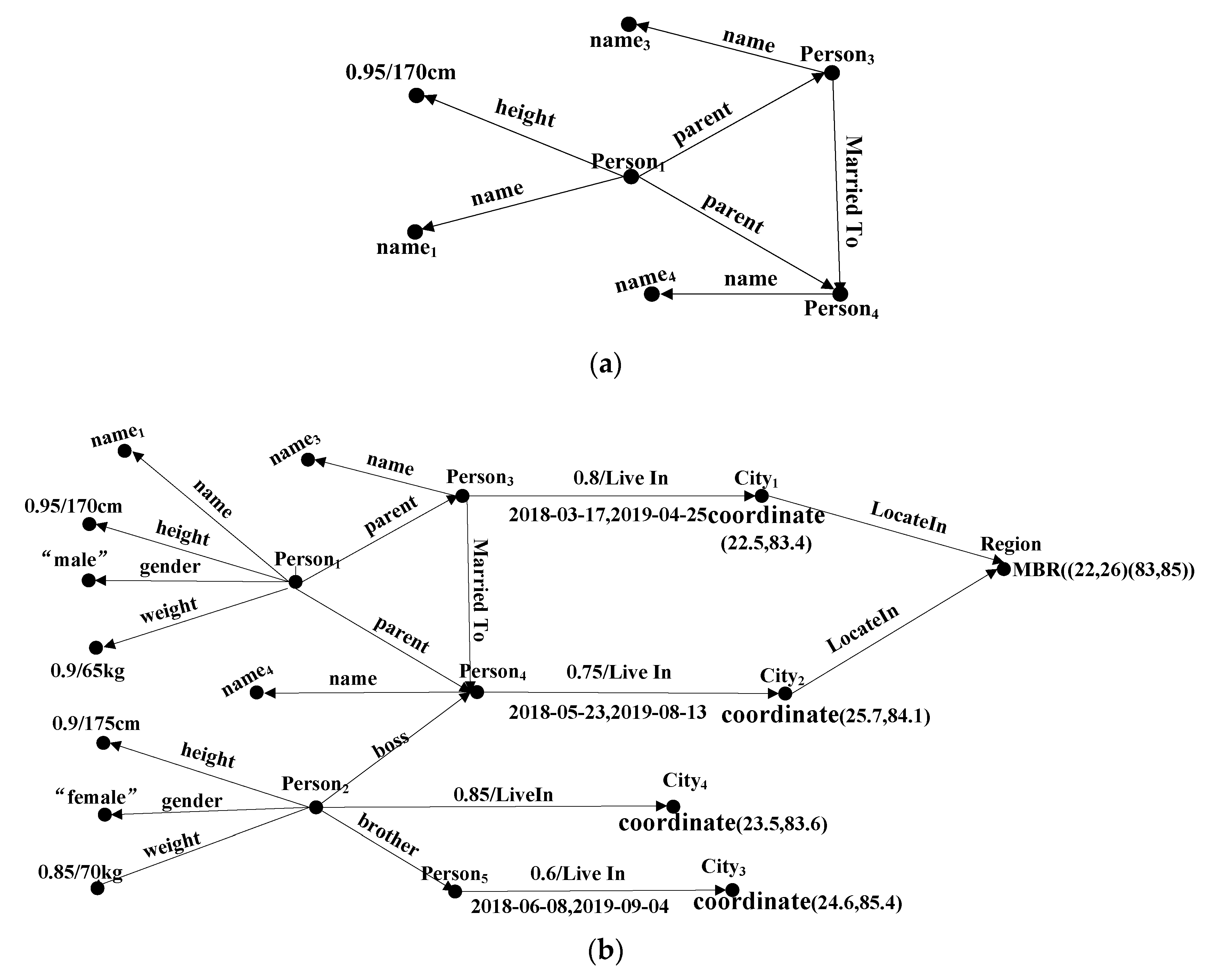
3.3. Fuzzy Spatiotemporal Projection Operation

The fuzzy spatiotemporal projection activity accepts the fuzzy spatiotemporal chart as the info, a spatiotemporal RDF diagram design P, and a projection list PL as the boundaries. The projection list is a list of the names of the objects (vertices and edges) that appear in example P. The projection’s output includes every article that appears in the P, and the various leveled relationship among the items in the first information format for a chart is safeguarded.

Notice that, if this projection list is empty, only the matching images are returned. This implies that other things besides those predefined in the fuzzy spatiotemporal RDF information diagram may be disposed of by the fuzzy spatiotemporal projection. The projection action is described in the manner below.

Definition 12. 

(Fuzzy spatiotemporal projection). Allow G = (V, E, Σ, L, S, T, μ, ρ) to be a fuzzy spatiotemporal RDF information chart, ϖ is a fuzzy spatiotemporal projection capability and P is a fuzzy spatiotemporal RDF diagram design. Then, at that point, the fuzzy spatiotemporal projection can be characterized as follows.

$${\pi }_{P,PL}\left(G\right)=\{<g,{\delta }_T\left(g\right)>|g=\varpi \left(P,PL,G\right),{\delta }_T\left(g\right)>0\}$$

The result of the projection action is a fuzzy spatiotemporal plan of diagrams, and δ_T (g) is the satisfaction degree. The fuzzy spatiotemporal projection action returns a fuzzy spatiotemporal set, which comprises all suboutlines of G that match the fuzzy spatiotemporal chart plan P.

Example 8. 

We apply a similar example diagram of Figure 2 and a projection activity to the fuzzy spatiotemporal RDF chart of Figure 1. Then we obtain the aftereffect of the projection activity as displayed in Figure 8. The fulfillment degree δ_T (g) is 0.75. There are clear differentiations between the outcome plans of assurance and projection activities.

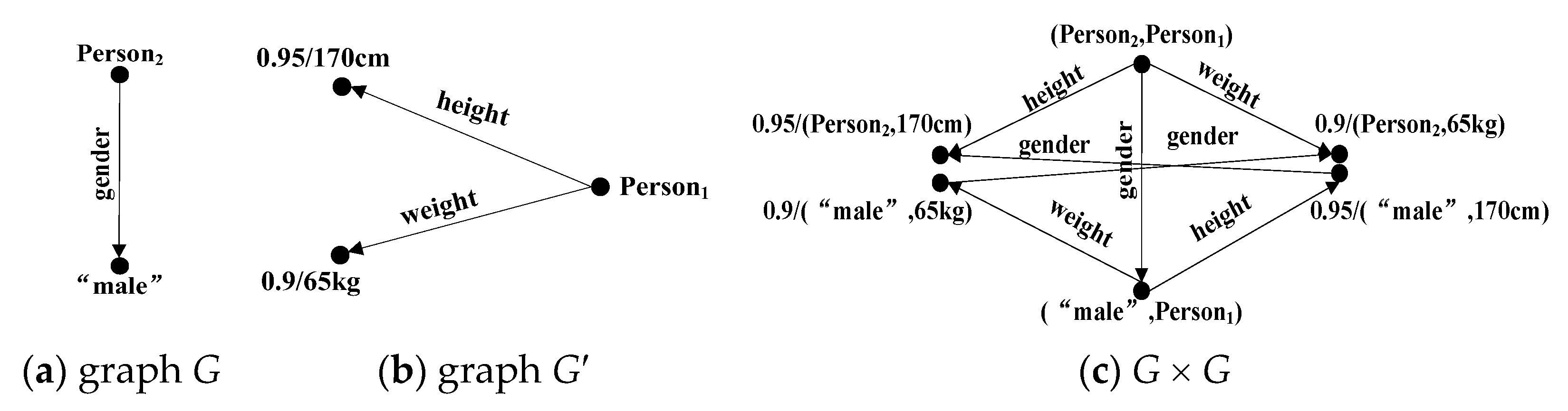
3.4. Fuzzy Spatiotemporal Join Operation

Information diagrams are joined by the fuzzy spatiotemporal join activity using an example. Join can be expressed as a Cartesian item followed by a fuzzy spatiotemporal determination, just like in social variable-based math. The state of choice is to think about the characteristic of the main diagram with another chart. In a regarded join, the join condition is a predicate on vertex names. In an essential join, the constituent charts can be associated with edges.

Definition 13. 

(Fuzzy spatiotemporal join). Allow G₁ and G₂ to be two fuzzy spatiotemporal RDF diagrams and P to be a fuzzy spatiotemporal RDF chart design. Then, at that point, the fuzzy spatiotemporal joint activity is characterized as follows.

$$G_1\bowtie p{G}_2 = \{g |g =op (G_1 \times G_2)\}$$

where P is to be matched against (G₁ × G₂), and somewhere around one predicate f in the Fv ∨ S_v of P is L (v₁) = L (v₂) and S (v₁) = S (v₂), here v₁ matches vertices in G₁, and v₂ matches vertices in G₂. That is, L (v₁) alludes to a vertex exacting mark in G₁ and L (v₂) to one in G₂. S (v₁) alludes to a vertex spatial name in G₁ and L (v₂) to one in G₂.

The left join of the above articulations is meant as G₁⋊pG₂, which has the following semantics: P₁ and P₂ are the two sections in P that are matched against G₁ and G₂ separately, assuming that the matching diagram G′₂ obtained from σp₂ (G₂) does not satisfy the join condition L (v₁) = L (v₂) and S (v₁) = S (v₂), then output just σp₁ (G₁); otherwise, output σ_p (G₁ × G₂).

3.5. Construction Operations

Querying a fuzzy spatiotemporal RDF diagram not only suggests separating fascinating substances from the info model, yet additionally developing a result model by implanting new vertices/edges or by eradicating vertices/edges from the eliminated outline. The development operations are intended to work with the development of fuzzy spatiotemporal RDF inquiries result chart.

3.5.1. Vertex Deletion

The vertex erasure activity eliminates the distinguished vertices from a diagram. An erase determination is utilized to recognize vertices, and it demonstrates which vertices to erase by the vertex label.

Definition 14. 

(Vertex deletion). Officially, the erase activity takes a fuzzy spatiotemporal information diagram G = (V, E, Σ, L, S, T, μ, ρ) as the info and an erase detail DS as the boundary. The erase determination is a gathering of vertices names showing up in G. DS ⊂ {Σ₁, Σ₂}, where the Σ₁, Σ₂ represent literal labels and spatial labels, respectively. It produces a fuzzy spatiotemporal diagram characterized as follows:

$$K \left(G, DS\right)=\left\{g\hspace{0.17em}|\hspace{0.17em}g\hspace{0.17em}=\hspace{0.17em}\left(V^{\prime }, E^{\prime }, \mathsf{\Sigma }, L, S, T, \mu , \rho \right)\right\}$$

where$V^{\prime }=\{v\hspace{0.17em}|\hspace{0.17em}v\in V\hspace{0.17em}and\hspace{0.17em}{L}_v\left(v\right)\notin {\mathsf{\Sigma }}_1,S_v\left(v\right)\notin {\mathsf{\Sigma }}_2\}$and E′ is the limitation of E over V′ × V′.

Note that vertex cancellation is the same as projection. As a matter of fact, it tends to be viewed as a corresponding activity with projection, indicating the vertices to be disposed of as opposed to vertices to be held.

3.5.2. Edge Deletion

The idea behind edge erasure and vertex cancellation are similar. The relationships from a fuzzy spatiotemporal RDF chart are eliminated.

Definition 15. 

(Edge deletion). Edge erasure activity takes a fuzzy spatiotemporal diagram G, and a gathering of edge names ES as the input, ES ⊂{Σ₁, Σ₃}, where the Σ₁, Σ₃ address exacting names and fleeting marks, separately. It produces a fuzzy spatiotemporal chart with the following attributes:

$$\lambda \left(G,ES\right)=\{g\hspace{0.17em}|\hspace{0.17em}g=(V,E^{\prime },\mathsf{\Sigma },L,S,T,\mu ,\rho )\}$$

Here,$E^{\prime }=\{e\hspace{0.17em}|\hspace{0.17em}e\in E\hspace{0.17em}and\hspace{0.17em}{L}_e\left(e\right)\notin {\mathsf{\Sigma }}_1,T_e\left(e\right)\notin {\mathsf{\Sigma }}_3\}$.

3.5.3. Vertex Insertion

The fuzzy spatiotemporal RDF information chart may obtain another vertex as a result of the vertex inclusion action. The sort of the new vertex is an asset, clear, strict, or spatial element, on the off chance that the vertex addresses an asset, the name of the new vertex is a URIs; on the off chance that the vertex addresses a strict, the name of the new vertex is a string; assuming the vertex addresses a spatial substance, the mark of the new vertex is a direction.

Definition 16. 

(Vertex insertion). Allow G to be a fuzzy spatiotemporal RDF diagram, IS to be a supplement detail which is a bunch of vertices names, and δ to be the fuzzy level of the supplement vertex. The vertex inclusion activity returns a fuzzy spatiotemporal diagram including the embedded vertices.

$$\Phi \left(G,IS\right)=\{g\hspace{0.17em}|\hspace{0.17em}g=(V^{\prime },E,{\mathsf{\Sigma }}^{\prime },L,S,T,\mu ,\rho )\}$$

Here,$V^{\prime }=V\cup \{v^{\prime }\hspace{0.17em}|\hspace{0.17em}L(v^{\prime })\in IS\hspace{0.17em}\mathrm{and}\hspace{0.17em}\mu (v^{\prime }) =\delta \}\hspace{0.17em}\mathrm{and}\hspace{0.17em}{\mathsf{\Sigma }}^{\prime }=\mathsf{\Sigma }\cup IS$.

3.5.4. Edge Insertion

The spatiotemporal RDF information diagram’s edge inclusion action adds a new valid or temporary edge to link the subject and item.

Definition 17. 

(Edge insertion). Allow G to be a fuzzy spatiotemporal RDF diagram, EI be the edges names, EI ⊂ {Σ₁, Σ₃}, where the Σ₁, Σ₃ represent literal labels and temporal labels, respectively. Δ be a fuzzy level of the addition edges. The activity that includes edges produces a fuzzy spatiotemporal diagram that contains the embedded edges.

$$\mathsf{\Phi }\left(G,ES\right)=\{g\hspace{0.17em}|\hspace{0.17em}g=(V,E^{\prime },{\mathsf{\Sigma }}^{\prime },L,S,T,\mu ,\rho )\}$$

Here,$E^{\prime }=E\cup \{e^{\prime }\hspace{0.17em}|\hspace{0.17em}L(e^{\prime })\in EI\hspace{0.17em}\mathrm{and}\hspace{0.17em}\rho (e^{\prime })=\delta \}\hspace{0.17em}\mathrm{and}\hspace{0.17em}{\mathsf{\Sigma }}^{\prime }=\mathsf{\Sigma }\cup EI$.

4. Relationship of SPARQL Queries and the Fuzzy Spatiotemporal RDF Algebraic Operations

Displaying fuzzy spatiotemporal RDF alone is insufficient to meet the challenges of practical application; fuzzy spatiotemporal RDF querying is exceptionally fundamental. In this segment the qualities of SPARQL, first and foremost the query language in a fuzzy spatiotemporal RDF, are depicted, and afterward, the change from the SPARQL question to a comparable RDF logarithmic expression is explained.

4.1. SPARQL Query in the Fuzzy Spatiotemporal RDF

Classical SPARQL queries lack flexibility and can only query non-spatiotemporal and crisp RDF. We expand the SPARQL to query fuzzy spatiotemporal RDF. The extended SPARQL queries we consider follow the arrangement:

Select [projection clause]

From [graph]

Where [graph pattern]

Channel [condition]

[With<threshold>]

The overall structure of the extended SPARQL is represented by the keywords Select, From, Where, Filter, and With.

(1)

The keyword Select contains a range of factors that are launched from the fuzzy spatiotemporal RDF information base. SPARQL permits a few types of information to be returned: a table using Select, a chart utilizing Depict or Construct, or a True/False response utilizing Ask.

(2)

The watchword indicates the informational collection of a de-issue chart and at least zero named diagrams to question.

(3)

The catchphrase Where provision comprises multituple designs as s p o (L T).

(4)

The keywords Filter condition contains at least one spatiotemporal predicates. We only take into account WITHIN predicates (for spatial choices), DISTANCE predicates (for spatial joins), and TIME predicates (for temporal choices) in our discourse and models for simplicity’s sake.

(5)

The keywords with address the condition should be fulfilled as the base participation degree edge in [0, 1]. Clients pick a proper worth to communicate his/her prerequisite.

Using such SPARQL, one can find solutions that fulfill the given spatiotemporal question condition and the given limit. In this manner, contingent upon the various limits in [0, 1], a similar query for the equivalent fuzzy spatiotemporal RDF might have unique inquiry responses. The query of fuzzy spatiotemporal RDF data sets includes an enormous number of decisions of the edge. Note that the thing With <threshold> can be discarded. The default of <threshold> is exactly one right now.

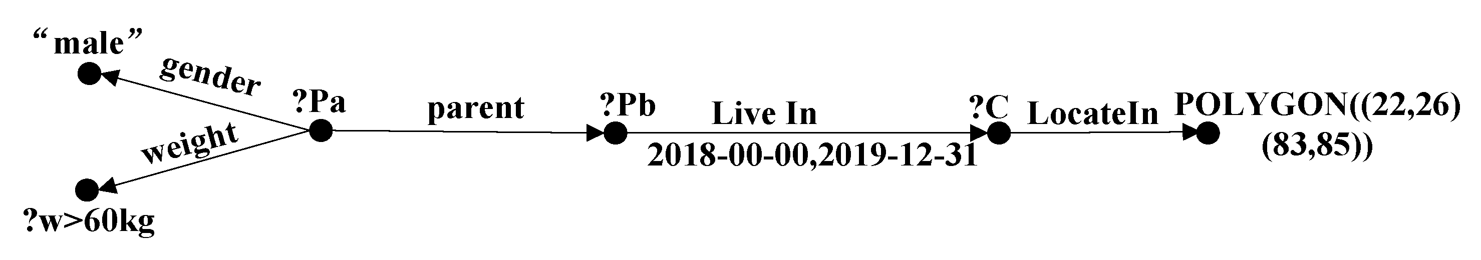
4.2. Translating SPARQL Query Pattern into Fuzzy Spatiotemporal RDF Algebraic Formalism

The main inspiration for planning the fuzzy spatiotemporal RDF diagram model is to involve it as the reason for the effective execution of fuzzy spatiotemporal RDF inquiry language. As the standard inquiry language for the RDF, SPARQL permits us to fabricate complex gathering diagram designs. Bunch examples can be utilized to limit the extent of inquiry conditions to specific pieces of the example. Additionally, it is feasible to characterize subdesigns as discretionary or give various elective examples. In this segment, we start with the expressive force of fuzzy spatiotemporal RDF variable-based math, which is the centerpiece of SPARQL question dialects. Then, at that point, we show that each SPARQL query example could be converted into our fuzzy spatiotemporal RDF mathematical wording introduced above, and give the technique to play out this interpretation.

Our fuzzy spatiotemporal RDF polynomial math is demarked because of the expressive capacity of SPARQL. The SPARQL design articulations from where the condition can undoubtedly be converted into fuzzy spatiotemporal RDF arithmetical articulations. On the other hand, interpretation isn’t generally doable on the grounds that there are fuzzy spatiotemporal RDF variable-based math articulations (e.g., expressions with construction operations) that can’t be communicated in SPARQL. Prior to giving the system to play out this change, we talk about the change rules of the SPARQL design into fuzzy spatiotemporal RDF variable-based math articulation. We don’t audit the total surface punctuation of SPARQL, yet, essentially present the basic mathematical activities utilizing our documentation. Allow G to be a fuzzy spatiotemporal RDF chart over a RDF dataset D, t indicates a tuple pattern, P, P₁, and P₂ be basic SPARQL chart examples, R a channel condition, and S a bunch of factors.

Table 2. The translation rules of a SPARQL query pattern into fuzzy spatiotemporal RDF graph algebra expressions.

Original SPARQL Syntax	Algebraic Syntax
$\left\{t\right\}$	$\left(t\right)$
$\left\{P_1\right\}Optional\left\{P_2\right\}$	$P_1⋊P_2$
$\left\{P_1\right\}Union\left\{P_2\right\}$	$\begin{array}{l}{P}_1\cup P_2\hfill \end{array}$
$\left\{P_1.P_2\right\}$	P1 ⋈ P2
$\left\{PFilterR\right\}$	${\sigma }_R\left(P\right)$

gives the interpretation rules of the SPARQL inquiry mode and fuzzy spatiotemporal RDF variable-based math.

A SPARQL inquiry design is an essential chart example or gathering diagram design, which comprises the tuple blocks, Filter, Optional, and Union chart plan. Some of which contain other diagram designs. The above interpretation is applied to a solitary SPARQL bunch diagram design. Settled bunch diagram design blocks in the Where clauses additionally can be effortlessly dealt with.

In addition to such a change in rules, it is additionally important to characterize how to change SPARQL questions into articulations of the polynomial math. In light of the above interpretation of the rules, we can change any SPARQL designs into variable-based math articulation. For clarity reasons, we expect that the interpretation of tuple blocks is given. In Algorithm 1, we show the change capability Translate (G).

Algorithm 1.

Input: a SPARQL pattern G

Output: an algebraic expression A

1: A = φ; F = φ

2: for each syntactic form g in G do

3:   if g is triple pattern t then

4:     A = (A ⋈ (t))

5:   if g is Optional {P} then

6:     A = (A ⋊ Translate (P))

7:   if g is {P1} Union…Union {Pn} then

8:     if n > 1 then

9:        A′ = (Translate (P1)∪…∪Translate (Pn))

10:    else

11:       A′ = Translate (P1)

12:    A = (A⋈A′)

13:   if g is Filter{R} then

14:     F = F∧{R}

15: end for

16: if F ≠ φ then

17:  A = σF (A)

Algorithm 1 comprises three stages. In the primary stage (Lines 1), the sets A and F are at first vacant, where the example and separating conditions are put away separately; in the subsequent stage (Lines 2–15), the interpretation is performed to obtain all the mathematical articulation of g in a bunch diagram design G. For each understanding circle, if subplan g is a tuple plan or tuple block, joint action is preshaped to accumulate tuples and blocks (Line 3–4). Then, for each subplan g with Optional, a left join action is per-shaped to give optional organizing (Lines 5–6). Then, at that point, all occasions of the Union are imparted using the twofold executive affiliation (Lines 7–12). At last, in the event that g is an administrator Filter, and R is a SPARQL underlying condition, a combination administrator is performed to join channel conditions R and F as essential imperatives (Lines 13–14). This framework is repeated until all subplans in G have been translated. In the event that F isn’t vacant, consolidate it with A in the choice administrator of fuzzy spatiotemporal RDF variable-based math operations (Lines 16–17).

Algorithm 1 centers around the center section of the SPARQL question design, consequently forcing the accompanying limitations on diagram designs and the interpretation cycle. The calculation, most importantly, will be centered around the method of performing SPARQL design interpretation no matter what the arrangement modifiers and the result of a SPARQL inquiry. Second, clear vertices are not thought of. This improvement is forced to focus on the example matching piece of the language. Thirdly, the set semantics of diagram designs are examined.

In the following, we tell the best way to utilize fuzzy spatiotemporal RDF arithmetical articulation to address a SPARQL query. For comfort, we utilize regular language straight away to communicate the fuzzy spatiotemporal RDF questions. Then, at that point, we furnish the SPARQL question explanation alongside their identical RDF mathematical articulation.

Example 9. 

Assume we will inquire about the name of an individual and his/her parent’s name. The person weighs over 60 kg. During 2018.01.01 to 2019.12.31, his/her parent’s lived in “MBR ((22, 26) (83, 85))” and less than 10 km from the coordinate (24, 84), and optionally (i.e., if available), his/her partner. Simultaneously, the dependability of the inquiry result is more than 0.5. The extended SPARQL query is written as follows:

• Select ?x ?p ?z
• From G
• Where {? X ex: weight ?y
• Filter (?y > 60 kg)
• ?x ex: parent ?p
• ?p ex: Live in ?c ?l ?t
• Filter WITHIN (?l, “MBR((22,26)(83,85))”)
• Filter DISTANCE (?l, “coordinate(24,84)”<10 km)
• Filter TIME (?t > data (2018.01.01),?t < data (2019. 12.31))
• Option {? P ex: Married To ?z}}
• With<0.5>.

As SPARQL’s grammar, the above pattern (Where clause) is parsed into a solitary gathering diagram design, which contains the syntactic structures tuple block, channel, multituple blocks, channel inside, channel distance, channel time and discretionary chart pattern in the grouping. This last discretionary diagram design contains a gathering chart design with a solitary tuple block. The interpretation system in Algorithm 1 begins with A = {} and F = {}. Then, at that point, we consider every one of the syntactic structures in the example to obtain:

A = (({} ⋈ Translate (t₁) ⋈Translate (t₂)) ⋊Translate (gp₁))

F = ((?y > “60 kg”) ∧ (?l ∊ “MBR((22,26)(83,85))”) ∧ ((?lx-24)² + (?ly-84)² <100) ∧ (?t > data(2018.01.01)) ∧ (?t < data(2019.12.31)))

Here, t₁ is ?x ex: weight ?y, t₂ is ?x ex: parent ?p. ?p ex: Live in ?c ?l ?t, and gp₁ is {?p ex: Married To ?z}. The translations Translate (t₁) and Translate (t₂) are simply {(?x ex: weight ?y)} and {(?x ex: parent ?p), (?p ex: Live in ?c ?l ?t)}, respectively. To process Translate (gp₁) the calculation continues recursively and gives as a result the example:

A′ = ({} ⋈ (?p: Married To ?z))

At last, the diagram example of the question in the arithmetical linguistic structure is:

$P={\sigma }_F\left(A\right)$

Here, A = (({}⋈{(?x ex: weight ?y)}⋈{(?x ex: parent ?p),(?p ex: LocateIn ?c?l ?t)⋊({}⋈ {(?z: marriedTo ?p)})) and F = ((?y > “60 kg”) ∧(?l ∈ “MBR((22,26)(83,85))”) ∧ ((?lx-24)² +(?ly-84)² <100) ∧ (?t > data(2018.01.01)) ∧ (?t < data(2019. 12.31)). Expect that the information fuzzy spatiotemporal RDF chart G is given in Figure 1. Then, at that point, the above SPARQL question assessed on the fuzzy spatiotemporal RDF diagram G is identical to the RDF arithmetical articulation:

π_P,LS(G)

Here, P = σ_F (A) is the example diagram, LS = {?x, ?z, ?p} is the projection list and G is the information RDF chart. The fact that the answers are as per the following makes it easily confirmed.

π_P,LS(G) = {<{?x → person₁, ?p → person₄}, 0.8>, <{?x → person₁, ?p → person₃, ?z → person₄}, 1>}.

Comparable interpretations are additionally achievable for other SPARQL inquiry types. The essential trial of making an understanding of the SPARQL question to the arithmetical verbalization lies in the middle piece of the request plan, which is typical to all inquiry types.

5. Conclusions

This work presents a model for addressing fuzzy spatiotemporal information and examines a bunch of mathematical operations for the model. To address fuzzy spatiotemporal data, we expand the exemplary RDF without changing the current RDF standard and propose a fuzzy spatiotemporal RDF diagram model. What’s more, we propose fuzzy spatiotemporal polynomial math in view of the fuzzy spatiotemporal RDF diagram model, which integrates the fuzzy spatiotemporal data into query answering. The variable-based math comprises a group of operations, which makes it conceivable to communicate the information content and the design of the fuzzy spatiotemporal RDF chart. The mathematical operations include set activity, choice activity, projection activity, joint activity, and development activity. Additionally, we likewise broaden the famous SPARQL inquiry dialects. Then, we talk about how to utilize our polynomial math to catch questions communicated in expanded SPARQL inquiry dialects. We research the interpretation hypothesis and the technique for changing over stretched-out SPARQL to polynomial math.

Soon, we will additionally explore the execution of our proposition and create a fuzzy RDF questioning motor considering the capacity of fuzzy spatiotemporal RDF charts.

References

1. De Virgilio, R.; Rombo, S.E. Approximate matching over biological RDF graphs. In Proceedings of the 27th Annual ACM Symposium on Applied Computing, Trento, Italy, 26–30 March 2012; pp. 1413–1414. [Google Scholar] [CrossRef]
2. Breslin, J.G.; Passant, A.; Decker, S. The Social Semantic Web; Springer Science & Business Media: Cham, Switzerland, 2009. [Google Scholar] [CrossRef]
3. Suchanek, F.M.; Kasneci, G.; Weikum, G. Yago: A core of semantic knowledge. In Proceedings of the 16th International Conference on World Wide Web, Banff, AB, Canada, 8–12 May 2007; pp. 697–706. [Google Scholar] [CrossRef] [Green Version]
4. Bizer, C.; Heath, T.; Berners-Lee, T. Linked data-the story so far. In Semantic Services, Interoperability and Web Applications: Emerging Concepts; IGI Global: Hershey, PA, USA, 2011; pp. 205–227. [Google Scholar] [CrossRef] [Green Version]
5. Tan, C.; Yan, S. Spatiotemporal data organization and application research. Int. Arch. Photogramm. Remote Sens. Spat. Inf. Sci. 2017, 42, 1363–1366. [Google Scholar] [CrossRef] [Green Version]
6. Kuper, P.V.; Breunig, M.; Al-Doori, M. Application of 3d spatiotemporal data modeling, management, and analysis in db4geo. ISPRS Ann. Photogramm. Remote Sens. Spat. Inf. Sci. 2016, 4, 63–170. [Google Scholar] [CrossRef] [Green Version]
7. Vatsavai, R.R.; Ganguly, A.; Chandola, V. Spatiotemporal data mining in the era of big spatial data: Algorithms and applications. In Proceedings of the 1st ACM SIGSPATIAL International Workshop on Analytics for Big Geospatial Data, Redondo Beach, CA, USA, 7–9 November 2012; pp. 1–10. [Google Scholar] [CrossRef]
8. Venkateswara, R.K. Spatiotemporal data mining: Issues, tasks and applications. Int. J. Comput. Sci. Eng. Surv. 2012, 3, 39. [Google Scholar] [CrossRef]
9. Parrott, L.; Proulx, R.; Thibert-Plante, X. Three-dimensional metrics for the analysis of spatiotemporal data in ecology. Ecol. Inform. 2008, 3, 343–353. [Google Scholar] [CrossRef]
10. Theocharidis, K.; Liagouris, J.; Mamoulis, N. SRX: Efficient management of spatial RDF data. VLDB J. 2019, 28, 703–733. [Google Scholar] [CrossRef]
11. Gutierrez, C. Introducing time into RDF. IEEE Trans. Knowl. Data Eng. 2006, 19, 207–218. [Google Scholar] [CrossRef]
12. Zhang, F.; Wang, K.; Li, Z. Temporal data representation and querying based on RDF. IEEE Access 2019, 7, 85000–85023. [Google Scholar] [CrossRef]
13. Wang, D.; Zou, L.; Zhao, D. Gst-store: Querying large spatiotemporal RDF graphs. Data Inform. Manag. 2017, 1, 84–103. [Google Scholar] [CrossRef] [Green Version]
14. Mondo, G.D.; Rodríguez, M.A.; Claramunt, C. Modeling consistency of spatiotemporal graphs. Data Knowl. Eng. 2013, 84, 59–80. [Google Scholar] [CrossRef]
15. Straccia, U. A minimal deductive system for general fuzzy RDF. In Lecture Notes in Computer Science; Springer: Berlin/Heidelberg, Germany, 2009; pp. 166–181. [Google Scholar] [CrossRef] [Green Version]
16. Mazzieri, M.; Dragoni, A.F. A Fuzzy Semantics for the Resource Description Framework; Springer: Berlin/Heidelberg, Germany, 2008; pp. 244–261. [Google Scholar] [CrossRef]
17. Zimmermann, A.; Lopes, N.; Polleres, A. A general framework for representing, reasoning and querying with annotated semantic web data. J. Web Semant. 2012, 11, 72–95. [Google Scholar] [CrossRef] [Green Version]
18. Ma, Z.; Li, G.; Yan, L. Fuzzy data modeling and algebraic operations in RDF. Fuzzy Sets Syst. 2018, 351, 41–63. [Google Scholar] [CrossRef]
19. Prade, H.; Testemale, C. Generalizing database relational algebra for the treatment of incomplete or uncertain information and vague queries. Inf. Sci. 1984, 34, 115–143. [Google Scholar] [CrossRef]
20. Melnik, S. Algebraic Specification for RDF Models; IEEE Computer Society: Washington, DC, USA, 1999. [Google Scholar]
21. Frasincar, F.; Houben, G.J.; Vdovjak, R. RAL: An algebra for querying RDF. World Wide Web 2004, 7, 83–109. [Google Scholar] [CrossRef]
22. Robertson, E.L. Triadic relations: An algebra for the semantic web. In Proceedings of the Second International Conference on Semantic Web and Databases, Toronto, ON, Canada, 29–30 August 2004; pp. 91–108. [Google Scholar] [CrossRef]
23. Chen, L.; Gupta, A.; Kurul, M.E. A semantic-aware RDF query algebra. In Proceedings of the COMAD, Hyderabad, India, 20–22 December 2005. [Google Scholar]
24. Abidi, A.; Tobji, M.; Hadjali, A. A general framework for querying possibilistic RDF data. In Proceedings of the 2018 IEEE 30th International Conference on Tools with Artificial Intelligence (ICTAI), Volos, Greece, 5–7 November 2018; pp. 158–162. [Google Scholar] [CrossRef]
25. Sunitha, M.S. Studies on Fuzzy Graphs. Doctor of Philosophy Thesis, Cochin University of Science and Technology, Cochin, India, 2001. [Google Scholar]
Figure 1. Fuzzy spatiotemporal RDF data graph.
Information 13 00503 g001
Figure 2. Fuzzy spatiotemporal pattern graph.
Information 13 00503 g002
Figure 3. (a) Fuzzy spatiotemporal union operation. (b) Fuzzy spatiotemporal union operation.
Information 13 00503 g003
Figure 4. Fuzzy spatiotemporal intersection operation.
Information 13 00503 g004
Figure 5. Fuzzy spatiotemporal Cartesian product operation.
Information 13 00503 g005
Figure 6. Fuzzy spatiotemporal difference operation.
Information 13 00503 g006
Figure 7. The resulting graph of the fuzzy spatiotemporal selection operation.
Information 13 00503 g007
Figure 8. The outcome diagram of fuzzy spatiotemporal projection activity.
Information 13 00503 g008