Article

Artificial Neural Network Training Using Structural Learning with Forgetting for Parameter Analysis of Injection Molding Quality Prediction

by
Muhammad Rifqi Maarif
1,*,
R. Faiz Listyanda
1,
Yong-Shin Kang
2 and
Muhammad Syafrudin
3,*
1
Department of Mechanical Engineering, Tidar University, North Magelang 56116, Central Java, Indonesia
2
Advanced Institute of Convergence Technology, Suwon 16229, Korea
3
Department of Artificial Intelligence, Sejong University, Seoul 05006, Korea
*
Authors to whom correspondence should be addressed.
Information 2022, 13(10), 488; https://doi.org/10.3390/info13100488
Submission received: 11 September 2022 / Revised: 6 October 2022 / Accepted: 8 October 2022 / Published: 10 October 2022
(This article belongs to the Special Issue Predictive Analytics and Data Science)

Abstract

:
The analysis of influential machine parameters can be useful to plan and design a plastic injection molding process. However, current research in parameter analysis is mostly based on computer-aided engineering (CAE) or simulation which have been demonstrated to be inadequate for analyzing complex behavioral changes in the real injection molding process. More advanced approaches using machine learning technology specifically with artificial neural networks (ANNs) brought promising results in terms of prediction accuracy. Nevertheless, the black box and distributed representation of ANN prevent humans from gaining an insight into which process parameters give a significant influence on the final prediction output. Therefore, in this paper, we develop a simpler ANN model by using structural learning with forgetting (SLF) as the algorithm for the training process. Instead of typical backpropagation which generated a fully connected layer of the ANN model, SLF only reveals the important neurons and connections. Hence, the training process of SLF leaves only influential connections and neurons. Since each of the neurons specifically on the input layer represent each of the injection molding parameters, the ANN-SLF model can be further investigated to determine the influential process parameters. By applying SLF to the ANN training process, this experiment has successfully extracted a set of significant injection molding process parameters.

1. Introduction

Injection molding is considered the most significant technology for processing plastic material which is heavily used in industries. The production of plastic-based goods or components in the world through the injection molding process has approximately reached up to 30% [1]. Injection mold-based products are either semifinal parts or final parts of any kind of product [2]. We can take, for example, the production of a smartphone case or interior components of an aircraft. The injection molding industry can be considered a basic industry since it supplies the spare parts required for a production process in other industries [3]. In this case, injection mold-based products are either semifinal parts or final parts of any kind of product and intensively used in various industries from households, electronics, and even automobiles. Another reason for the intensive use of injection molding is its ability to process a large amount of plastic material for producing complex shapes [4]. Hence, the injection molding approach is considered a suitable production technique for the mass production of plastic parts which require precise dimensions.
There are three basic phases in the injection molding process, namely, filling, holding, and cooling [5]. At first, the molten plastic material is filled into the cavity to make the required shape of the product. Afterward, extra material is packed into the cavity to raise the pressure on the holding stage. Finally, in the cooling phase, the temperature will be lowered significantly to solidify the molten materials. The final stage guarantees that the product of the molding process is stable enough for the ejection process. The product of the injection molding process is considered acceptable when it does not contain any defects [6]. Nevertheless, due to the complexity of the thermoviscoelastic character of plastic material, maintaining quality during the injection molding process is difficult. The unpredictable behavioral change in injection molding factors commonly cause defective final products [7]. Obviously, the delivery of a defective product to the customer would decrease customer satisfaction.
The types of defects in injection molding products can be classified into several categories, namely, shrinkage and warpage, short-shot, and sink mark. This research addresses the short-shot defect in the injection molding of plastic material. The different types of defects are caused by different factors which influence the injection molding process. In the case of a short-shot defect, it usually occurs during the filling process, when the material injected into the mold is not sufficient enough to fill up the cavity [8]. Several factors lead to the occurrence of the short-shot defect such as incorrect selection of plastic materials, the wrong configuration of processing parameters, etc. [9]. Among other factors, the ones which can be controlled by the operator and can be adjusted during the process are the processing parameters, which generally consist of pressure, temperature, and processing time [10].
A product of the appropriate quality requires precise combinations of input process conditions. To determine the configuration of the process condition, a trial-and-error approach has frequently been utilized in manufacturing facilities that use the injection molding process [11]. However, the trial-and-error approach involves a lot of uncertainty, requires a lot of time and money, and heavily relies on molding workers’ experience. Hence, traditional quality control based on the injection molding machine’s parameters has limitations that result in inaccurate assessments of the part quality [12]. To solve this problem, the early approach used computer-assisted engineering (CAS) to control the process parameter of injection molding. The use of computer-aided engineering (CAE) can be applied to simulate and investigate the effects of different configurations of injection molding parameters on the quality of the final mold product [13]. Hence, the parameters of the simulation model which yield the best result can be further used to optimize the real process of injection molding [14]. Nevertheless, the CAE approach for optimizing injection molding parameters required a lot of time and incorporated many prerequisite criteria of the material properties [15].
The employment of a CAE-based approach for simulating injection molding provides better results compared with the traditional approach. Nevertheless, CAE simulation failed to deal with the nonlinearity of the viscoelastic character of plastic material [16]. Hence, there is a need for a more sophisticated approach to improve the quality prediction of the injection molding process. In recent years, there has been an increasing amount of work on implementing a data-driven approach using machine learning technology in the manufacturing domain, including the process of injection molding [17,18]. Those works were motivated by the development of sensing technology which is widely applied in manufacturing. The installment of a sensor within an injection molding machine generates valuable data to investigate the behavioral changes during the molding process which can be used to predict the final output [3,19]. Another AI-based approach by using computer vision was also developed for injection molding process inspection and monitoring [20]. In that research, the computer vision algorithm was deployed to detect any kind of defect. There are several distinct approaches of machine learning applied to the injection molding process. Among those approaches, the artificial neural network (ANN)-based method is the most popular since it yields significantly higher performance compared with others [17]. For instance, the multi-layered perceptron (MLP) architecture of ANN, which was developed by Ke and Huang [21], reaches 94% accuracy in predicting the defective/non-defective output of the molding process.
The ANN-based approach which currently outperforms other machine learning techniques is mainly due to its ability to identify complex nonlinearity relationships within the dataset [
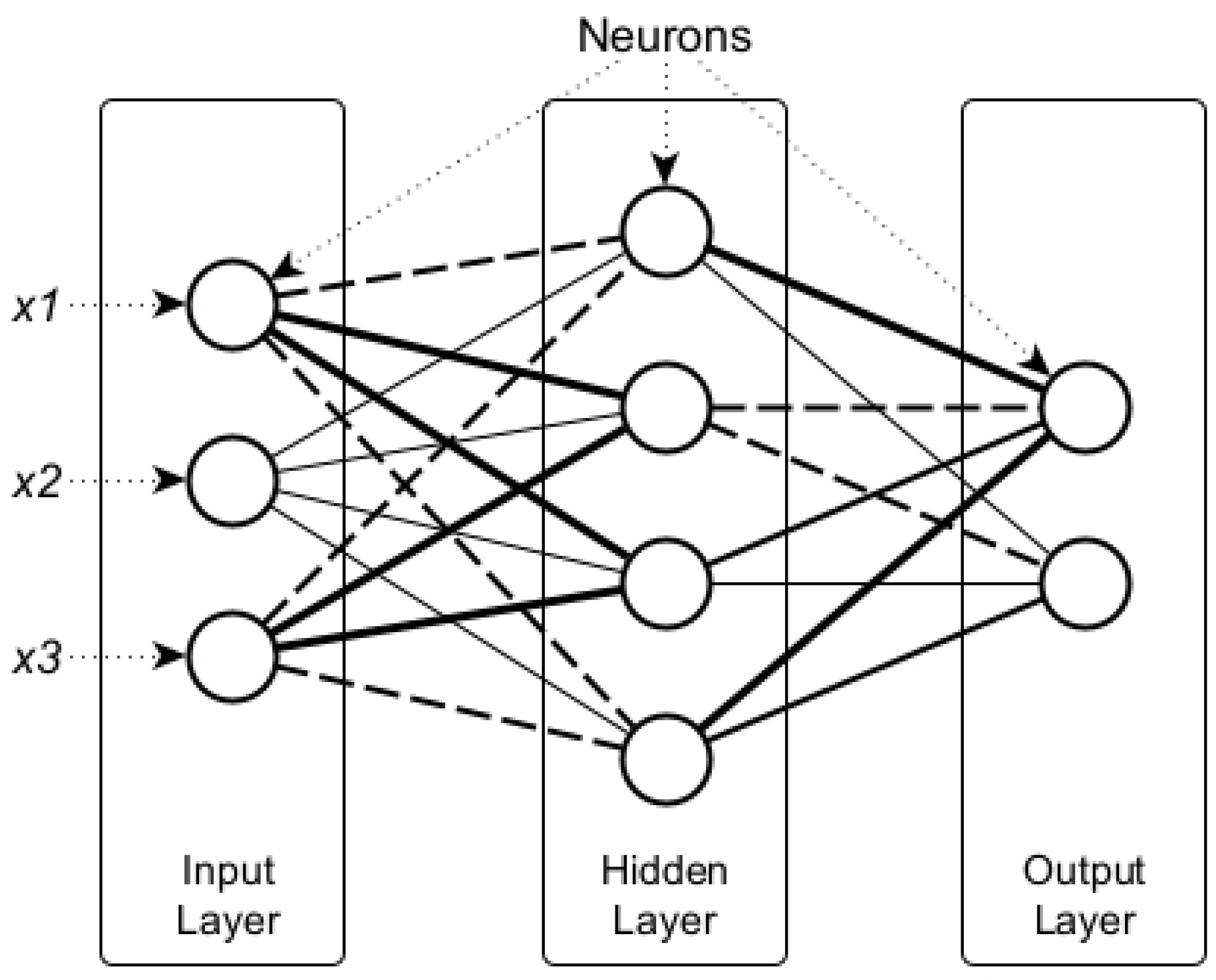
21]. Therefore, in the case of injection molding, the relationship of process parameters such as mold temperature, pressure, and cycle time with their corresponding output can be modeled and optimized by using ANN [22]. Nevertheless, modeling the nonlinearity within the data commonly leads to the complexity of the ANN itself. The increasing complexity of the ANN model is identified by the increasing number of hidden layers and neurons which represent more nonlinearity within the dataset. The complexity of the ANN model makes it well known as a “black box” model [23]. Despite the great success of ANN, the concern of a black box system has also received higher concern over time [24,25]. Black box interpretation prevents people from gaining understandable knowledge, which is essential for improving engineering design [26]. In terms of the injection molding process, having a better understanding of what factors have significant influence on the final results would give an advantage to the design of a better molding machine or technology.
Some studies have tried to infer significant process parameters of injection molding from the machine learning model. Zhou et al. [27] used an unsupervised approach named sparse autoencoder to cluster the learned parameter within the neural network training of various configuration injection molding experiments. Another study by Román et al. [28] used the Bayesian approach to optimize the parameter selection of deep neural network training for the defect prediction model of the injection molding surface. The developed model has successfully selected the parameter which yields the optimal model. A similar approach was proposed by Gim and Lee [29] by using interpretable machine-learning techniques to explain the significance of each injection molding parameter. A more innovative approach was deployed by using a transfer learning mechanism [30]. In that research, they deployed the deep neural network model which was successfully developed for another type of injection molding in their current experiment.
Regarding the efforts to develop better injection molding systems, there is much research that investigates the influential parameters of the molding process. Some researchers argued that cavity pressure has a significant parameter on the quality of injection molded products [31,32,33]. For instance, in an experiment conducted by Chen et al. [
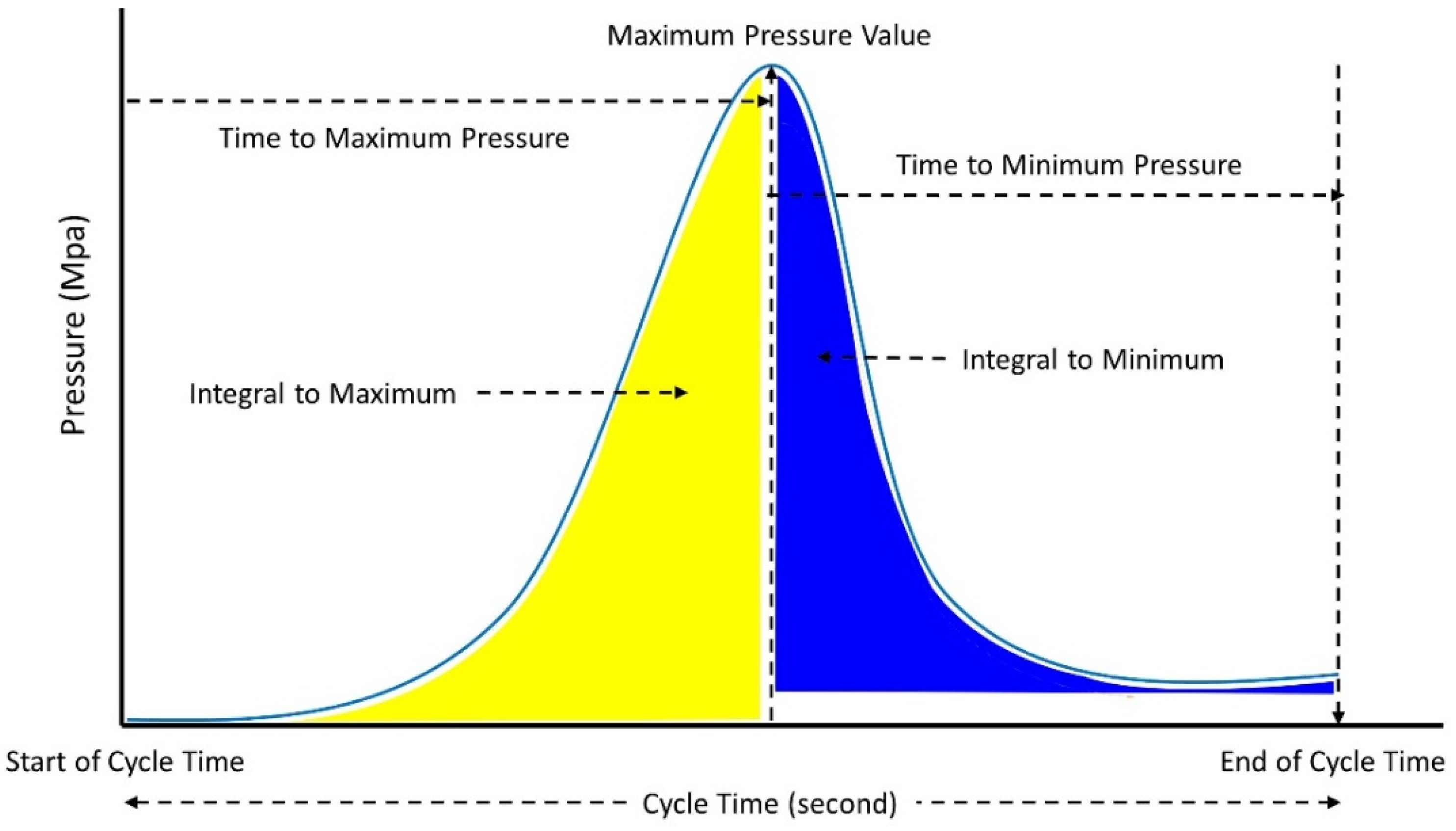
34], four cavity pressures, named peak pressure, gradient pressure, viscosity index, and energy index, were used to estimate the quality of injection molding output. In addition, Gim and Rhee [29] extracted five parameters from cavity pressure: initial pressure, maximum pressure, the integral value of pressure changes from the initial to the end of the process, final pressure at the filling stage, and final pressure from the cooling stage. Nevertheless, the determination of significant parameters is a difficult task which leads to the question of which parameters should be extracted from cavity pressure for accurate prediction [15].
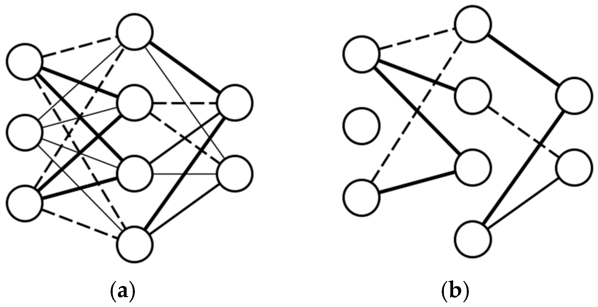
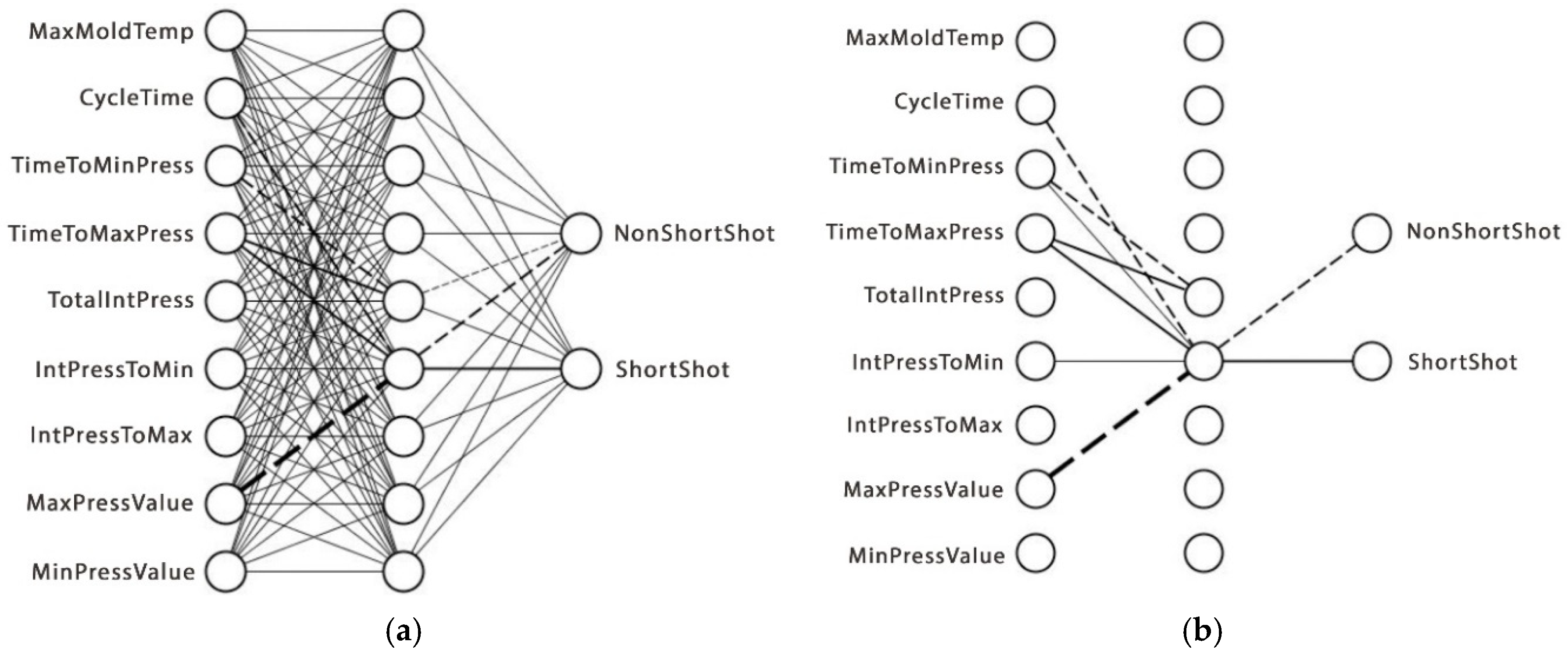
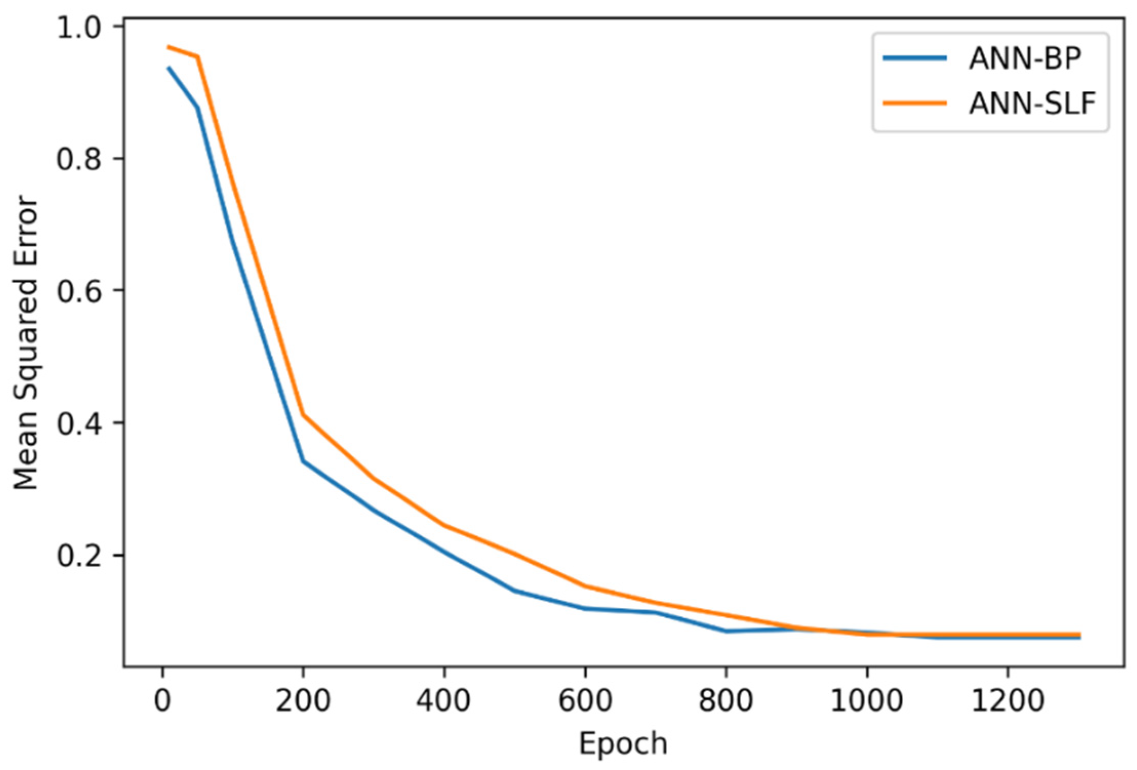
This experiment aims to provide an innovative approach to analyzing the significant attributes of the injection molding process by increasing the visibility of the ANN model. Since the ANN model has a good performance for injection molding quality prediction, reducing its model complexity without losing its performance hypothetically could reveal the injection molding variables as the input of the ANN model has the most significant influence on the prediction results. In this paper, an algorithm named structural learning with forgetting (SLF) was employed to train the ANN architecture. Different from the typical backpropagation algorithm commonly used in ANN training, SLF produced a simpler ANN model compared with the fully distributed model representation of the backpropagation training result. Hence, by using SLF for training the ANN model, significant parameters of injection molding which are represented as the input layer of ANN architecture can be further analyzed. The contributions of the present study can be summarized as follows:
(i).
We employed SLF to train the ANN model and generate a simpler model as well as to reveal the most significant attributes without any major degradation in prediction performance;
(ii).
We further analyzed the selected attributes to investigate the linear correlation among those attributes by constructing rules and evaluating the performance of the rules for quality prediction;
(iii).
We undertook in-depth experiments comparing the proposed model to other prediction models and findings from earlier research.
The remainder of this study is structured as follows. The dataset and detailed methods are presented in 
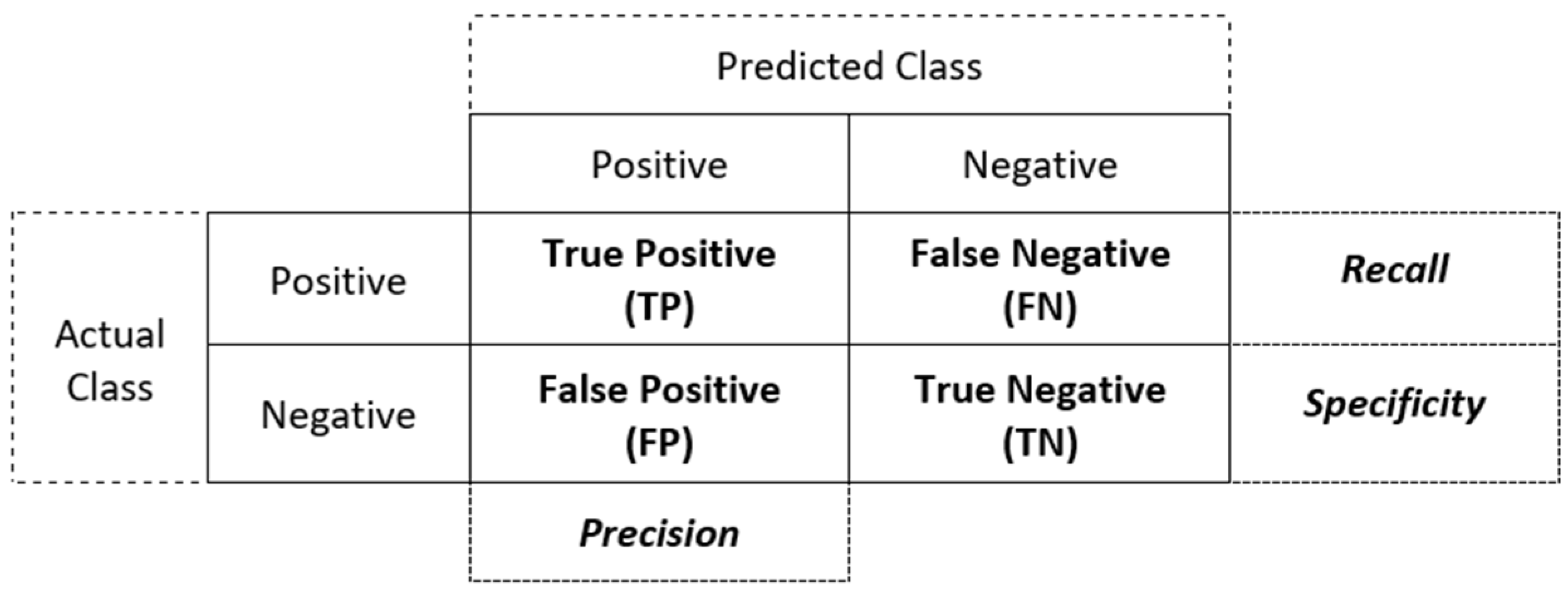
Section 2, including ANN, SLF, and the evaluation method. Section 3 provides comprehensive experimental results, parameter analysis with rule extraction, and comparison with earlier works. Section 4 presents the conclusion, including future research directions. Finally, the list of acronyms and abbreviations used in this paper are provided in the Abbreviations section.

2. Material and Methods

2.1. Dataset

The dataset used in this paper is gathered from the real injection molding process in our experiment. The data were collected using Argburg AllRounder 270 S hydraulic injection molding machine. This machine has a feature for online monitoring of process parameters through the graphical interface. With the machine interface, the cavity pressure and internal mold temperature can be investigated or even transmitted using a Kistler sensor. The experiment was conducted to produce a standard rectangular shape of product using LG Chemical’s ABS plastic material.
Table 1 outlines the attributes in our dataset which are derived from the injection molding process parameters followed by the illustration depicted in Figure 1 for better clarity of the phase of data collection for each attribute. In our dataset, there are 9 attributes and a class. The class attributes denote the results of the injection molding process. There are two class categories in our dataset, namely, defective (short-shot) and non-defective (non-short-shot). From the experiment data, the class label was determined by manually investigating the final plastic product of injection molding on each process instance. The non-defective class determines the ideal parameter value combination for generating good results in the injection molding process.
To infer the parameter values at various cavity pressures and mold temperature, the experiments were carried out with three different configurations for injection speed, switching the point of pressure holder and coolant temperature as shown in Table 2. Afterward, Table 3 explains the sequence of experiments based on the combination of the three different settings outlined in Table 2.
From the sequence of experiments shown in Table 3, each experiment was repeated 30 times, hence a total of 270 experiments were performed with different parameter configurations to produce a dataset that contains 270 instances. From the total number of data, 180 instances were used for training data (66.67%) and 90 instances were used for testing data (33.33%). To further investigate the values of each injection molding parameter, Table 4 provides descriptive statistics of the dataset used in this research.
From Table 4 we can see that the attributes on the dataset have different magnitudes. Some of the attributes have a large value and range, while others have relatively small values and range. Those kinds of differences will certainly lead to instability of the ANN training process. Hence, to standardize the value range of the attributes we need to normalize the attributes into the same value range. We then employ the Min-Max normalization approach to scale the dataset into the range of 0 to 1. The formulation of Min-Max normalization is depicted in the following Formula (1). In Formula (1), y defines the normalized data, while X = ( X 1 ,   ,   X 2 , , X n ) denotes the raw input of injection molding data on each attribute.
y i = X i min ( X ) max ( X ) min ( X )

2.2. Artificial Neural Network

An artificial neural network (ANN) is an approach to information processing by mimicking human nervous systems. ANN employs artificial neurons to transform a set of input values into a set of output values. An ANN is made up of a perceptron in the form of a node within a network to represent neurons of the human nervous system. Within ANN, a set of neurons are grouped into layers [24]. There are three kinds of a layer in ANN, namely, the input layer, hidden layer, and output layer. An ANN consist of at least one input layer to represent the input data and one output layer that represents the target output. A more complex ANN commonly has one or more hidden layers. Another part of ANN is connections between the nodes at different layers. Those connections or links have a weight value generated during the training process to determine the strength of the signal carried through the links [35]. The initial layer (or input layer) in this ANN is connected to the first hidden layer. Afterward, the output of the hidden layer feeds any more hidden layers that are directly transmitted to the output layer.
Multi-layered perceptron (MLP) is a type of ANN architecture that consists of fully connected neurons in feed-forward networks. Due to its robustness and performance, MLP is one of the most commonly used ANN architectures, either for research or practical purposes [36]. Figure 2 shows the example of ANN with MLP architecture with one input layer, one hidden layer, and one output layer. In the network, the diagram in Figure 2 depicts the lines representing the weight value. The thicker the line, the greater the weight value. The solid line depicts the positive weight value, while the dashed line depicts the negative value of the weight.
The values of the weights are determined by the operation within the neurons using an activation function. An activation function in a neural network describes how a node or nodes in a layer of the network translate the weighted sum of the input into an output. This function is a representation of the network’s method of information processing and transmission. Since there are different types of activation functions, different activation functions may be used in different regions of the model [37]. The choice of activation function has a significant impact on the neural network’s capacity and performance. Despite this, there is a need for a trial-and-error process to choose which activation to employ. The most commonly used activation functions, due to their derivative qualities which make training easier, are the linear, logistic/sigmoid, and hyperbolic tangent functions [38]. The formulation of these three activation functions is depicted in Equations (2)–(4), consecutively.
f ( x i ) = k x i
f ( x i ) = e x i 1 + e x i = 1 1 + e x i
f ( x i ) = 2 1 + e 2 x i 1 ,
During the ANN process, the weights on each neuron connection training are calculated iteratively. During the iteration process, the weight value will change according to the significance level of the connection to the accuracy of the prediction results [39]. The activation function is used to implement mathematical operators for weights. Furthermore, these values will be sent as a signal to the second hidden layer until it reaches the output layer. The value will be compared with the actual value in the data set after reaching the output count to calculate the prediction error. Finally, the learning process then iterates until the error is stable (the error value does not change).
There are various formulas for calculating the error of ANN prediction value during the training process. In this research, we use one of the most widely used error functions, namely, mean squared error (MSE). The calculation of MSE is done by using Equation (5). In Equation (5), N depicts the number of data on the dataset used for benchmarking the output prediction value, y ^ k represents the prediction value, and y k corresponds to the actual value on the training dataset.
M S E = 1 N   j = 1 N ( y k y ^ k ) 2

2.3. Structural Learning with Forgetting

The results of ANN prediction are well known for their accuracy. Nevertheless, since the prediction mechanism was hindered by its complex weight connection, it was uninterpretable by the user (black box process). Hence, inferring an interpretable rule from such network architecture required a complex process and plausibly led to a complex rule as the result. To overcome this drawback, an ANN training approach called structural learning with forgetting (SLF) was proposed by Ishikawa [40]. The SLF approach modifies the typical backpropagation learning algorithm by decaying the connection weight during the training process. Hence, the representation of the ANN model is much simpler. Structural learning methods are capable of generating skeletal structured networks with easy interpretation of hidden units instead of distributed representation which occurred during the backpropagation training.
The key idea of SLF is the forgetting of connection weights. During the learning with forgetting process, the connection weight which has no contribution to the learning process disappears leaving only the influential weight connection on the network architecture [41]. The remaining weight connections are a skeletal network that shows the regularity in training data. To implement the forgetting concept, the SLF-based neural network method defined a penalty term to the criterion function to favor the connection weights with small values. The criterion function in learning with forgetting is given by the following Equation (6) [42].
J f = J + ϵ   i , j | w i j | = i ( o i t i ) 2 + ϵ i , j | w i j |    
From the formulation of the above Equation (6), J f denotes total criterion. The penalty standard for J is then represented by the equation’s remaining parts. In this situation, J can be seen as being equal to the backpropagation method’s mean squared error. Afterward, ϵ represents the relative weight in the requirement for the forgetting criteria. The output of the i-th output unit is then represented by o i , the expected value is represented by t i , and the connection weight is represented by w , starting at a random value.
From the formulation depicted by Equation (6), the weight value of w is changed over time during the iteration of the training process. The change in the connection weight, w i j , is defined by Equation (7). In Equation (7), η is a learning rate, ϵ is the amount of forgetting at each iteration, and sgn(x) is the sign function (1 if x > 0 and −1 otherwise).
w i j = η   J f w i j = w ϵ   s g n ( w i j )
As learning progresses, the impact of initial connection weights also decreases. From Equation (7) it can be seen that for each connection it will lose weight each time the weight changes by the same amount of ϵ . Therefore, the word “forget” is used. Due to the forgetting process, the resulting network contains only the connections that significantly affect the final calculation of the output layer in the ANN architecture. Visually the difference between the regular network generated through backpropagation training and the trimmed network using the SLF technique are consecutively shown in Figure 3a,b below. From Figure 3b, we can roughly conclude that the ANN model produced by SLF training has a simpler representation.

2.4. Evaluation Method

The artificial neural network model has many parameters to be set within the training process, and one can use these parameters to perform specific tasks. To determine the best model, we used a set of evaluations to examine the prediction results during the learning process. The first evaluation is the confusion matrix. A confusion matrix is an exploratory evaluation approach that can be used to generally investigate how many true and false predictions are generated by any classification model [42]. There are four elements used in confusion metrics as explained in Table 5 which are also further used to calculate other evaluation metrics employed in this experiment.
From Table 5, in the case of injection molding quality prediction, the true positive results indicate that the model gave a correct prediction of the non-defective/short-shot results. The true negative occurred when the model correctly predicts the defective/non-short-shot results. Meanwhile, the false positive result indicates that the model predicts defective results while the actual value is non-defective. In the opposite direction, the false positive occurred when the model predicted non-defective results while the actual value was defective. From the elements explained in Table 5, we then constructed a confusion matrix. The format of the confusion matrix is illustrated in Figure 4.
The confusion matrix depicted in Figure 4 can be used to investigate the prediction quality of any classification task. The TP and TN boxes denote the correct prediction, whereas the FP and FN boxes indicate the wrong prediction. Therefore, the higher the values in TP and TN, the more accurate an ANN model results from the training process. We then used all of the elements (TP, FP, TN, and FN) on the confusion matrix to calculate a more meaningful evaluation of the ANN model. Four metrics can be derived from the confusion matrix, namely, precision, recall, specificity, accuracy, and F1-score [43].
The first metric derived from the confusion matrix is precision. Precision can be defined as the percentage of examples that are correctly identified as positive when a model predicts a positive class. The formulation of precision can be seen in Equation (8).
P r e c i s i o n = T P T P + F P  
The second evaluation metric is recall. Equation (9) formulates the calculation of recall. Recall defines the proportion of correct prediction of positive class to the total number of the positive class. The formulation of recall measures the sensitivity of the model since it compares the sum of correct predictions with the total number of incorrect predictions.
R e c a l l = T P T P + F N  
The third evaluation metric is specificity or the ratio of true negatives. In opposite to recall, specificity measures the percentage of correct prediction of negative class. The formulation specificity is defined by Equation (10).
S p e c i f i c i t y = T N T N + F P  
The next metric is the F-score which combines precision and recall to measure the overall performance of the model. In general cases, we need to make a trade-off between precision and recall. Hence, for a more general measurement, F-score takes a harmonic mean of precision and recall. Equation (11) shows the formulation of the F-Score.
F - s c o r e = 2 * P r e s i c i o n *   R e c a l l P r e c i s i o n + R e c a l l
The last metric is accuracy. The same as F-score, accuracy is used to measure the general performance of the model in a more straightforward way. The formulation of accuracy incorporates all of the confusion matrix elements as shown in Equation (12).
A c c u r a c y = T P + T N T P + F P + T N + F N   .

3. Results and Discussion

3.1. ANN Model of Injection Molding Quality Prediction

This section explains the results of the suggested SLF approach. In this study, the SLF technique and the typical backpropagation learning were run repeatedly to obtain the optimal parameter configuration. At first, to estimate the defects of plastic injection molding, a multi-layer perceptron neural network model was designed with an input layer, one hidden layer, and an output layer. A three-layer neural network is theoretically able to learn any non-linear relationship at the desired level of precision with a sufficient number of hidden neurons in the network. The model has nine input neurons, where the inputs can be the minimum pressure value (minPresVal), maximum pressure value (maxPresVal), integral pressure to maximum (intPresToMax), integral pressure to minimum (intPresToMax), total integral pressure (totIntPress), time to maximum pressure (timeToMaxPres), time to minimum pressure (timeToMinPres), cycle time (cycTime), and maximum mold temperature (maxMoldTemp). The output layer consists of two perceptrons, a value of 1 in the first perceptron and 0 in the second perceptron indicates defection (short-shot), whereas a value of 0 in the first perceptron and a value of 1 in the second perceptron indicates non-defect injection molding result (non-short-shot).
After several trial-and-error training runs to determine the optimal parameter, we have a parameter combination that reaches the minimum mean squared error (MSE) with a learning rate of n = 0.1, forgetting rate = 0.003, and the number of the hidden unit is 9. After the training process, we then compared the confusion matrix and the measurement metrics of the model obtained by backpropagation training and SLF training to show the efficacy of the suggested approach. Figure 5a shows the resulting structure of the neural network trained by using a typical backpropagation algorithm, and Figure 5b shows the resulting structure of the neural network trained using the SLF method. The solid lines represent the positive connection weight, while the dashed lines represent the negative connection weight. Then, the strength of the connections is represented by the line width.
The ANN model consists of a set of connections between neurons in their layer with their corresponding weights. Using backpropagation training, the connection weights of each connection remain at a certain value at the end of the training process. Whereas, by using SLF, the connection weights which have no significance to the final prediction fade away during the training process. Hence, when the connection weight is too small (e.g., under a certain threshold), the contribution to the output neurons was neglected. Furthermore, the remaining connection weights between the input and hidden layers show significant neurons in the input layer, namely, neurons in the input layer that still have connections with neurons in the hidden layer. Given that the neurons in the input layer represent the injection molding parameters, we can investigate which parameters of the injection molding process have a significant influence on the final quality prediction result.
Figure 6 illustrates the comparison of the MSE during the training process of the ANN model using backpropagation and SLF. The MSE of both algorithms have similar curves and start to converge to the minimum value of MSE on the 1000 epoch. The final value of MSE for backpropagation and SLF are around 0.075 and 0.079, respectively, which is a very small difference. Therefore, removing the weight connections of the insignificant attributes from the training process does not significantly decrease the model performance.
To assess the validity of the proposed approach, the performance evaluation of the two ANN models was furtherly compared. The evaluation criteria previously outlined in Section 2.4 were applied to both models. For evaluation purposes, the models were run to predict the test dataset which consists of 90 data. The first performance comparison is the confusion matrix as depicted in Figure 7. From Figure 7, we can see that there is no significant distinction between the confusion matrix of the ANN model trained with the backpropagation algorithm (see Figure 7a) and the ANN model trained with the SLF approach (see Figure 7b). The ANN model trained with the SLF algorithm made 6 errors (FP + FN) out of 90 predictions.
For further investigation, we then calculated the evaluation metrics based on TP/FP/TN/FN values on the confusion matrix on both models as presented in Table 6. To evaluate the models, the 10-fold validation mechanism was run and obtained the performance measures depicted in Table 6. From the evaluation comparison outlined in Table 6, even the backpropagation ANN model outperformed the SLF ANN model in all measurements, similar to the confusion matrix calculation, the value differences of each measurement of both models are not significant. Thus, by connection reduction in the ANN model, we have a simpler model with only significant attributes involved and good prediction performance.

3.2. Parameter Analysis with Rule Extraction

Investigation of the connection weights enables the extraction of significant attributes. Comparing the results from Figure 5a with Figure 5b indicates that when trained using the SLF method, five significant attributes were selected, in which one attribute has an extremely high influence on the final results. All other attributes vanished in the sense that all the incoming and outgoing connections from the corresponding hidden units faded away. The five significant attributes were maxPressValue, integralPressureToMin, timeToMaxPressure, timeToMinPressure, and cycleTime.
To validate the significance of extracted attributes, we then used those attributes to construct a rule for quality prediction. There are various methodologies for extracting rules over the resulting skeletal network by the SLF algorithm, ranging from the complex–systematic method to the simplest one, depending on the attributes involved and its values variation. For a complex problem (e.g., problems with a large number of attributes and each attribute having many possible categorical values) utilizing the Karnaugh map and representing every network’s units as a Boolean function is a suitable methodology for extracting the rules. Another rule, such as successive regularization, is suitable if we have only a few attributes but we must classify the problem into more than two classes. In this study, we used a rule extraction algorithm proposed by Setiono and Liu [44]. That rule extraction algorithm is operated over reduced/pruned ANN and designed for binary classification. Therefore, it is suitable for the ANN model built in this study using SLF for the training process.
At glance, the initial process of the rule extraction algorithm by Setiono and Liu [44] needs to consider the weighted path (the connection weight between the input neuron hidden neuron, and the connection weight between the hidden neuron and output neuron). If both connections are a positive connection or negative connection, then the multiplier on each attribute will be the positive value of its weight on the hidden layer ( + | w | ), otherwise, if the connection weight between the input to the hidden layer and between the hidden layer to the output layer is both different (one positive and one negative or vice versa) the multiplier will be the negative value of its absolute weight onto hidden layer ( | w | ). Then, we simply make a summation of each remaining attribute on each neuron with the following Equation (13).
i = 0 n ( w i *   x i ) > y
In the above formulation, w i is the connection weight from i-th input neuron to the corresponding hidden neuron, x i is the i-th-remaining attributes, and y is the summation result. For the two-class classification, we will get two y values from two classes. We pick one which has the best accuracy and then simply flip the inequality operator for classifying the other class. Then, as a result of the rule extraction algorithm over the resulting skeletal network trained with SLF, the conditional rules are obtained as outlined in Table 7.
We then evaluate the performance of the generated rules with an approach for measuring previous ANN models. The confusion matrix of the performance of the rules evaluation results is depicted in Figure 8 followed by the more detailed measurement results using the five evaluation metrics as outlined in Table 8.
The performance evaluation results of rule 1 and rule 2 in Table 8 shows that both rules remain with a fairly good score compared with the ANN models in Table 6. Figure 9 summarizes the performance comparison of the ANN models and the constructed rules. The graph depicted in Figure 9 shows that there are only small differences in the performance of the ANN models and the rules constructed from the selected injection molding parameters, which are considered highly influential.
To give additional insight, we provide the relative importance of each extracted parameter by SLF to the final prediction output in Figure 10. Figure 10 depicts how much the dismissal of each parameter from the initial ANN would decrease the model performance on each evaluation metric. For instance, the dismissal of the parameter “maxPressureValue” would decrease the model performance by around 0.22% or 22% from the “Recall” measurement.

3.3. Comparison with Earlier Work

We further investigated the performance of our models with earlier work that utilized the same injection molding dataset used in this study.
Syafrudin et al. [45] developed a big data framework and utilized the injection molding dataset to create the prediction models. They applied 10-fold cross-validation to the dataset and evaluated several machine learning models such as naive Bayesian (NB), multi-layer perceptron (MLP), logistic regression (LR), and random forest (RF). Their results showed that the highest accuracy score was achieved by RF (0.95), while the second, third, and fourth ranks belong to LR (0.92), MLP (0.89), and NB (0.67), respectively. In addition, they also revealed some significant features used in their study such as maxPressValue, integralPressureToMin, and TotalIntegral. Two-out-of-three features from their most important attributes are in line with our findings of significant features (i.e., maxPressValue, integralPressureToMin, timeToMaxPressure, timeToMinPressure, cycleTime) which also revealed that those attributes are most significant and contribute to the performance of the prediction models.
While Lee et al. [46] proposed an ontology-based quality prediction for injection molding, their study revealed that their proposed model can achieve an accuracy of up to 0.94. In the case of a feature, they also found that the maxPressValue attribute is also the most significant feature among others.
In general comparison, we discovered that our model achieved the highest accuracy of 0.97 for ANN-BPN (see Table 9). However, it is important to note that as the reported results were obtained using different methods, parameter settings, and validation techniques, comparing their direct performance does not provide accurate information. As a result, the results shown in Table 9 may not only be used to support the effectiveness of the categorization models but also to compare our study to earlier research in general.

4. Conclusions

In this study, an artificial neural network (ANN) model was trained using structural learning with forgetting (SLF). The SLF approach enabled us to reveal the most influential injection molding parameters by removing weak connections between the neurons during the training process. This mechanism leaves the strong connections and their corresponding input neurons within the ANN model at the end of the training process. Compared with the ANN model trained with a typical backpropagation training process, the ANN model trained using SLF has a simpler structure with less parameters as input with no major decline in terms of prediction performance. Thus, from the results, we can conclude the effectiveness of the proposed approach of using SLF to reveal the influential attributes.
Each of the input neurons represents a particular parameter of the injection molding process. Therefore, a process parameter represented by the remaining input neurons on the final ANN-SLF model is considered influential. There are five influential attributes extracted from this study, namely, Maximum Pressure Value, Integral Pressure to Minimum, Time to Maximum Pressure, Time to Minimum Pressure, and Cycle Time. Afterward, for further analysis, a set of rules for quality prediction was constructed to show the linear correlation between those process parameters. The evaluation method of those prediction rules shows that there are only small differences compared with the ANN models either trained using SLF or backpropagation. Hence, this experiment showed that by using SLF for training an ANN model and extracting rules over that model, the influential parameter of the injection molding process was successfully extracted without any major decline in terms of prediction performance. However, even though the distinction of the ANN-SLF model’s performance at all evaluation metrics is less than 7% comparing the best performer (ANN-BP and RF), this issue remained a drawback of our experiments and requires improvement in future works.
In the future, with the development of sensor technology, more parameters of the injection molding process can be monitored. Therefore, future work can involve more complex ANN architecture. Well-known deep ANN models such as convolutional neural networks, recurrent neural networks, etc., can be used for constructing prediction models using more process attributes and larger data. Hence, there is certainly a necessity to customize the training algorithm for model complexity reduction. Another effort for future work is to elaborate and explore the most significant attributes by using nature-inspired algorithms such as genetic algorithms and other parameter optimizations to gain the highest performance in predicting the quality of injection molding.

Author Contributions

Conceptualization, M.R.M. and Y.-S.K.; methodology, M.R.M. and R.F.L.; software, M.R.M. and R.F.L.; validation, M.R.M. and M.S.; investigation, R.F.L.; resources, M.R.M. and R.F.L.; data curation, M.R.M. and Y.-S.K.; writing—original draft preparation, M.R.M. and R.F.L.; writing—review and editing, M.S.; visualization, M.R.M. and M.S.; supervision, M.S. and Y.-S.K. All authors have read and agreed to the published version of the manuscript.

Funding

This research received no external funding.

Institutional Review Board Statement

Not applicable.

Informed Consent Statement

Not applicable.

Data Availability Statement

Not applicable.

Acknowledgments

Yong-Han Lee (Y.-H.L.) supervised the collection of the dataset that was used in this study. So, this article is a tribute to Y.-H.L., written out of the deepest respect for him, a genuinely good person and friend who served as our advisor and supervisor (1965–2017).

Conflicts of Interest

The authors declare no conflict of interest.

Abbreviations

List of abbreviations used in this study.
AbbreviationDefinition
CAEComputer aided engineering
ANNArtificial neural network
SLFStructural learning with forgetting
MSEMean squared error
TPTrue positive
FPFalse positive
TNTrue negative
FNFalse negative
LRLogistic regression
MLPMulti-layer perceptron
RFRandom forest
NBNaïve Bayes

References

  1. Kosior, E.; Mitchell, J. Chapter 6—Current Industry Position on Plastic Production and Recycling. In Plastic Waste and Recycling; Letcher, T.M., Ed.; Academic Press: Cambridge, MA, USA, 2020; pp. 133–162. ISBN 978-0-12-817880-5. [Google Scholar]
  2. Tosello, G.; Charalambis, A.; Kerbache, L.; Mischkot, M.; Pedersen, D.B.; Calaon, M.; Hansen, H.N. Value Chain and Production Cost Optimization by Integrating Additive Manufacturing in Injection Molding Process Chain. Int. J. Adv. Manuf. Technol. 2019, 100, 783–795. [Google Scholar] [CrossRef] [Green Version]
  3. Chen, Z.; Turng, L.-S. A Review of Current Developments in Process and Quality Control for Injection Molding. Adv. Polym. Technol. 2005, 24, 165–182. [Google Scholar] [CrossRef]
  4. Fernandes, C.; Pontes, A.J.; Viana, J.C.; Gaspar-Cunha, A. Modeling and Optimization of the Injection-Molding Process: A Review. Adv. Polym. Technol. 2018, 37, 429–449. [Google Scholar] [CrossRef]
  5. Moayyedian, M. Intelligent Optimization of Mold Design and Process Parameters in Injection Molding, 1st ed.; Springer Theses, Recognizing Outstanding Ph.D. Research; Springer International Publishing: Cham, Switzerland, 2019; ISBN 978-3-030-03356-9. [Google Scholar]
  6. Zhou, H. Computer Modeling for Injection Molding: Simulation, Optimization, and Control; Wiley: Hoboken, NJ, USA, 2013; ISBN 978-1-118-44488-7. [Google Scholar]
  7. Moayyedian, M.; Abhary, K.; Marian, R. The Analysis Of Defects Prediction In Injection Molding. Int. J. Mech. Mechatron. Eng. 2016, 10, 1883–1886. [Google Scholar] [CrossRef]
  8. Moayyedian, M.; Abhary, K.; Marian, R. The Analysis of Short Shot Possibility in Injection Molding Process. Int. J. Adv. Manuf. Technol. 2017, 91, 3977–3989. [Google Scholar] [CrossRef]
  9. Kurt, M.; Kaynak, Y.; Kamber, O.S.; Mutlu, B.; Bakir, B.; Koklu, U. Influence of Molding Conditions on the Shrinkage and Roundness of Injection Molded Parts. Int. J. Adv. Manuf. Technol. 2010, 46, 571–578. [Google Scholar] [CrossRef]
  10. Wibowo, E.A.; Syahriar, A.; Kaswadi, A. Analysis and Simulation of Short Shot Defects in Plastic Injection Molding at Multi Cavities. In Proceedings of the International Conference on Engineering and Information Technology for Sustainable Industry, Tangerang, Indonesia, 28–29 September 2020; Association for Computing Machinery: New York, NY, USA, 2020. [Google Scholar] [CrossRef]
  11. Li, D.; Zhou, H.; Zhao, P.; Li, Y. A Real-Time Process Optimization System for Injection Molding. Polym. Eng. Sci. 2009, 49, 2031–2040. [Google Scholar] [CrossRef]
  12. Hentati, F.; Hadriche, I.; Masmoudi, N.; Bradai, C. Optimization of the Injection Molding Process for the PC/ABS Parts by Integrating Taguchi Approach and CAE Simulation. Int. J. Adv. Manuf. Technol. 2019, 104, 4353–4363. [Google Scholar] [CrossRef]
  13. Primo Benitez-Rangel, J.; Domínguez-González, A.; Herrera-Ruiz, G.; Delgado-Rosas, M. Filling Process in Injection Mold: A Review. Null 2007, 46, 721–727. [Google Scholar] [CrossRef]
  14. Matin, I.; Hadzistevic, M.; Hodolic, J.; Vukelic, D.; Lukic, D. A CAD/CAE-Integrated Injection Mold Design System for Plastic Products. Int. J. Adv. Manuf. Technol. 2012, 63, 595–607. [Google Scholar] [CrossRef]
  15. Dang, X.-P. General Frameworks for Optimization of Plastic Injection Molding Process Parameters. Simul. Model. Pract. Theory 2014, 41, 15–27. [Google Scholar] [CrossRef]
  16. Michaeli, W.; Schreiber, A. Online Control of the Injection Molding Process Based on Process Variables. Adv. Polym. Technol. 2009, 28, 65–76. [Google Scholar] [CrossRef]
  17. Rousopoulou, V.; Nizamis, A.; Vafeiadis, T.; Ioannidis, D.; Tzovaras, D. Predictive Maintenance for Injection Molding Machines Enabled by Cognitive Analytics for Industry 4.0. Front. Artif. Intell. 2020, 3, 578152. [Google Scholar] [CrossRef]
  18. Bertolini, M.; Mezzogori, D.; Neroni, M.; Zammori, F. Machine Learning for Industrial Applications: A Comprehensive Literature Review. Expert Syst. Appl. 2021, 175, 114820. [Google Scholar] [CrossRef]
  19. Ageyeva, T.; Horváth, S.; Kovács, J.G. In-Mold Sensors for Injection Molding: On the Way to Industry 4.0. Sensors 2019, 19, 3551. [Google Scholar] [CrossRef] [Green Version]
  20. Zhang, Y.; Shan, S.; Frumosu, F.D.; Calaon, M.; Yang, W.; Liu, Y.; Hansen, H.N. Automated Vision-Based Inspection of Mould and Part Quality in Soft Tooling Injection Moulding Using Imaging and Deep Learning. CIRP Ann. 2022, 71, 429–432. [Google Scholar] [CrossRef]
  21. Ke, K.-C.; Huang, M.-S. Quality Prediction for Injection Molding by Using a Multilayer Perceptron Neural Network. Polymers 2020, 12, 1812. [Google Scholar] [CrossRef]
  22. Huang, Y. Advances in Artificial Neural Networks—Methodological Development and Application. Algorithms 2009, 2, 973. [Google Scholar] [CrossRef] [Green Version]
  23. Chen, J.C.; Guo, G.; Wang, W.-N. Artificial Neural Network-Based Online Defect Detection System with in-Mold Temperature and Pressure Sensors for High Precision Injection Molding. Int. J. Adv. Manuf. Technol. 2020, 110, 2023–2033. [Google Scholar] [CrossRef]
  24. Abiodun, O.I.; Jantan, A.; Omolara, A.E.; Dada, K.V.; Mohamed, N.A.; Arshad, H. State-of-the-Art in Artificial Neural Network Applications: A Survey. Heliyon 2018, 4, e00938. [Google Scholar] [CrossRef] [Green Version]
  25. Du, M.; Liu, N.; Hu, X. Techniques for Interpretable Machine Learning. Commun. ACM 2019, 63, 68–77. [Google Scholar] [CrossRef] [Green Version]
  26. Molnar, C.; Casalicchio, G.; Bischl, B. Interpretable Machine Learning—A Brief History, State-of-the-Art and Challenges. In Proceedings of the ECML PKDD 2020 Workshops, Ghent, Belgium, 14–18 September 2020; Koprinska, I., Kamp, M., Appice, A., Loglisci, C., Antonie, L., Zimmermann, A., Guidotti, R., Özgöbek, Ö., Ribeiro, R.P., Gavaldà, R., et al., Eds.; Springer International Publishing: Cham, Switzerland, 2020; pp. 417–431. [Google Scholar] [CrossRef]
  27. Zhou, X.; Zhang, Y.; Mao, T.; Ruan, Y.; Gao, H.; Zhou, H. Feature Extraction and Physical Interpretation of Melt Pressure during Injection Molding Process. J. Mater. Process. Technol. 2018, 261, 50–60. [Google Scholar] [CrossRef]
  28. Román, A.J.; Qin, S.; Zavala, V.M.; Osswald, T.A. Neural Network Feature and Architecture Optimization for Injection Molding Surface Defect Prediction of Model Polypropylene. Polym. Eng. Sci. 2021, 61, 2376–2387. [Google Scholar] [CrossRef]
  29. Gim, J.; Rhee, B. Novel Analysis Methodology of Cavity Pressure Profiles in Injection-Molding Processes Using Interpretation of Machine Learning Model. Polymers 2021, 13, 3297. [Google Scholar] [CrossRef] [PubMed]
  30. Lockner, Y.; Hopmann, C.; Zhao, W. Transfer Learning with Artificial Neural Networks between Injection Molding Processes and Different Polymer Materials. J. Manuf. Process. 2022, 73, 395–408. [Google Scholar] [CrossRef]
  31. Li, Y.; Yang, L.; Yang, B.; Wang, N.; Wu, T. Application of Interpretable Machine Learning Models for the Intelligent Decision. Neurocomputing 2019, 333, 273–283. [Google Scholar] [CrossRef]
  32. Rønsch, G.Ø.; Kulahci, M.; Dybdahl, M. An Investigation of the Utilisation of Different Data Sources in Manufacturing with Application in Injection Moulding. Int. J. Prod. Res. 2021, 59, 4851–4868. [Google Scholar] [CrossRef]
  33. Finkeldey, F.; Volke, J.; Zarges, J.-C.; Heim, H.-P.; Wiederkehr, P. Learning Quality Characteristics for Plastic Injection Molding Processes Using a Combination of Simulated and Measured Data. J. Manuf. Process. 2020, 60, 134–143. [Google Scholar] [CrossRef]
  34. Chen, J.-Y.; Yang, K.-J.; Huang, M.-S. Online Quality Monitoring of Molten Resin in Injection Molding. Int. J. Heat Mass Transf. 2018, 122, 681–693. [Google Scholar] [CrossRef]
  35. Baptista, D.; Morgado-Dias, F. A Survey of Artificial Neural Network Training Tools. Neural Comput. Appl. 2013, 23, 609–615. [Google Scholar] [CrossRef]
  36. Abiodun, O.I.; Jantan, A.; Omolara, A.E.; Dada, K.V.; Umar, A.M.; Linus, O.U.; Arshad, H.; Kazaure, A.A.; Gana, U.; Kiru, M.U. Comprehensive Review of Artificial Neural Network Applications to Pattern Recognition. IEEE Access 2019, 7, 158820–158846. [Google Scholar] [CrossRef]
  37. Samatin Njikam, A.N.; Zhao, H. A Novel Activation Function for Multilayer Feed-Forward Neural Networks. Appl. Intell. 2016, 45, 75–82. [Google Scholar] [CrossRef]
  38. Apicella, A.; Donnarumma, F.; Isgrò, F.; Prevete, R. A Survey on Modern Trainable Activation Functions. Neural Netw. 2021, 138, 14–32. [Google Scholar] [CrossRef] [PubMed]
  39. Zajmi, L.; Ahmed, F.Y.H.; Jaharadak, A.A. Concepts, Methods, and Performances of Particle Swarm Optimization, Backpropagation, and Neural Networks. Appl. Comput. Intell. Soft Comput. 2018, 2018, 9547212. [Google Scholar] [CrossRef]
  40. Ishikawa, M. Structural Learning with Forgetting. Neural Netw. 1996, 9, 509–521. [Google Scholar] [CrossRef]
  41. Pan, L.; Yang, S.X.; Tian, F.; Otten, L.; Hacker, R. Analysing Contributions of Components and Factors to Pork Odour Using Structural Learning with Forgetting Method. In Proceedings of the Advances in Neural Networks—ISNN 2004, Dalian, China, 19–21 August 2004; Yin, F.-L., Wang, J., Guo, C., Eds.; Springer Berlin Heidelberg: Berlin/Heidelberg, Germany, 2004; pp. 383–388. [Google Scholar] [CrossRef]
  42. Susmaga, R. Confusion Matrix Visualization. In Proceedings of the Intelligent Information Processing and Web Mining, Zakopane, Poland, 17–20 May 2004; Kłopotek, M.A., Wierzchoń, S.T., Trojanowski, K., Eds.; Springer Berlin Heidelberg: Berlin/Heidelberg, Germany, 2004; pp. 107–116. [Google Scholar] [CrossRef]
  43. Liu, Y.; Zhou, Y.; Wen, S.; Tang, C. A Strategy on Selecting Performance Metrics for Classifier Evaluation. Int. J. Mob. Comput. Multimed. Commun. (IJMCMC) 2014, 6, 20–35. [Google Scholar] [CrossRef]
  44. Setiono, R.; Liu, H. NeuroLinear: From Neural Networks to Oblique Decision Rules. Neurocomputing 1997, 17, 1–24. [Google Scholar] [CrossRef]
  45. Syafrudin, M.; Fitriyani, N.L.; Li, D.; Alfian, G.; Rhee, J.; Kang, Y.-S. An Open Source-Based Real-Time Data Processing Architecture Framework for Manufacturing Sustainability. Sustainability 2017, 9, 2139. [Google Scholar] [CrossRef] [Green Version]
  46. Lee, K.-H.; Kang, Y.-S.; Lee, Y.-H. Development of Manufacturing Ontology-Based Quality Prediction Framework and System: Injection Molding Process. IE Interfaces 2012, 25, 40–51. [Google Scholar] [CrossRef]
Figure 1. An illustration of data point collection of each attribute within a complete cycle of the injection molding process.
Information 13 00488 g001
Figure 2. Artificial neural network architecture with multi-layered perceptron.
Information 13 00488 g002
Figure 3. The difference between ANN architecture trained by using: (a) a backpropagation algorithm and (b) structural learning with a forgetting approach.
Information 13 00488 g003
Figure 4. Confusion matrix setup.
Information 13 00488 g004
Figure 5. The ANN model after being trained using: (a) a backpropagation algorithm and (b) structural learning with the forgetting approach.
Information 13 00488 g005
Figure 6. The mean squared error of ANN training using backpropagation and SLF.
Information 13 00488 g006
Figure 7. The confusion matrix evaluation of the ANN model is trained with (a) backpropagation and (b) structural learning with forgetting.
Information 13 00488 g007
Figure 8. The confusion matrix evaluation of (a) rule 1 and (b) rule 2.
Information 13 00488 g008
Figure 9. Performance comparison of ANN models and constructed rules.
Information 13 00488 g009
Figure 10. The comparison of extracted important parameters toward model performance.
Information 13 00488 g010
Table 1. The parameter of the injection molding process.
Parameter NameExplanationMeasurement Unit
Maximum Mold TemperatureMaximum temperature reach during the molding process on each cycle.Celsius
Cycle TimeThe time required for completing a single batch of the molding process from start to finish. A single batch of the molding process is recorded from the beginning of the molding process until the end of molded material ejection.Second
Maximum Pressure ValueMaximum cavity pressure value reached during the molding process on each cycle.Mpa
Minimum Pressure ValueThe minimum cavity pressure value was reached between the time when the maximum pressure value was obtained to the end of the injection molding process on each cycle.Mpa
Time to Maximum PressureTime required to reach the maximum pressure value from the start of the molding process on each cycle. Second
Time to Minimum PressureTime required to reach the minimum pressure value from the maximum pressure value of the molding process on each cycle. Second
Integral Pressure to MaximumThe integral value of the pressure change curve to reach maximum pressure from the start of the molding process on each cycle.-
Integral Pressure to MinimumThe integral value of the pressure change curve to reach minimum pressure from the start of the molding process on each cycle.-
Total Integral PressureThe integral value of the pressure change curve from the start to the end of the molding process on each cycle.-
OutputThis is the class label, 0 denotes short-shot, 1 denotes non-short-shot-
Table 2. The configuration factors for experiments.
Configuration FactorLevel 1Level 2Level 3
Injection speed (cm/second)345
Switching point of pressure holder (cm)1.522.5
Cooling water temperature (Celsius)103050
Table 3. The experimental settings.
Experiment NumberCooling Water TemperatureInjection SpeedSwitching Point of Pressure Holder
11031.5
21042
31052.5
43032
53042.5
63051.5
75032.5
85041.5
95052
Table 4. The parameter of the injection molding process.
Parameter NameMaxMinMeanStd. Dev.
Maximum Mold Temperature72.5823.4344.4618.57
Cycle Time22.4216.0219.131.52
Maximum Pressure Value290.3821.43134.4370.61
Minimum Pressure Value24.7903.334.71
Time to Maximum Pressure11.381.226.041.83
Time to Minimum Pressure16.5977.2613.081.59
Integral Pressure to Maximum946.3771.40364.8770.61
Integral Pressure to Minimum2764.4484.21717.89575.81
Total Integral Pressure3710.81288.121082.76663.55
Table 5. Element of ANN evaluation metrics.
AcronymElement NameExplanation
TPTrue PositiveThe ANN model correctly predicts the positive class.
FPFalse PositiveThe ANN model predicts the positive class as negative.
TNTrue NegativeThe ANN model correctly predicts the negative class.
FNFalse NegativeThe ANN model predicts the negative class as positive.
Table 6. Performance comparison of ANN model trained with backpropagation and SLF.
MetricsBackpropagationSLF
MeanStd. DeviationMeanStd. Deviation
Precision0.910.050.880.06
Recall10.040.940.04
F-Score0.950.050.910.05
Specificity0.950.060.930.07
Accuracy0.970.030.930.03
Table 7. Two rules were constructed from the selected injection molding parameters.
NoRule
1if (Maximum Pressure Value < 88.5) then: short-shot
otherwise: non-short-shot
2if (7.41 * Integral Pressure to Minimum) + (34.12 * Time to Maximum Pressure)
+ (28.14 * Time to Minimum Pressure) − (20.17 * Cycle Time)) > −2259) then: short-shot
otherwise: non-short-shot.
Notes: A multiplication is denoted by the sign (*).
Table 8. Performance evaluation of Rule 1 and Rule 2.
MetricsRule 1Rule 2
Precision0.820.88
Recall0.840.91
F-Score0.830.89
Specificity0.90.93
Accuracy0.880.92
Table 9. Comparison with earlier work that utilized the same injection molding dataset.
MetricsOur StudySyafrudin et al. [45]Lee et al. [46]
ANN-BPNANN-SLFRULE 1RULE 2NBLRMLPRFOntology-Based
Precision0.910.880.840.910.720.910.890.95-
Recall10.940.830.890.670.910.890.95-
F-Score0.950.910.90.930.650.910.890.95-
Accuracy0.970.930.880.920.670.910.890.950.94
Publisher’s Note: MDPI stays neutral with regard to jurisdictional claims in published maps and institutional affiliations.

