Article

Evaluation of Continuous Power-Down Schemes

Department of Computer Science, University of Nevada, Las Vegas, NV 89154, USA
*
Author to whom correspondence should be addressed.
Information 2022, 13(1), 37; https://doi.org/10.3390/info13010037
Submission received: 13 October 2021 / Revised: 14 December 2021 / Accepted: 10 January 2022 / Published: 13 January 2022
(This article belongs to the Special Issue Information Technology: New Generations (ITNG 2020 & 2021))

Abstract

:
We consider a power-down system with two states—“on” and “off”—and a continuous set of power states. The system has to respond to requests for service in the “on” state and, after service, the system can power off or switch to any of the intermediate power-saving states. The choice of states determines the cost to power on for subsequent requests. The protocol for requests is “online”, which means that the decision as to which intermediate state (or the off-state) the system will switch has to be made without knowledge of future requests. We model a linear and a non-linear system, and we consider different online strategies, namely piece-wise linear, logarithmic and exponential. We provide results under online competitive analysis, which have relevance for the integration of renewable energy sources into the smart grid. Our analysis shows that while piece-wise linear systems are not specific for any type of system, logarithmic strategies work well for slack systems, whereas exponential systems are better suited for busy systems.

1. Introduction

1.1. The Power-Down Problem and Online Competitive Analysis

The power-down problem is formally defined as follows: Consider here a system that has two states, called “ON” and “OFF”, and additionally a continuous or finite set of intermediate states. In the continuous case, the set of states is s [ 0 , 1 ] , where the value 0 is mapped to the ON-state; the value 1 is mapped to the OFF state; and the interval ( 0 , 1 ) is mapped to intermediate states. The running cost of the device in the ON state is proportional to the time of usage, while the device in the OFF state consumes zero amounts of energy; the intermediate states serve as sleep states, where the running cost is also proportional to time but has a smaller cost 0 < a ( s ) < 1 . There is no cost for switching from ON to OFF or any of the intermediate states, but a fixed cost 0 < d ( s ) < c occurs when switching from any of the intermediate states to ON, with c representing the cost of switching from OFF to ON. For systems with a finite number of states, instead of mapping from [ 0 , 1 ] , the states are { 0 , , k } , with 0 being the ON-state and k being the OFF-state.
At any time the device may be in any state but it must be swithced to the ON state when service is requested. Let t 1 s , , t n s and t 1 e , , t n e be non-negative real values that represent requests for service between the start of service times t i s and end of service times t i e , ( i = 1 , 2 , , n ) . Note that 0 t 1 s < t 1 e < t 2 s < t 2 e < < t n s < t n e holds. Thus, at time t i s , the state of a device must be in ON until time t i e . In between requests, the device can remain in the ON state, proceed to the OFF state or switch to any of the intermediate states.
We assume that as service requests are made our algorithm must determine how to switch the system without knowledge of future input. For the power-down problem, this means that an online algorithm will decide at each moment how to switch states without knowing what the next request will be. In contrast, an offline algorithm can make decisions based on the full knowledge of the entire input sequence. We say that algorithm A has competitive ratio C for a given request sequence σ , if the following is the case:
C o s t A ( σ ) c · C o s t opt ( σ ) ,
with C o s t A ( σ ) being the cost of A to serve σ and C o s t opt ( σ ) representing the cost of the optimal offline algorithm on σ . We say that algorithm A is has competitive ratio C if the inequality holds for all request sequences. Refer to Borodin and El-Yaniv [1] for a comprehensive treatise of online competitive algorithms.
Note that if t i e is very close to t i + 1 s , it may be inefficient for switching the device off. Instead, it would likely be advantageous to keep the machine switched on or perhaps to operate the device in any of the intermediate states. We also observe that during usage, the device must be ON—both offline and online—and worst case competitiveness is achieved for sequences where the length of the service t i e t i s is small and, in effect, infinitesimally short. The issue is whether the machine switches to a new state at time t i e . Under worst-case analysis, we will, thus, assume for our request sequences that the usage times of the device are infinitesimal: we redefine the input sequence as t i : = t i s = t i e , and we define a request sequence in terms of the arrival time of request i.
We summarize that for this problem the offline algorithm knows the duration of the idle time r i after request i until the next request and can, thus, pick the most cost effective state for this idle time. The online algorithm, however, has to decide on state transitions without knowledge of the length of r i .

1.2. Background and Related Work

Power-down mechanisms are common in electronic control from power optimization for hand-held devices to work stations to data centers. Power-saving states are routine for laptop computers and smart phones used in everyday life. See [2,3,4,5,6,7] for background of this research area.
However, the model is also useful for handling power-down phenomena in an emerging electrical grid, which predominantly relies on renewable energy; see our paper [8] for a survey on algorithmic approaches for a dependable smart grid. In that paper, we argue that game-theoretic approaches are essential for modeling the distributed smart grid, in the spirit of the approach taken almost four decades ago to model an emerging internet where requests are not driven by a well-defined distribution but are largely unpredictable.
The online competitive model has the advantage that statistical assumptions are not necessary. This is important for modeling a distributed smart grid, which incorporates renewables. In the traditional energy grid, when renewables produce a surplus of energy, such surplus generally does not affect the operation of traditional power plants. Instead, renewables are throttled down or the surplus is simply ignored. However, in the future, the majority of power is generated by renewables, and this is not tenable. Rather, traditional power plant output needs be throttled down or switched off in response to less predictable renewable supplies. Online competitive models have the advantage that little statistical insight is needed.
It be could argued that a game-theoretic approach that assumes an omniscient adversary may not be so realistic for modeling the grid; however, this kind of modeling provides performance guarantees in the absence of reliable forecasting. For example, climate scientists have noted unusual weather patterns related to a change in Arctic Oscillation (OA) and North Atlantic Oscillation (NAO) [9]. Recently, unprecedented winter storms across Texas in February 2021 caused wide-spread power outages [10]. See also Maimó-Far et al. [11] for unpredictability issues around renewables. In order to guarantee a resilient grid, worst case assumptions must be taken into account.
In [12], we have extensively studied the power-down problem when there is a finite number of intermediate power states. For that discrete version of the power-down problem, we have also developed adaptive algorithms (see [13]). In our recent journal paper [14], we have developed a decrease and reset technique that responds to the frequency of requests by increasing idle times as requests become sparse.
In a majority-renewables grid, power gaps may be filled by a limited number of fossil fuel generation plants, such as gas turbines [8]. Guelen [15] points out that “the most efficient, clean, and fast-responding power-plants are natural gas-fired turbine power plants”. There is now extensive interest in gas turbines (see the recent handbook by Winterbone and Turan [16]). Such turbines come in many guises but a commonality is that throttling is continuous rather than finite.
Our paper expands our work on finite state systems given in [12] to continuous scenarios. The paper provides a unified framework based on earlier studies presented at previous ITNG meetings [13,17,18], but simulations in this paper are geared towards modeling throttling traditional power plants in a majority-renewables smart grid. We consider an abstracted set of functions that scale to a wide range of systems and compare three different strategies, namely “exponential”, “logarithmic” and “piecewise linear” under competitive analysis. From our analysis, we derive policies that are suited best for different scenarios, such as a highly fickle system or a system with a high degree of slack.

1.3. Organization of Paper

Our paper is organized as follows: In Section 2, we provide the continuous state model and define corresponding idle and power-up costs. The functions are motivated by the control of gas turbines in a majority-renewables grid. Section 3 solves the power-down problem for the model when all requests are known in advance. In Section 4, we provide general results for online strategies and analyze in the next two sections (Section 5 and Section 6) two specific parameterized strategies—namely logarithmic and exponential—that are both useful in practice. We provide further simulation results regarding logarithmic and exponential strategies in the Appendix A. Section 7 discusses the piece-wise linear strategy, which is useful but simpler. In both sections, we provide a comprehensive analysis of competitive ratios. Section 8 provides quantitive analysis of the strategies. Section 9 places our results into further perspectives.

2. The Power Model

We study a continuous power model with a set of states { s R | 0 s 1 } ; each state has an associated idle cost a ( s ) and power up cost d ( s ) —the switching cost to the “ON” state that is indexed by 0. As mentioned before, the model considered here is motivated by the cycling of gas turbines. Gas turbines can be throttled to different levels of power generations. Today, they are often still used in combination with steam turbines to make a combined cycle gas turbine power plant. The temperature range of the combined cycle is greater than the range of either of the individual components, and load control can be achieved by changing the number of gas turbines coupled to the steam turbine [16]. Thus, the idle cost and power up cost may be quite different across different types of turbines. We will consider here a generic system, with idle cost function a ( s ) and power up cost function d ( s ) as follows.
a ( s ) = 1 s a
d ( s ) = c s d
The system models various real-world situations, such as the powering up of a power plant, where the power cost decreases at a polynomial rate as the system throttles to a lower state, and the power up cost increases at a polynomial rate as the system throttles down. Such a system can be used to model a wide variety of situations. We mention that state 0 is the highest power “ON” state, state 1 is the “OFF” state and all real numbers between 0 and 1 are intermediate states (c.f. Figure 1a). For modeling, we choose somewhat arbitrarily values including a = 5 , c = 1 and d = 5 . We will describe below that with this choice of parameters we can describe important qualitative differences of various online strategies, and we demonstrate in the the Appendix A that these characteristics remain valid for a variety of other parameter choices.
We will also discuss the special case of a linear system provided by the following:
a ( s ) = 1 s
d ( s ) = c s ,
where, as before, we chose somewhat arbitrarily c = 1 (c.f. Figure 1b). We will refer to the system of Figure 1b as the “Linear System” and the system of Figure 1a as the “General System”.

3. Offline Strategy

The optimal offline algorithm chooses a state that minimizes cost r · a ( s ) + d ( s ) . We can minimize this cost by using r · a ( s ) + d ( s ) d y d s = 0 , we then solve for s, which we rename Strategy OFF , which is a function of r as follows:
Strategy OFF ( r ) = a · r d · c 1 d a
where r is the idle duration. We choose a state when the machine would proceeds to be idle and remains in this state for r units before power up to the “ON” state. The cost of the offline algorithm can be shown by the following.
Cos t OFF ( r ) = r · a ( Strategy OFF ( r ) ) + d ( Strategy OFF ( r ) )
We use Equation (6) to determine the point in time when the offline algorithm would utilize the “OFF” state throughout its idle duration by setting the equation to 1, i.e., the “OFF” state. We denote this “threshold” time as τ .
a · τ d · c 1 d a = 1
τ = c · d a
Thus, if r τ , the offline strategy would remain “OFF” throughout the idle duration in order to be optimal. We note that, for the linear system, offline strategy utilizes the “ON” state throughout idle time until time τ .

4. Online Strategies

We analyze a set of possible online strategies for the power model introduced in Section 2. As noted before, an online algorithm cannot make assumptions about future events; thus, the time spent idle is unknown. An online algorithm starts at the highest power state (“ON” or 0) the moment the machine becomes idle and begins powering down to lower power states until the request arrives. The power up cost from the state that the online algorithm is using is then incurred to the power cost of being idle. If we have some online strategy Strategy ON , then its cost is as follows.
Cos t ON ( r ) = 0 r a ( Strategy ON ( u ) ) d u + d ( Strategy ON ( r ) )
Using Equations (7) and (10), we can compute the competitive ratio.
Competitive Ratio = max 0 r τ Cos t ON ( r ) Cos t OFF ( r )
Equation (11) provides us with the competitive ratio for each request with wait time r.
Theorem 1.
For any continuous online strategy, once the wait time reaches τ, online strategy powers down in order to minimize its competitive ratio.
Proof. 
We set up the proof by contradiction that, when the idle time is τ , the online strategy does not power down. This strategy is optimal. Thus, the machine switches to the “OFF” state either before or after τ . The trivial case is when the machine powers down after τ or r > τ . Then, from Equation (10), we have the following competitive ratio:
0 τ + δ a ( Strategy ON ( u ) ) d u + d ( Strategy ON ( τ + δ ) ) 1 .
where δ > 0 , the offline algorithm choses the “OFF” state throughout the idle duration and δ increases the online cost, consequentially increasing the competitive ratio. The other case where online strategy powers down before the τ would yield the following competitive ratio using Equations (7) and (10).
0 τ δ a ( Strategy ON ( u ) ) d u + 1 r · a ( Strategy OFF ( τ δ ) ) + d ( Strategy OFF ( τ δ ) ) .
We substitute 1 for d ( Strategy ON ( τ δ ) ) for the power up cost since the online strategy powers down at some time τ δ , where δ > 0 . For any δ value , d ( Strategy ON ( τ δ ) ) < 1 —thus, the online cost will incur an extra cost of 1 d ( Strategy ON ( τ δ ) ) when powered down before τ . Consequently, online cost becomes larger so the competitive ratio is not minimal. Thus, the competitive ratio can only be minimal if online strategy powers down at when the idle duration is τ . □
In the next sections, we analyze various online strategies.

5. Logarithmic Strategies

We use the following function as a template for a set of logarithmic strategies:
Strategy ln ( r ) = ln Λ r ln Λ τ
where r is the idle time, τ is the threshold time where the machine would power down to the “OFF” state and Λ is a control parameter that controls the transition rate. Each online strategy has a different Λ value.
Figure 2a and Figure 3b are the same set of online strategies applied on the general system and linear system, the competitive ratios can be seen in Figure 2b and Figure 3b, respectively. The logarithmic strategy switches to lower power states rapidly at the beginning of the idle period and then slowly as the duration reaches τ . We observe that competitive ratios are maximal at the beginning of the idle durations and then decreases to its minimal competitive ratio when the idle duration reaches the value of τ . We see this pattern when logarithmic strategy is applied on both the general and linear system; however, the results are more extreme in the linear power system.

6. Exponential Strategies

For exponential strategies, we use the following function template the following:
Strategy exp ( r ) = e Λ r 1 e Λ τ 1
where r is the idle time, τ is the threshold value and Λ is the control parameter that determines the transition rate. Using a set of Λ values, we can construct different online strategies, where each strategy transitions to lower power states at an exponential rate.
Figure 4a and Figure 5b show exponential strategies used in the experimentation. For exponential strategies, we see transition rate changes gradually, then towards the end of the idle period, the transition increases rapidly. The competitive ratios for these strategies on a general and linear system are shown in Figure 4b and Figure 5b, respectively. In both power systems, we can notice similar patterns, where the competitive ratio is minimal at the beginning of the idle period. Then, it increases throughout the idle duration and is maximized when the duration is τ , with the exception of one of the strategies when Λ is large when experimenting in the linear system.
When compared to the logarithmic strategy, we see that the two systems are rather opposites of each other. Logarithmic strategies are at their maximum at the beginning of the idle period and then become minimal towards the end, and the exponential strategies are minimal at the beginning and reach its maximum towards the end. The experiments suggests that exponential strategies are more favorable overall, since the maximal competitive ratio is achieved towards the end and only for a short duration, and for the majority of the time spent idle it has a favorable competitive ratio. However, even though the logarithmic strategies are larger than the exponential strategies for the most part, the competitive ratios of logarithmic strategies are favorable at time τ . Thus, idle durations are consistently large, then the logarithmic strategy is favorable; however, in most of the cases, the exponential strategies are favorable.

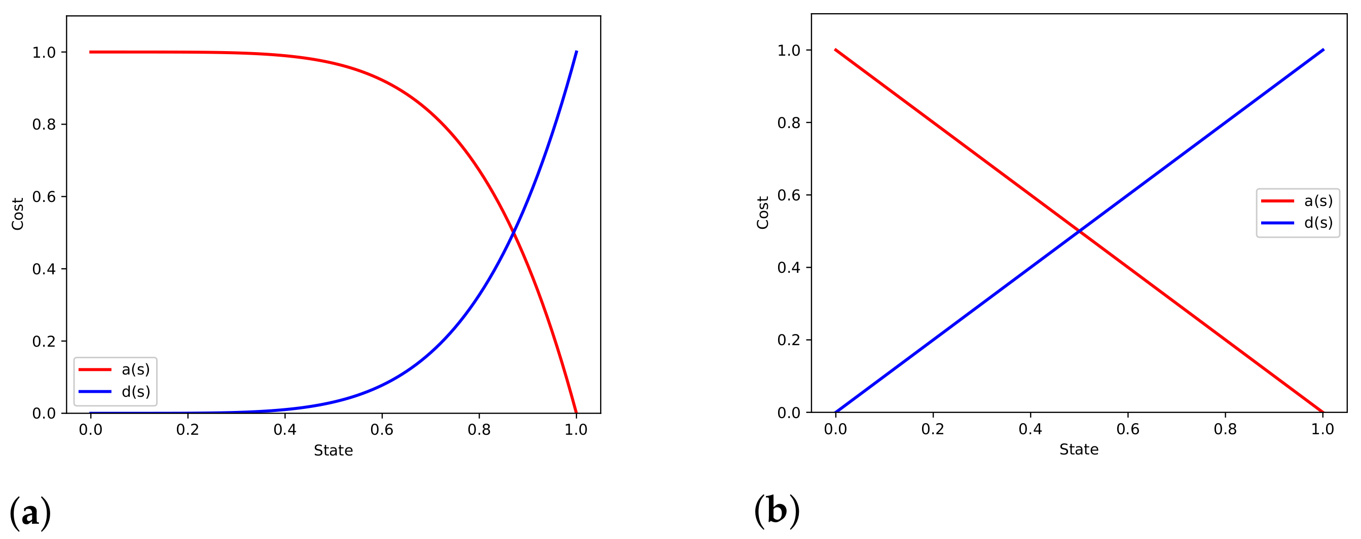
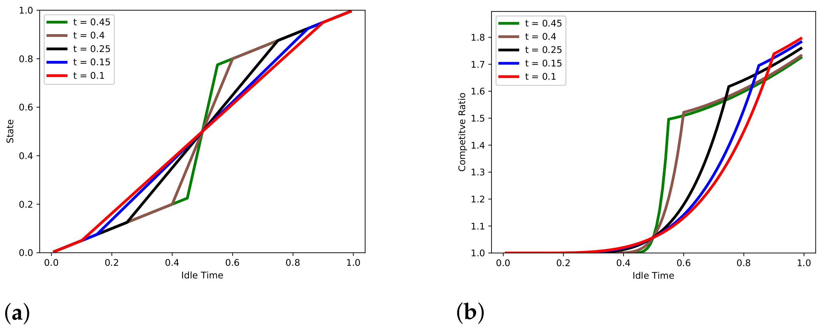
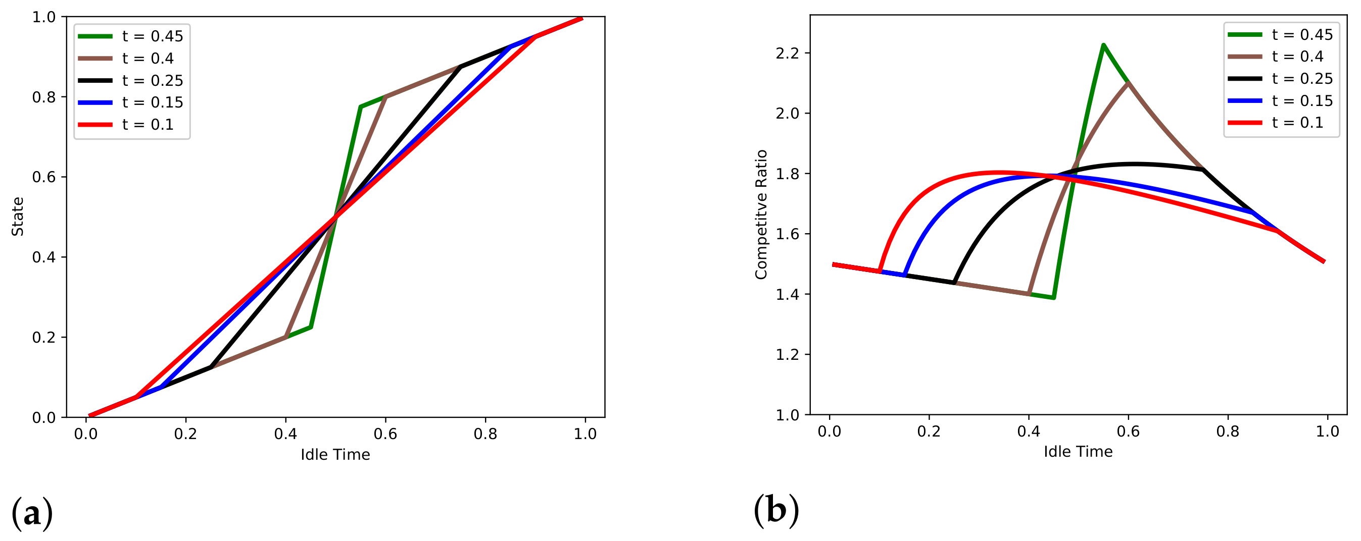
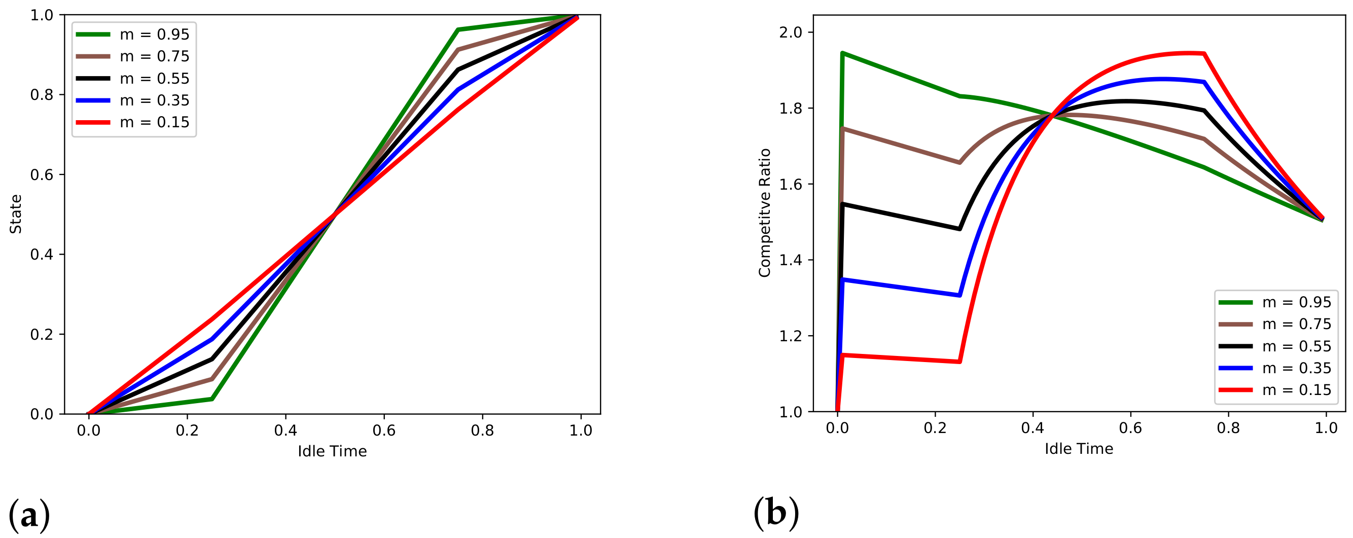
7. Piece-Wise Linear Strategies

The previous strategies—exponential and logarithmic—had the pattern of either transitioning at a slower rate earlier in the idle period and then transitioned at a faster rate towards the end of the idle period and vice versa. This online strategy uses two control parameters: a given slope m and the given amount of time t spent at the beginning and end using transition rate m. Using the given transition rate m, the strategy would transition to lower power states during the duration [0, t], which can also be denoted by [0, x 1 ]; then, a new transition rate m is computed, and the online strategy transitions at rate m in durations (t, τ 2 t ], which we can denote this duration ( x 1 , x 2 ], and then strategy transitions at rate m once again for t units in the duration ( τ 2 t , τ ], which we denote ( x 2 , τ ] . We use the three linear functions to model this strategy:
f 1 ( r ) = m r
f 2 ( r ) = m r + b
f 3 ( r ) = m r + τ m
where m = 2 m ( 1 t ) + 1 1 2 t and b = t ( m m ) . We then can construct the following piece-wise linear function below.
Strategy ON = f 1 ( r ) if r x 1 f 2 ( r ) if x 1 < r x 2 f 3 ( r ) if x 2 < r < τ 1 if r τ
Since we have two given control values m and t for the piece-wise linear strategies, we conduct experiments where, in our first experiment, we choose a transition rate m and cycle through a set of t values, and then, for the other experiment, we choose the duration t and cycle through a set of transition rates.
Figure 6a and Figure 7a show the strategies used for experimentation. For all strategies, we chose m = 0.50 and cycled through a set of t values, the competitive ratios when we run these strategies on a general and linear power system can be observed in Figure 6b and Figure 7b, respectively. For the general power system, we observe a similar behavior as with the exponential strategy where the competitve ratio is minimal at the beginning of the idle duration and rapidly increases from x 1 to x 2 and then gradually increases from x 2 to τ .
For the linear system, the competitive ratio surges at the beginning but decreases gradually from 0 to x 1 ; then, the competitive ratio increases in duration x 1 to x 2 for some of the strategies where x 1 to x 2 is a larger duration and, thus, has a smaller m transition rate. The competitive ratio decreases as the duration is approaching x 2 , and then from x 2 to τ , the competitive ratios decrease. For general and linear power systems, the pattern that we can observe is that the competitive ratio values are similar at the beginning and converge to similar results at the end, but the strategy with the larger t, which results in a smaller duration from x 1 to x 2 , causes a larger m transition rate that has a larger competitive ratio during that x 1 to x 2 duration. Thus, the conclusion is that the strategy that uses a larger t value results in the largest competitive ratio and, thus, the least favorable strategy.
Figure 8a and Figure 9b are online strategies applied on a general and linear system. In these strategies, we chose a fixed t duration for all strategies, and we cycle through a set of transition rates m during the beginning and ending intervals. The competitive ratio shown in Figure 8b shows the minimal competitive ratios at the beginning and then increases towards the end, similar to the exponential strategy shown earlier. However, we observe that the strategy with the larger m and larger m value is minimal throughout the idle duration except at time τ , and the strategy with the smallest m and m has the largest competitive ratio except at time τ . Overall, the strategy with the largest m value has the favorable competitive ratio for the majority of the idle time.
When the same set of online strategies are simulated on a linear power system shown in Figure 9b, they all have a surge in competitive ratio at the very beginning, then most of the strategies decrease after the surge, and then they increase after x 1 , then the competitive ratios decrease as the idle time approaches x 2 , and then the strategies all decrease their competitive ratios from x 2 to τ , with the only exception to the strategy being the largest m value. The strategy with the better competitive ratio at the beginning is the strategy with the smallest m value, then the second half of the idle period the strategy with the larger m value has a better competitive ratio.

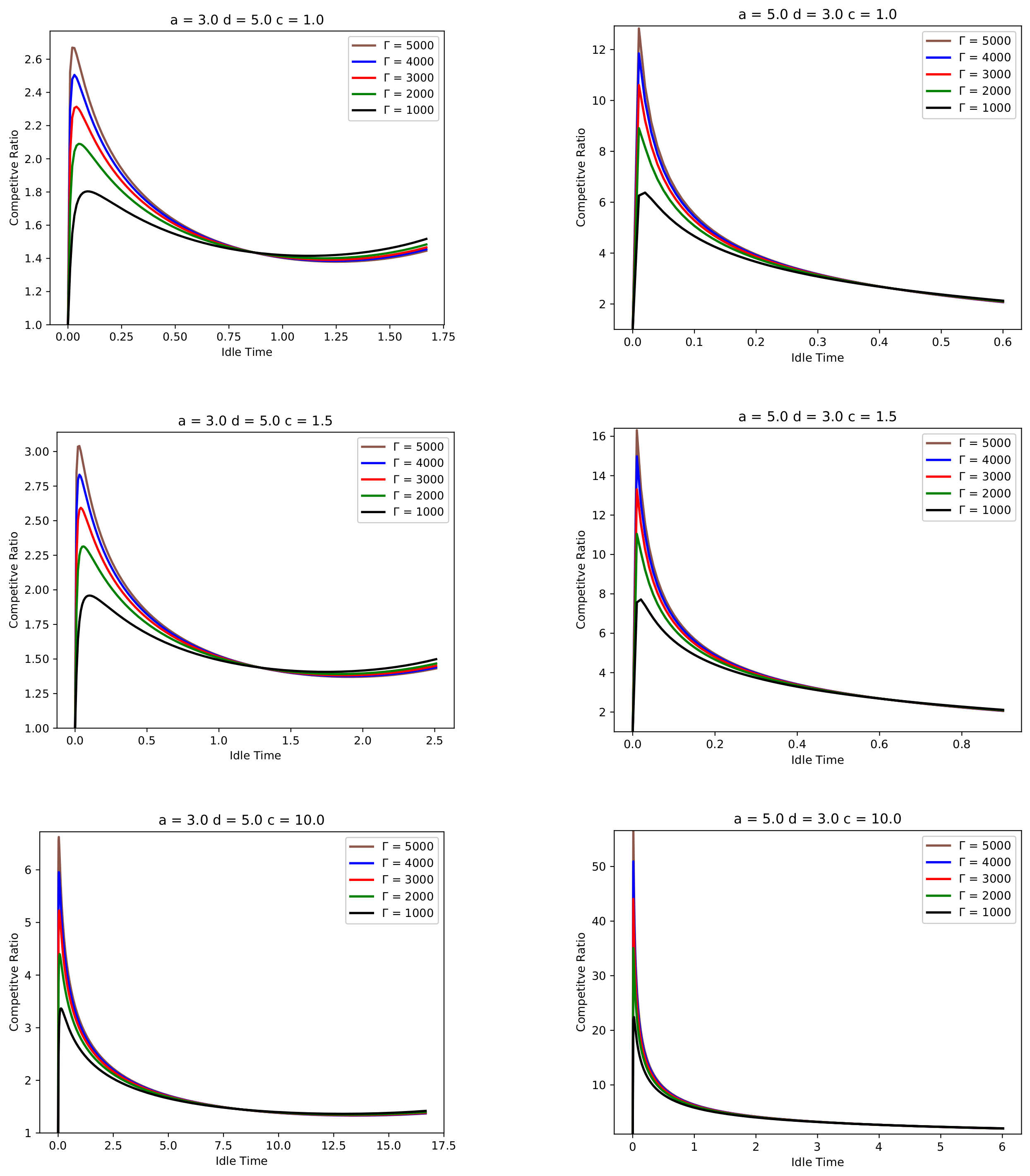
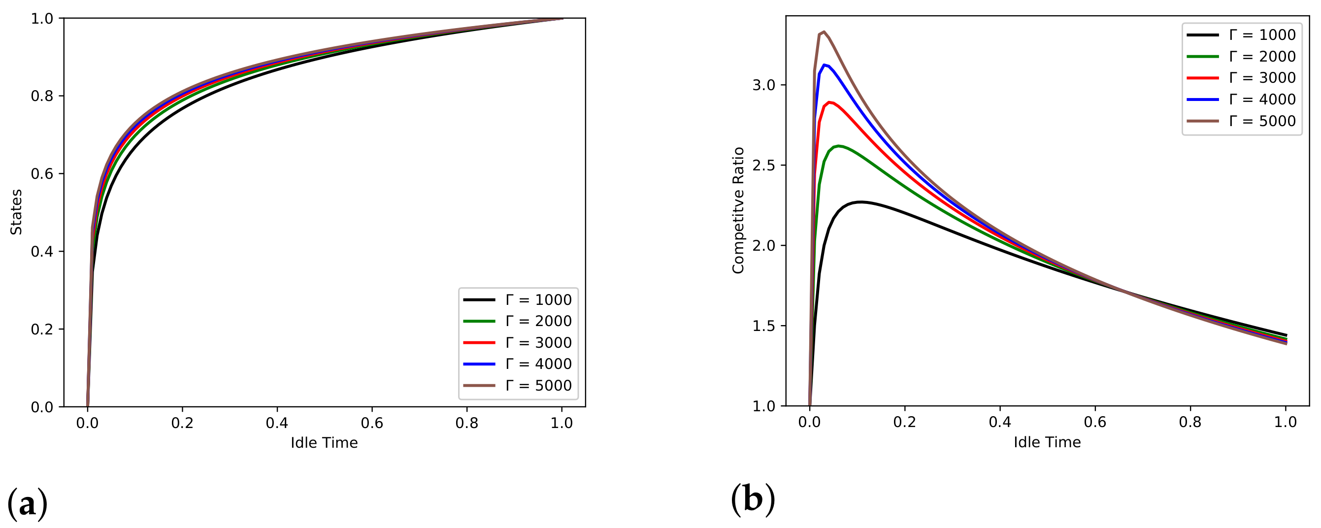
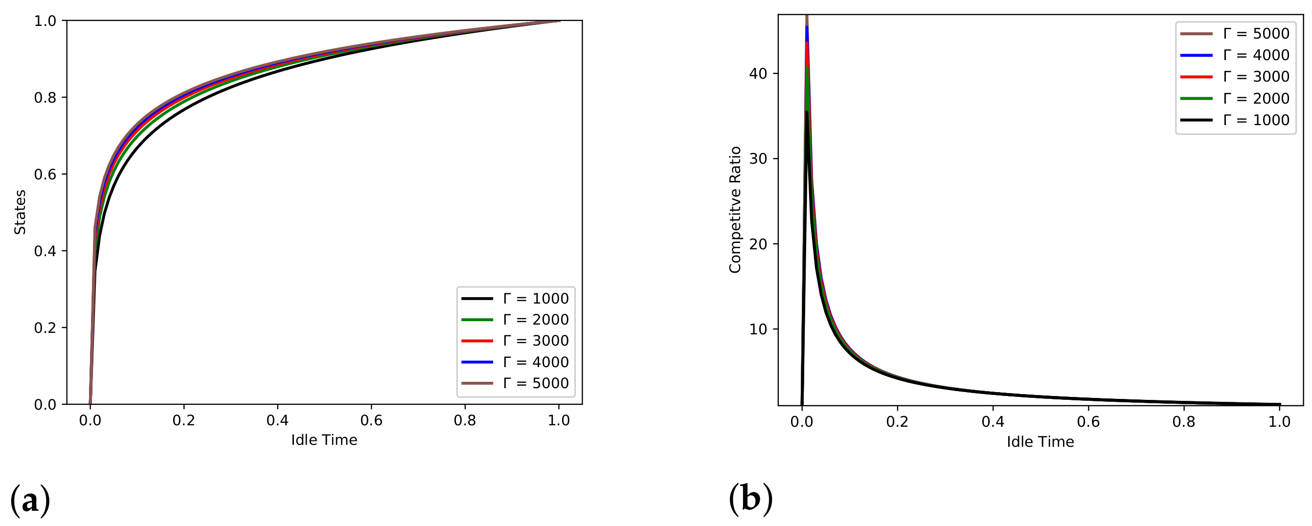
8. Comparative Analysis

In [14], we have defined the notion of a slackness degree. Roughly speaking, a system is slack, if requests seldom arrive, and a system is busy if requests arrive in quick succession. We argued that it important to analyze systems for the worst case; in that sense, one would not classify competitive results in terms of being slack or busy. However, in practice, a worst-case analysis that takes into account this single property is very useful.
Looking at the general system, Figure 3 shows that the competitive ratio is favorable when the idle time is larger than 0.5 . On the other hand, exponential strategies (see Figure 5) exhibit the opposite characteristic: the competitive ratio is favorable when idle times are less than 0.5 . Figure A1 and Figure A2 in the Appendix A show this to be present for various systems with different parameter values.
For piecewise-linear strategies, observations are not as easily classified, but generally those strategies are more akin to exponential strategies. However, by setting up the slope carefully, the behavior can be finetuned to more specific characteristics.

9. Conclusions

A choice of logarithmic, exponential and piece-wise linear strategies was modeled on a linear as well as a more general power system. From our work, we observe that there is no one best strategy. Every strategy on each power system had periods where it had favorable competitive ratios and instances where the competitive ratios would be large. The highest competitive ratio for that strategy on a power system is considered the competitive ratio for the strategy. However, the worst-case may not be the most important consideration for real-world applications. Thus, our results can guide strategy choices depending on the application.
Our work is important for the integration of fossil fuel power plants into a majority-renewables electrical grid. The fickle nature of solar and wind power is often cited as a major impediment for the speedier adoption of renewables. Online competitive models play an important role in creating a resilient renewable grid.

Author Contributions

The two authors contributed equally to this paper. All authors have read and agreed to the published version of the manuscript.

Funding

The work of author Wolfgang Bein was supported by the National Science Foundation, Grant IIA 1427584. This author also acknowledges a sabbatical granted by the University of Nevada, Las Vegas, for the 2021/22 academic year, which benefited this project.

Institutional Review Board Statement

Not applicable.

Informed Consent Statement

Not applicable.

Data Availability Statement

The data that support the findings of this study are available from the corresponding author upon reasonable request.

Conflicts of Interest

The authors declare no conflict of interest.

Appendix A

1. Simulations Parameter Values and Logarithmic Strategy
Figure A1. Simulations logarithmic strategies for various parameter values.
Information 13 00037 g0a1
2. Simulations Parameter Values and Exponential Strategy
Figure A2. Simulations exponential strategies for various parameter values.
Information 13 00037 g0a2

References

  1. Borodin, A.; El-Yaniv, R. Online Computation and Competitive Analysis; Cambridge University Press: Cambridge, UK, 1998. [Google Scholar]
  2. Agarwal, Y.; Hodges, S.; Chandra, R.; Scott, J.; Bahl, P.; Gupta, R. Somniloquy: Augmenting Network Interfaces to Reduce PC Energy Usage. In Proceedings of the USENIX Symposium on Networked Systems Design and Implementation (NSDI ’09), Boston, MA, USA, 22–24 April 2009; pp. 365–380. [Google Scholar]
  3. Agarwal, Y.; Savage, S.; Gupta, R. Sleepserver: A software-only approach for reducing the energy consumption of PCs within enterprise environments. In Proceedings of the 2010 USENIX Conference on USENIX Annual Technical Conference (USENIXATC’10), Berkeley, CA, USA, 22–25 June 2010. [Google Scholar]
  4. Nedevschi, S.; Chandrashekar, J.; Liu, J.; Nordman, B.; Ratnasamy, S.; Taft, N. Skilled in the art of being idle: Reducing energy waste in networked systems. In Proceedings of the 6th USENIX Symposium on Networked Systems Design and Implementation (NSDI ’09), Boston, MA, USA, 22–24 April 2009; USENIX Association: Berkeley, CA, USA, 2009; pp. 381–394. [Google Scholar]
  5. Reich, J.; Goraczko, M.; Kansal, A.; Padhye, J.; Goraczko, M. Sleepless in seattle no longer. In Proceedings of the 2010 USENIX Conference on USENIX Annual Technical Conference (USENIXATC’10), Boston, MA, USA, 22–25 June 2010; USENIX Association: Berkeley, CA, USA, 2010. [CrossRef]
  6. Albers, S. Energy-efficient algorithms. Commun. ACM 2010, 53, 86–96. [Google Scholar] [CrossRef] [Green Version]
  7. Augustine, J.; Irani, S.; Swamy, C. Optimal power down strategies. In Proceedings of the IEEE Symposium on Foundations of Computer Science, Rome, Italy, 17–19 October 2004; Cambridge University Press: Cambridge, UK, 2004; pp. 530–539. [Google Scholar]
  8. Bein, W.; Madan, B.; Bein, D.; Nyknahad, D. Algorithmic approaches for a dependable smart grid. In Proceedings of the Information Technology: New Generations: 13th International Conference on Information Technology (ITNG 2016), Las Vegas, NV, USA, 11–13 April 2016; Latifi, S., Ed.; Springer: Berlin/Heidelberg, Germany, 2016; pp. 677–687. [Google Scholar]
  9. Hall, R.; Erdélyi, R.; Hanna, E.; Jones, J.M.; Scaife, A.A. Drivers of North Atlantic Polar Front jet stream variability. Int. J. Climatol. 2014, 35, 1697–1720. [Google Scholar] [CrossRef]
  10. Wu, D.; Zheng, X.; Xu, Y.; Olsen, D.; Xia, B.; Singh, C.; Xie, L. An Open-source Model for Simulation and Corrective Measure Assessment of the 2021 Texas Power Outage. arXiv 2021, arXiv:2104.04146. [Google Scholar]
  11. Maimó-Far, A.; Tantet, A.; Homar, V.; Drobinski, P. Predictable and Unpredictable Climate Variability Impacts on Optimal Renewable Energy Mixes: The Example of Spain. Energies 2020, 13, 5132. [Google Scholar] [CrossRef]
  12. Andro-Vasko, J.; Bein, W.; Ito, H. Energy Efficiency and Renewable Energy Management with Multi-State Power-Down Systems. Information 2019, 10, 44. [Google Scholar] [CrossRef] [Green Version]
  13. Andro-Vasko, J.; Bein, W. Online Competitive Control of Power-Down Systems with Adaptation. In Proceedings of the 16th International Conference on Information Technology-New Generations (ITNG 2019), Las Vegas, NV, USA, 1–3 April 2019; Advances in Intelligent Systems and Computing. Springer: Berlin/Heidelberg, Germany, 2019. [Google Scholar]
  14. Andro-Vasko, J.; Bein, W.; Ito, H.; Kasahara, S.; Kawahara, J. Decrease and reset for power-down. Energy Syst. 2021. in print. [Google Scholar] [CrossRef]
  15. Guelen, S.C. Gas Turbines for Electric Power Generation; Cambridge University Press: Cambridge, UK, 2019. [Google Scholar]
  16. Winterbone, D.E.; Turan, A. Advanced Thermodynamics for Engineers, 2nd ed.; Elsevier: Amsterdam, The Netherlands, 2015. [Google Scholar]
  17. Andro-Vasko, J.; Bein, W.; Cisneros, B.; Domantay, J. Online Competitive Schemes for Linear Power-Down Systems. In Proceedings of the 17th International Conference on Information Technology, New Generations (ITNG 2020), Las Vegas, NV, USA, April 2020; Springer: Berlin/Heidelberg, Germany, 2020. Available online: https://link.springer.com/chapter/10.1007/978-3-030-43020-7_76 (accessed on 12 October 2021).
  18. Andro-Vasko, J.; Bein, W. An Evaluation for Online Power Down Systems Using Piece-Wise Linear Strategies. In Proceedings of the 18th International Conference on Information Technology, New Generations (ITNG 2021), Las Vegas, NV, USA, April 2021; Springer: Berlin/Heidelberg, Germany, 2021. Available online: https://link.springer.com/chapter/10.1007/978-3-030-70416-2_34 (accessed on 12 October 2021).
Figure 1. Power Systems. (a) General power system. (b) Linear power system.
Information 13 00037 g001
Figure 2. Logarithmic Strategy. (a) Transition rates for logarithmic strategies, general system; (b) competitive ratios for logarithmic strategies, general system.
Information 13 00037 g002
Figure 3. Logarithmic Strategy. (a) Transition rates for logarithmic strategies, linear system; (b) competitive ratios for logarithmic strategies, linear system.
Information 13 00037 g003
Figure 4. Exponential Strategy. (a) Transition rates for exponential strategies, general system; (b) competitive ratios for exponential strategies, general system.
Information 13 00037 g004
Figure 5. Exponential Strategy. (a) Transition rates for exponential strategies, linear system; (b) competitive ratios for exponential strategies, linear system.
Information 13 00037 g005
Figure 6. Fixed slope m = 0.50 . (a) Online strategies for piece-wise linear functions, general system; (b) competitive ratios for piece-wise linear functions, general system.
Information 13 00037 g006
Figure 7. Fixed slope m = 0.50 . (a) Online strategies for piece-wise linear functions, linear system; (b) competitive ratios for piece-wise linear functions, linear system.
Information 13 00037 g007
Figure 8. Fixed duration = 0.25 . (a) Online strategies for piece-wise linear functions, general system; (b) competitive ratios for piece-wise linear functions, general system.
Information 13 00037 g008
Figure 9. Fixed duration = 0.25 . (a) Online strategies for piece-wise linear functions, linear system, (b) competitive ratios for piece-wise linear functions, linear system.
Information 13 00037 g009
Publisher’s Note: MDPI stays neutral with regard to jurisdictional claims in published maps and institutional affiliations.

