Article

Beyond Importance Scores: Interpreting Tabular ML by Visualizing Feature Semantics

1
Department of Electrical Engineering, Stanford University, Stanford, CA 94305, USA
2
Demystify AI, Tel-Aviv 6701101, Israel
*
Authors to whom correspondence should be addressed.
These authors contributed equally to this work.
Information 2022, 13(1), 15; https://doi.org/10.3390/info13010015
Submission received: 24 November 2021 / Revised: 20 December 2021 / Accepted: 21 December 2021 / Published: 30 December 2021
(This article belongs to the Special Issue Foundations and Challenges of Interpretable ML)

Abstract

:
Interpretability is becoming an active research topic as machine learning (ML) models are more widely used to make critical decisions. Tabular data are one of the most commonly used modes of data in diverse applications such as healthcare and finance. Much of the existing interpretability methods used for tabular data only report feature-importance scores—either locally (per example) or globally (per model)—but they do not provide interpretation or visualization of how the features interact. We address this limitation by introducing Feature Vectors, a new global interpretability method designed for tabular datasets. In addition to providing feature-importance, Feature Vectors discovers the inherent semantic relationship among features via an intuitive feature visualization technique. Our systematic experiments demonstrate the empirical utility of this new method by applying it to several real-world datasets. We further provide an easy-to-use Python package for Feature Vectors.

1. Introduction

As machine learning (ML) models have become widely adopted in various sensitive applications ranging from healthcare [1,2,3] to finance [4,5], the demand for interpretability has become crucial and is now even a legal requirement in some cases [6]. While many interpretability techniques are developed for unstructured data such as images, tabular data remain the most common modality of data in various ML applications and the majority of computational resources are still devoted to training and deploying models trained on this form of data [7]. To clarify, what we mean by tabular data is the structured modality of data which consists of rows and columns. Each row is a single data point and contains the same number of cells (although some of these cells might be empty). Each column contains the values of a given feature (numerical or categorical) of all data points. Although some attempts were made to extend the impressive results of deep-learning techniques to structured data [8,9], tree-based models consistently show superior performance [10]. Nevertheless, recent work on explainable ML has focused on improving neural network interpretability rather than tree-based models [11].
Current interpretability methods for tabular ML revolve around similar themes. These methods are either model-agnostic or specific to tree-based models and output an importance-score for each feature in the data. These scores measure either a feature’s effect on predicting a single example (local) or its contribution to the model’s overall performance (global). Therefore, the most informative visualization component of these methods will be a simple bar chart of feature-importance scores. This approach, similar to the feature-importance methods (e.g., saliency maps) used for vision and text models [12,13,14], is neither truly interpretable, nor actionable [15,16]. More so, the bar chart visualization component is even less informative compared to image and text modalities.
A recent line of explainable ML research [16,17,18] on image and text data are around providing information beyond importance scores; for instance, visualizing important concepts (objects, colors, etc.) [19]. Our goal is to make a similar effort for tabular ML by providing visualizations that will provide interpretations beyond simple importance scores.

1.1. Our Contribution

We propose a new interpretability method called Feature Vectors for tabular ML. Our contribution is orthogonal and complementary to other endeavors that are focused on computing better feature-importance “scores” i.e., scores that are more true to the model. Feature Vectors outputs an easy-to-understand visualization of the tabular dataset with two sets of information: (1) feature-importance scores, and (2) Feature semantics. In our definition of feature semantics, two features are similar if they have similar interactions with the rest of the features in predicting the outcome and therefore, are nearly exchangeable from the model’s perspective.

1.2. Related Literature

Deep learning models achieve state of the art performance in tasks related to vision, text, and speech data. Tabular data lack spacial or temporal invariance and, therefore, despite recent effort to design deep learning models specific to tabular data (e.g., TabNet [8] and Deep Neural Decision Trees [9]), tree-based models still have the strongest performance [10]. Examples of popular tree-based models are Random Forests [20], XGBoost [21], Extremely Randomized Trees [22], Light GBM [23], and CatBoost [24].
Global interpretability methods explain the model as a whole and report the importance of features for the model’s overall performance. In tabular ML, a traditional approach is to compute the gain of each individual feature [25,26,27] by computing the amount of boost in performance (“e.g., drop in training loss”) gained by including a feature. Model-agnostic permutation-based methods approximate a feature’s importance by randomly permuting a feature’s value among test data points and tracking the decrease in the model’s performance [20,28,29].
A large group of existing ML interpretability methods are developed for the local scenario where the goal is to explain the model’s prediction on a single example [30,31,32,33]. The recent focus has been on gradient-based methods [34,35,36] where taking the gradient of the model output with respect to the input is possible, e.g., deep neural networks. Although these methods are local, by aggregating the importance of features across a large number of samples, it is possible to compute global feature importance scores. An interesting recent example is the extension of the prevalent SHAP method [30] to tree-based models [37].
Efforts have been made to bring interpretability beyond absolute feature importance for tabular ML. A family of approaches are focused on computing importance scores for interaction of features rather than individual features [38,39,40,41,42,43]. RuleFit [41] is a well-known algorithm which translates a tree-based model into a set of binary features and then selects the most important decision paths by training a linear classifier with 1 regularization on top of all the binary features. A similar approach to RuleFit is the Iterative Random Forest [44] algorithm where a new weighted random forest model is trained based on a previously trained model iteratively. At the end, groups of features with high frequency of co-occurrence in the trees’ decision paths are detected. This is similar to our approach of using feature co-occurrences to extract feature embeddings; however, with the different goal of finding the a sparse set of feature subsets that are salient which is different from our goal of providing a unified visualized semantic interpretation of all individual features. There have been efforts to use visualization as a better interpreatiblity tool. Partial Dependence Plots (PDP), Accumulate Local Effect plots (ALE) [45], Individual Conditional Expectation (ICE) plots and centered ICE [46], visualize the marginal effect of one or a pair of features on the output [26,47]. Another approach is depicting the local importance scores for a feature in a large number of individual examples in a single plot [37]. To the best of our knowledge, this is the first work that introduces a global interpretability method for tabular data that visualizes semantic explanations in addition to feature-importance scores.

2. Materials and Methods

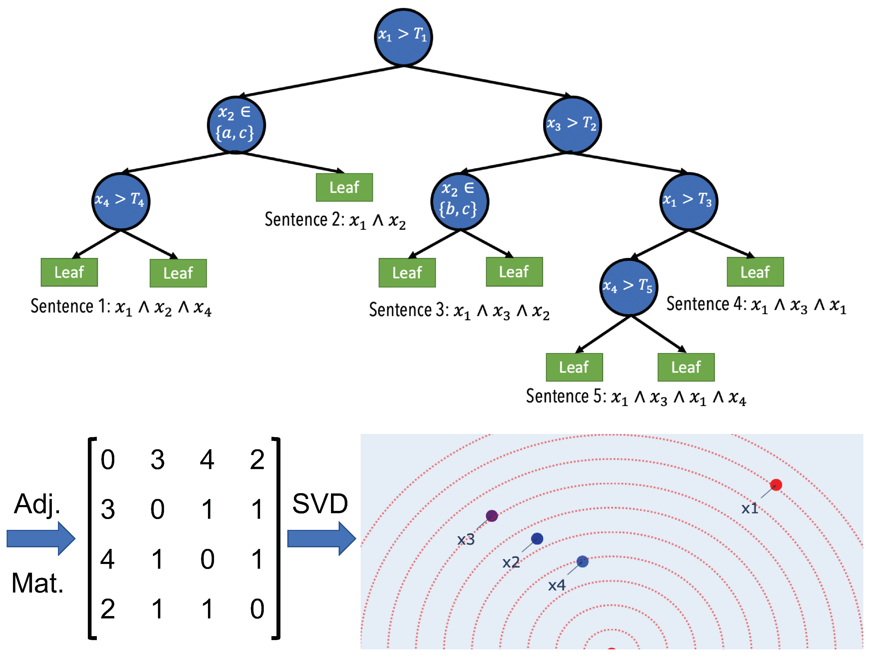
2.1. Semantic Embedding

Our objective is to compute an embedding for each feature that contains both importance and semantic information. Inspired by word embeddings in Natural Language Processing (NLP), we are looking for a continuous dense representation of features that contains semantic information. We define two features to be semantically similar if they are exchangeable with respect to the feature interactions that determine the model’s predictions. We want this similarity to be reflected in the cosine similarity of their embeddings. Similar to the common objective in NLP, enforcing exchangeability in the context of other features will make it possible to find such a representation. In NLP, one simple embedding technique common in NLP tasks is using the co-occurrence of words in the vocabulary [48,49,50]. The intuition is that if two words are semantically similar, in a large enough corpora of sentences, their (normalized) co-occurrence frequency with other words will be similar. For a large dictionary size, in order to have a low-dimensional word embedding, Singular Value Decomposition (SVD) dimensionality reduction is applied to the co-occurrence matrix.
There are some problems and limitations with directly applying the idea of word-vectors to features. First of all, unlike NLP where computing word embeddings is possible due to virtually unlimited supply of grammatically structured text data, in tabular data, co-occurrence of features in is not clearly defined and there is no corpus of structured co-occurrence of features. Luckily, in addition to their strong predictive performance, tree-based models naturally provide us with a structured co-occurrence of features. As shown in Figure 1, a tree contains a number of decision paths where each path is a conjunction of binary conditions on a number of features. Secondly, considering a group of words with similar meanings, each word has a non-zero chance of appearing in a sentence while in a decision tree, among a group of similar features, only the most predictive feature will be chosen at its respective split. For example, consider a salary prediction task where there are two features with similar information about the outcome: earned degree (categorical) and number of years at college (numerical). Assuming that earned degree is a better predictor, in a given split of the tree (e.g., in a decision path that also contains age and marital status features), it will always be chosen over number of years at college. As a result, it is not possible to extract the co-occurrence of number of years at college with other features and to observe its exchangeability with earned degree. The solution is to enforce a non-zero chance of occurrence to all features in a given decision path. The solution is to train a large ensemble of trees where each tree is only given a random subset of features (i.e., a random forest). This is the same as using a Random Forest model.

2.2. Feature Importance

In natural language, word embeddings are computed with a normalization constraint so that only the semantic information is preserved in the embedding angles [51,52]. Our goal, however, is to preserve both importance and semantic information. After extracting the sentences from the trained random forest, a feature’s co-occurrence with other features is a direct indicator of how many times it was chosen in a split. For example, between two similar features, the less important one will only be chosen in a split if the other feature is not present. Therefore, although the normalized co-occurrence frequency of both features is similar, the absolute co-occurrence of the less informative feature will be smaller. Thus, the Feature Vectors algorithm computes word embeddings using the counts of co-occurrence.

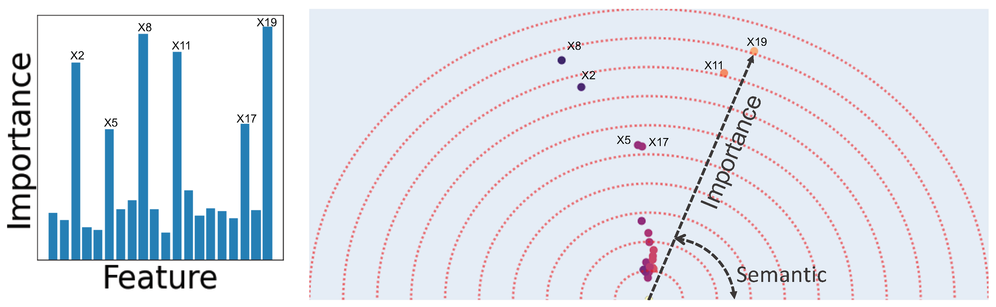
2.3. Human-Understandable Visualization

The last desired property is to have a human-understandable visualization. After computing the co-occurrence matrix of features, to be able to visualize the features in an intuitive fashion, we reduce the dimensionality of word embeddings to two. One possible drawback is that a two dimensional embedding might lose some of the information from the feature co-occurrence pattern. In practice, for all real-world datasets that we examined, between 80 % to 99 % of the co-occurrence matrix’s variance is explained by the first two components.

2.4. Feature Vectors Algorithm

The pseudo-code in Algorithm 1 describes the Feature Vectors algorithm’s steps. Let us discuss the computational overhead that the Feature Vectors algorithm has over training an ensemble of trees. After all the trees have been trained, the complexity of the algorithm depends on d the number of features, R the total number of sentences (i.e., number of all decision paths in all trees), and w the sliding window size. Creating the co-occurrence matrix requires O ( R × w ) operations (with the underlining assumption that the trees are not too deep, otherwise you should multiply by depth). Computing the SVD-decomposition requires O ( d 3 ) operations. As the number of sentences is usually fixed on the order of 10 5 10 6 , the algorithm’s speed is bottlenecked by the dataset dimensionality for datasets with 100 or more features. Therefore, the algorithm is efficient to run for datasets that do not have a very large number of features. Using the truncated SVD implementation of the Scikit Learn [53] library, on a workstation with eight Intel(R) Core(TM) i9-9960X cpus, the algorithm takes about thirty seconds to run for a dataset with 50,000 features.
Algorithm 1 Feature Vectors
1:
Input: A dataset tabular X with n data points (rows) and d categorical or numerical features (columns), n prediction targets y (categorical for classification and numerical for regression)
2:
Hyperparameters: Number of rules R (number of total decision paths in all of the trees), co-occurrence sliding window size w used for counting the co-occurrence of features that appear in a sentence
3:
Output: Feature embeddings v 1 , , v d R 2 .
4:
Initialization: Set of sentences S = { }
5:
while | S | < R do
6:
   Train a decision tree on ( X , y ) . The training is done such that at each split of the tree, only a random subset of size d of features is considered rather than the whole feature set.
7:
    s t = Set of all decision paths in the tree. A sentence or a decision path is the list of features that are used at consecutive splits starting from the root of the tree and ending at a leaf. A Tree with M leaves contains M decision paths.
8:
    S = S s t
9:
Initialization: Co-occurrence matrix M R d × d . Set all elements of M to be zero.
10:
for s S do
11:
   Slide a window of size w on s and for each pair of features x i and x j that are in the window, increase M i j and M j i by one.
12:
Apply 2 d truncated SVD on M: M T R d × 2
13:
M T = v 1 T v d T Each row is the embedding vector of one of the features.

2.5. Comparison with Existing Methods

Existing global interpretability methods like gini importance, SHAP [30], and permutation importance [20] will only provide scalar values for each feature and the result is similar to Figure 2’s bar chart. In comparison, the output of feature vectors, while preserving the importance information, also shows the groups of features that are semantically similar in the eyes of the model.
Unlike Feature Vectors that computes the feature embeddings using the input-output relationship, an alternative approach is to find the feature-importance (size) and semantic similarity (angle) separately. We can use any existing importance method to find the size and then, if all the features are numerical, we can use the features’ covariance matrix (instead of feature co-occurrence) to compute the semantic similarity of features. As tabular data is usually a mix of categorical and numerical variables, point-biserial correlation can be used to mitigate the issue of having mixed-type variables. We show the possible drawback of such an approach using an example in Figure 2. We create a synthetic dataset where the 20 features are sampled from independent normal distributions. The label is assigned using a set of logical expressions from binary thresholds applied to the first 6 input features, e.g., ( x 1 > 2 x 2 < 3 ) x 1 > 0 where for each true expression, the chance of y = 1 increases. Only 6 features are present in the expressions and we divide them into three pairs. The logical expressions are created such that each group of paired features are interchangeable, that is, for every expression that contains one of the features, similar expressions that contain other features of that group exist. In other words, the two features in a group are semantically similar. Figure 2 shows that our method perfectly discovers the pairs of semantically similar features while any covariance-based method will fail as the features are independent.

3. Experiments and Results

In this section, we first show a few examples of Feature Vectors implementation on widely used tabular datasets to show the usefulness of information provided by our method. The second set of experiments aims to show that the fature-importance measure provided by this method are objectively valid. We finally use the notion of Knockoff features [54] to examine the information provided by the angle. For all experiments, we use cross-validation for selecting the depth of trees. We empirically observe by setting R = 100,000 (number of rules), the computed feature embeddings become stable across multiple runs. We also set the window size to w = 3 .

3.1. Easy to Implement

The implementation of Feature Vectors is available as a Python package and can be accessed from https://github.com/featurevec/featurevec (accessed on 18 October 2021). This tool is easy to use in general, and seamlessly integrates with Scikit-Learn’s [53] tree-based models in a few lines of code:
1from featurevec import FeatureVec
2from sklearn.ensemble import RandomForestClassifier
3X, y, feature_names = data_loader ()
4predictor = RandomForestClassifier ().fit (X, y)
5fv = FeatureVec (
6  mode = ’classify ’,
7  feature_names = feature_names,
8  tree_generator = predictor
9  )
10fv.fit (X, y)
11fv.plot ()

3.2. Case Studies on Real-World Datasets

We first apply the Feature Vectors method to three real-world datasets and discuss the explanation provided by the algorithm. Feature-vectors outputs are shown in Figure 3 for three tabular datasets:
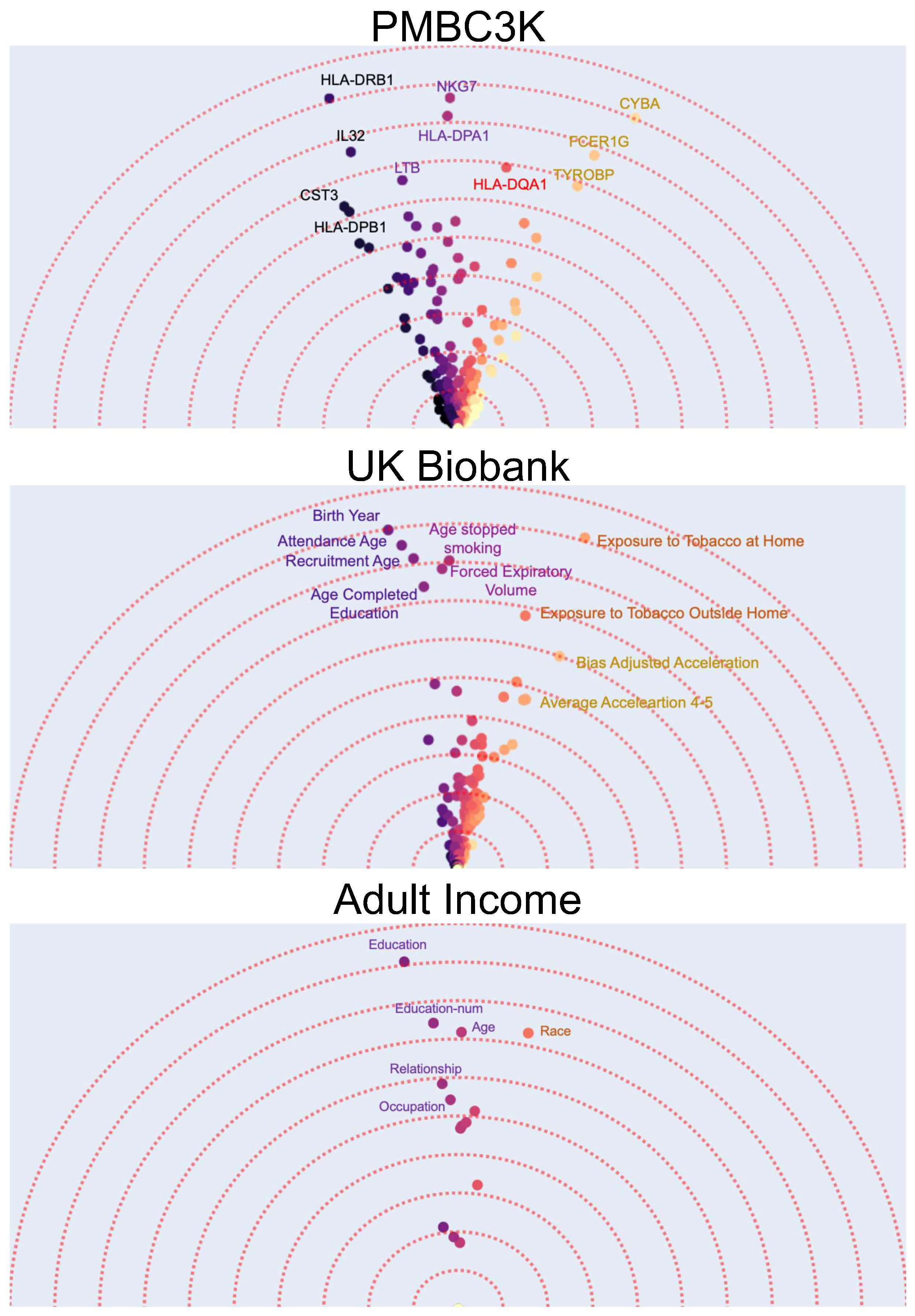
  • The first dataset contains gene expression of around 1800 genes for 3000 peripheral blood mononuclear cells (PBMCs) from a healthy donor [55] i.e., each data point is a single cell and has 1800 numerical features. Using K-means algorithm, the data points are clustered into eight different groups. The task is a binary prediction with a goal to predict whether a given cell is normal (i.e., belongs to the largest cluster) or not. Using interpretability methods after training a binary classifier model on this dataset can allow us to find the important (e.g., top-10) features (i.e., gene expressions). These could potentially be used as “marker genes” that determine if a cell is normal or not. Using Feature Vectors, however, in addition to finding the marker genes by their importance, we have a more detailed interpretation of how the different marker genes interact in determining if a cell is normal (Figure 3a). A gene can be characterized as important not just by the magnitude of it’s contribution but also by it’s uniqueness. In this case, it can be observed that the effects of marker genes can be clustered into four major groups with similar genes. Furthermore, although the HLA-DQA1 gene is not among the top-5 genes with the highest feature-importance, it is an important marker as it is unique and does not have any other similar genes to it.
  • As our second dataset we use the UK Biobank dataset [56]. The UK Biobank dataset has comprehensive phenotype and genotype information of 500,000 individuals in the UK. This information includes among others gender, age, medical history, diet, etc. Using the original dataset and specifically the medical history data, we create a new dataset by selecting the subset of individuals (data points) that are later diagnosed with lung cancer and randomly selecting another equally large subset of individuals that do not get lung cancer. The result is a new binary classification dataset where the task is to predict whether a person will be diagnosed with lung cancer. We use the 341 phenotypic features that have the least number of missing values in the dataset. It is known that a number of phenotypic factors can be used to predict lung cancer but it might not be clear whether they all carry similar information. Therefore, after applying the Feature Vectors algorithm to this dataset, we can investigate the high importance features and how they cluster together. Figure 3 shows that there are three main groups of phenotypic features. A group of features that are related to age and how much time has passed since the person stopped smoking, a group of features that show the overall exposure to tobacco, and a group of features that describe the activity level.
  • As out last dataset, we choose the classic and frequently used adult income prediction dataset from the UCI repository of machine learning datasets [57,58]. This dataset is extracted from census data and contains demographical information (marital status, education, etc.) of around 50 thousand individuals. The task is to predict whether their income is above 50 thousand dollars. After applying the Feature Vectors algorithm to this dataset, we can see that education (including education-num), age, and race are the best predictors. An interesting observation is that education as a categorical feature and education-num as a numerical feature are semantically similar while education is a better predictor. This is expected as the number of years of education is an approximate indicator of education level.

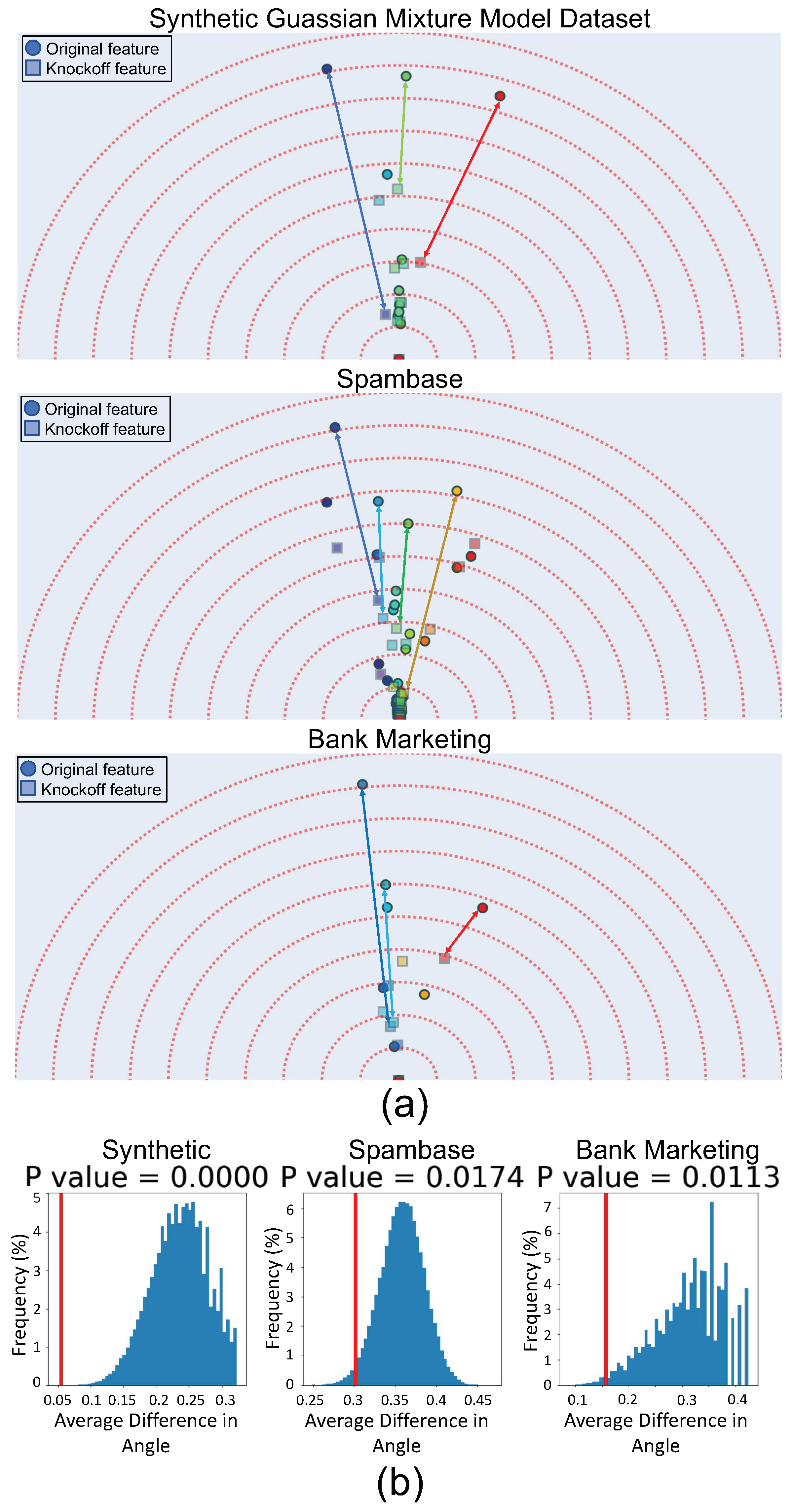
3.3. Validating Feature Vector Angles Using Knockoffs

Our next experiment seeks to objectively verify the angle as a valid similarity measure. We find the notion of “Knockoff” features the best tool for examination. In short, for a given feature, its knockoff is a fake feature that has perfectly similar interactions with all other features in the data. However, it only has predictive power if the original feature is removed, i.e., it is conditionally independent from the outcome. Therefore, in the Feature Vectors plot, if the original feature has predictive power, we expect a feature and it’s knockoff have similar angles with different magnitudes. A formal definition is as follows: for a d-dimensional random variable X, its knockoff X ˜ is a random variable that satisfies:
  • Conditional independence from outcome: X ˜ Y | X
  • Exchangeability S { 1 , , d }
    [ X , X ˜ ] s w a p ( S ) = d [ X , X ˜ ]
where = d means equality in distribution and [ X , X ˜ ] s w a p ( S ) means swapping the original and knockoff features in S. The exchangeability condition results in perfect semantic similarity of a feature and its knockoff while the independence condition means that if an original feature has predictive importance (i.e., it is not null: X j Y | X j ), its knockoff will have a smaller importance.
Figure 4 shows the Feature Vectors output for three datasets where the features and their knockoffs are present (the models is trained on the concatenation of [X, X ˜ ]). The difficulty with knockoffs is that generating them for an arbitrary distribution of data is not possible. In [59] it was shown that if the distribution of X is a mixture of Gaussians, one can sample the knockoffs. Therefore, our first dataset is a synthetic 20-dimensional mixture of three Gaussians, where only the first three features are non-null (predictive of the outcome). As expected, in Figure 4a, we observe that the features (circles) and their knockoff (squares) have similar angles. Additionally, we can see that for non-null features, the knockoffs have a smaller importance while for other features the knockoff and the original feature have similar feature vectors. For the other two real-world datasets, the validity of the generated knockoffs depends on the validity of the Gaussian Mixture Model (GMM) assumption. Following [59], we fit a GMM model to the data. We can see in Figure 4a that the features and their knockoffs have similar angles. In addition to the subjective observation, we perform a permutation test in Figure 4b to measure the semantic similarity of original and knockoff features. The null hypothesis is that the average difference in the angle between features and their knockoffs is not different from the average difference in a random pairing of features. As expected, the hypothesis is rejected with p-values close to 0.01 .

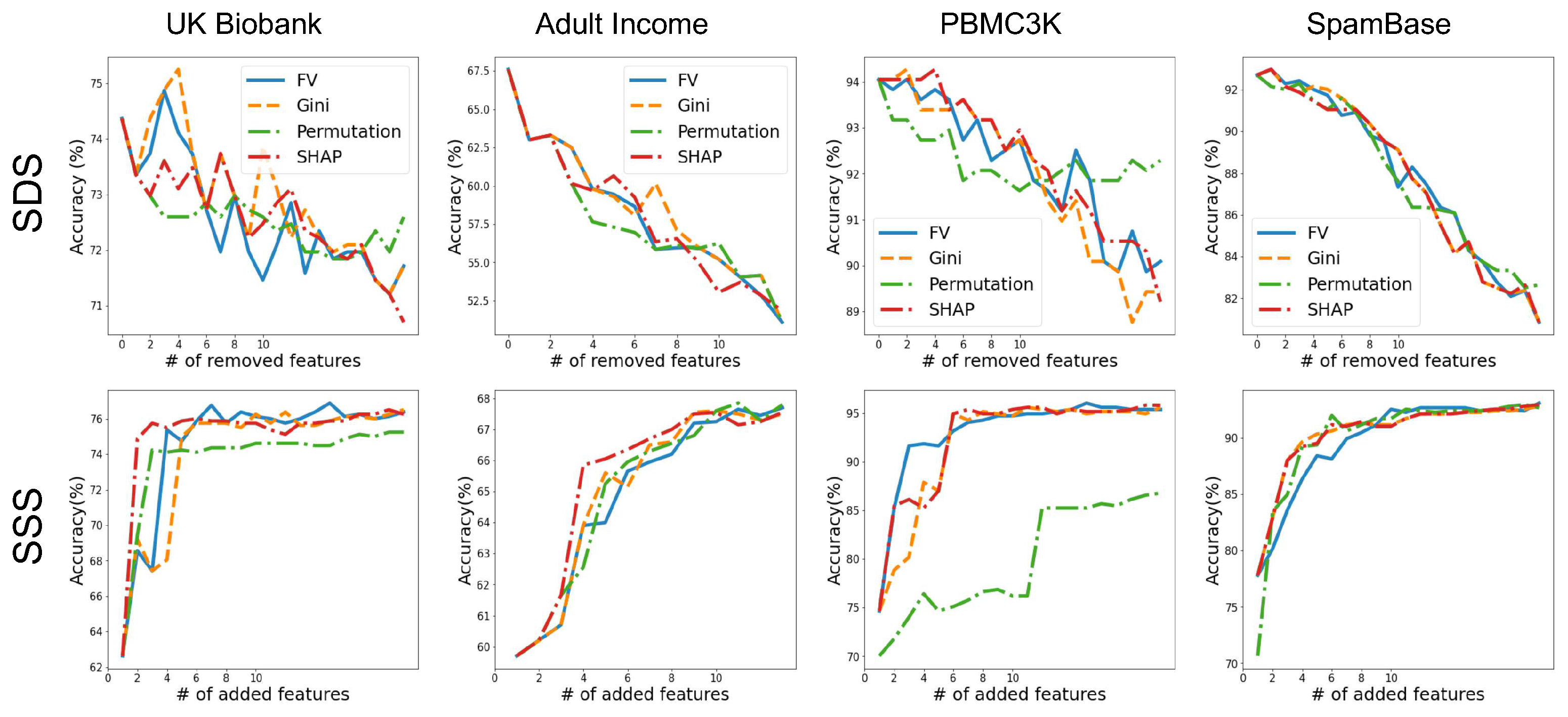
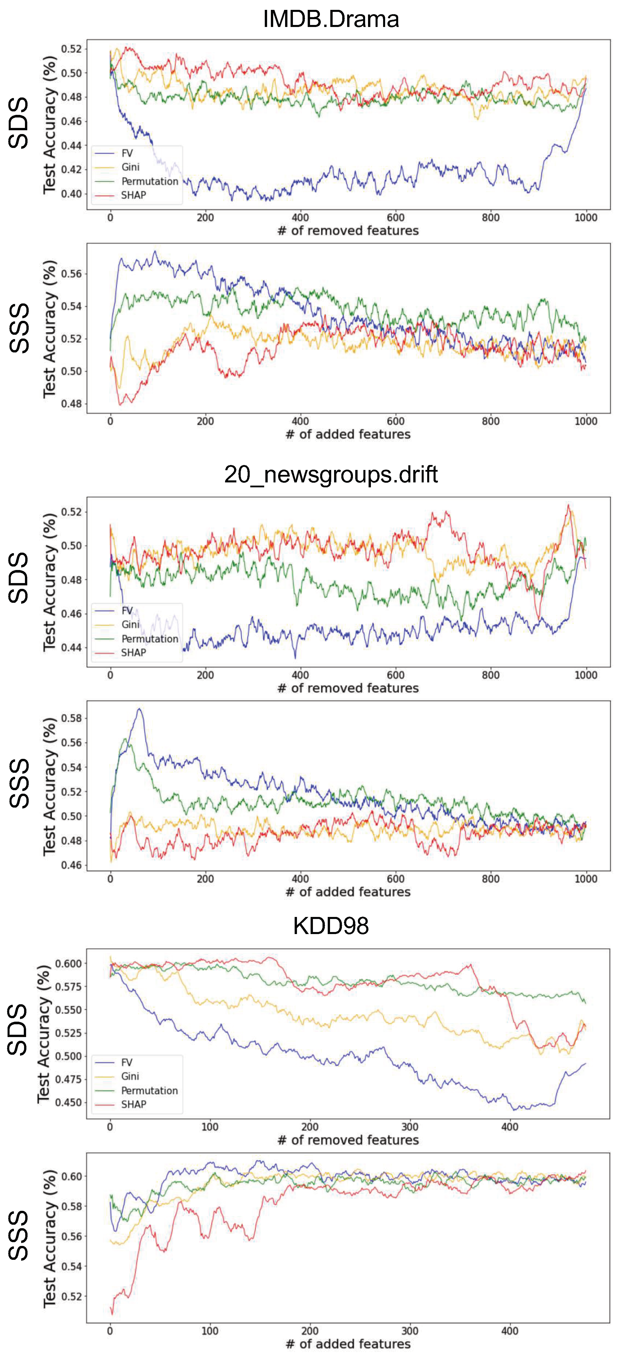
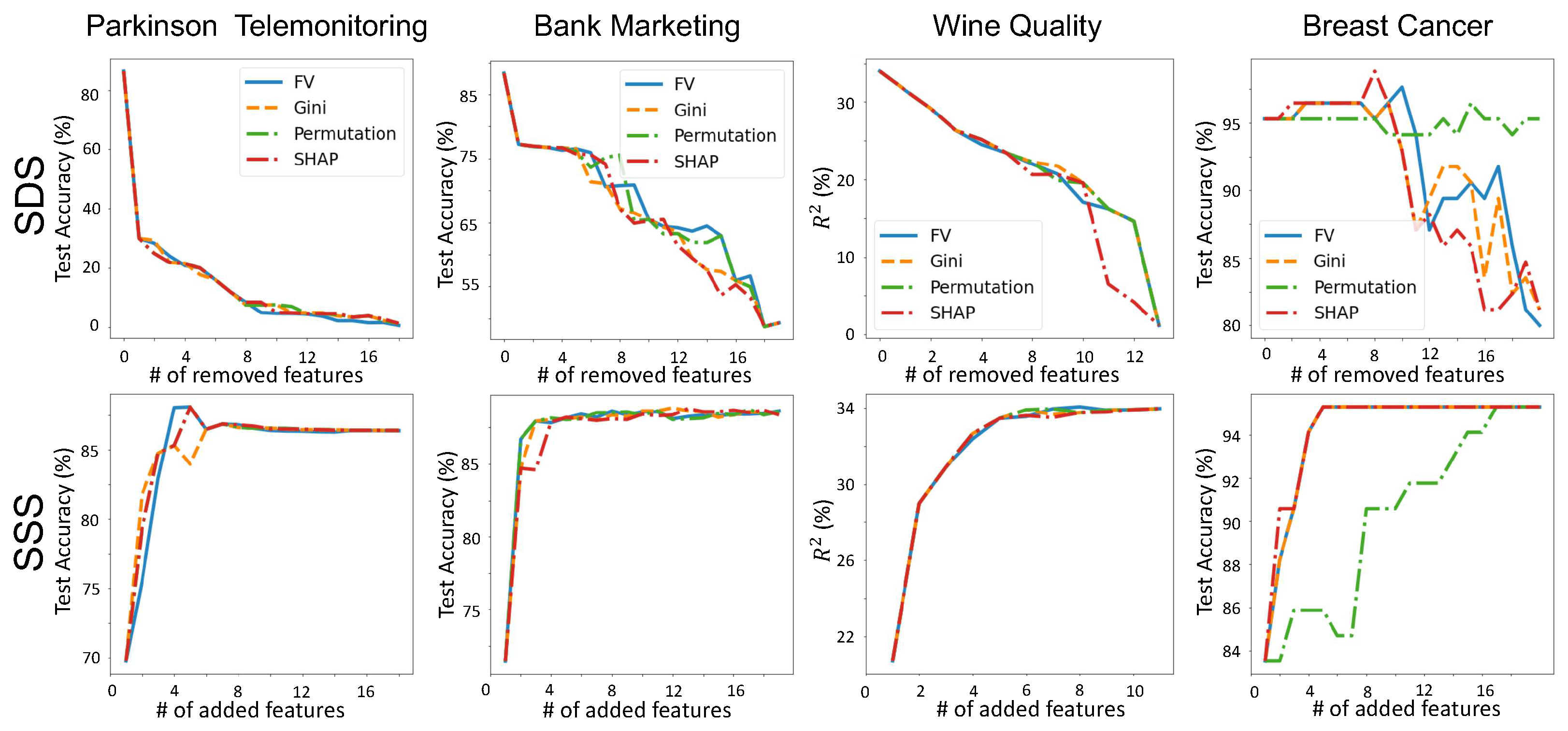
3.4. Validating Feature-Importance Scores

We conduct quantitative experiments to verify the feature-importance generated by the Feature Vectors visualization. There exist various objective metrics for measuring the goodness of global feature-importance methods and following existing work [19,60], we will focus on two intuitive and widely used metrics:
  • Smallest Destroying Subset (SDS)—Smallest subset of features that by removing them an accurate model cannot be trained.
  • Smallest Sufficient Subset (SSS)—Smallest subset of features that are sufficient for training an accurate model.
To measure SSS (SDS), we start removing (adding) features from the most important to the least important one by one (based on each method’s importance scores) and each time train a new model and measure its performance. Figure 5 shows the performance of Feature Vectors compared to three other famous global interpretability methods on four UCI ML repository datasets [57] (More examples are provided in Appendix B). Other methods are: (1) Gini Importance score which computes the number of times each feature has been used in a split proportional to the number of samples it splits. (2) Permutation Importance [20] which removes features one by one by permuting its value in different data points and computes the drop in model’s performance. (3) TreeSHAP [37], which models the features as players in a cooperative game and computes the contribution of each feature to the collaboration using the notion of Shapley value. We can see that Feature Vectors has a comparable performance to the other three and as expected, correlates very well with the Gini importance method. To showcase the advantage of the Feature Vectors algorithm to other methods, we run the same experiment but for three high-dimensional datasets (results are shown in Appendix C). This shows that as the dimension of the dataset increases, Feature Vectors’ advantage becomes more clear.
All in all, while Feature Vectors provides feature-importance scores that are as good as or better than other existing interpretability methods, it provides semantic information of the features.
One important question is how stable these results are across different runs of the Feature Vectors algorithm. To answer this question, we take 54 tabular datasets from the Open ML repository [61] (We have provided Feature Vectors visualization of these tabular datasets along with their names here: https://github.com/featurevec/featurevec/tree/main/example/plots/OpenML, accessed on 18 October 2021) and for each dataset, we train a new ensemble of trees and compute the Feature-Vectors 10 different times. To have a single performance metric, for each run we compute the area under the SSS curve. We realize that among all of the datasets, there is at most a 1 % difference (on average 0.5 % difference) between the largest and smallest area under curve of the different runs. This shows that the Feature Vectors algorithm’s performance is stable across different runs in the sense that the ordering of the features’ importance is preserved (on average, Spearman’s Rank Correlation of the importance scores of features in a dataset across different runs is 0.984 ). We could extend the stability analysis to the changes in the embedding vector itself. On average, the relative difference between maximum and minimum 2 norm of a feature’s embedding vector across different runs is 15.5 % . The maximum angular difference between the same feature’s embedding vector in 10 runs is on average 5.2 . This shows that the visualized information is also stable across different runs.

4. Discussion and Conclusions

We introduce Feature Vectors, a global interpretability method for tabular ML. Feature Vectors takes a tabular dataset as an input and outputs a visualization of features where each feature is shown by its two dimensional embedding (see Appendix A). The embeddings explain two main aspects of the data: (1) the magnitude of the embedding gives how the importance of the feature to the predictive power of the model. (2) The direction of the corresponding feature shows how semantically similar or dissimilar it is to other features. Semantic similarity is defined as an interpretation tool where two features that are semantically similar have similar interactions with other features in predicting the outcome. Through extensive quantitative and qualitative experiments, we show that using Feature Vectors can help users have a better understanding of the model while not losing any information compared to other existing methods. This work opens a new window towards creating better interpretability tools for tabular data and using the element of visualization as a tool for intuitive explanations of feature interactions. One interesting future direction is to extend this global interpretability method for local explainability as well. Feature Vectors is intrinsically limited to the tree-based models that randomly select subsets of features (e.g., random forests) and an important future direction is to extend the notion of feature semantics to other models that are used for tabular data.

Author Contributions

Initial study concept and design: A.G. and J.Y.Z.; Implementation and model training: A.G. and D.B.; Analysis and interpretation of data: A.G., D.B. and J.Y.Z.; Drafting of the paper: A.G., D.B., M.I., Y.D. and J.Y.Z.; Critical revision of the manuscript for important intellectual content: D.B., M.I., Y.D. and J.Y.Z. All authors have read and agreed to the published version of the manuscript.

Funding

This research received no external funding.

Institutional Review Board Statement

Not applicable.

Informed Consent Statement

Not applicable.

Data Availability Statement

All of the utilized datasets are publicly availabe. The implementation can be found at https://github.com/featurevec/featurevec (accessed on 18 October 2021).

Conflicts of Interest

The authors declare no conflict of interest.

Appendix A. Two Dimensional Embeddings Are Sufficient

Table A1 shows the percentage of explained variance of the co-occurrence matrix using the 2-dimensional Feature Vectors embedding.
Table A1. Explained Variance Ratio.
DatasetExplained Variance (%)
UK Biobank Lung Cancer Prediction81
PBMC3k85
Adult Income92
Spambase86
Bank Marketing98
Parkinson Telemonitoring99
Wine Quality98
Breast Cancer87

Appendix B. Comparing Feature-Importance Methods

In Figure A1, we compare the feature importance scores of different methods using the SSS and SDS metrics for four more datasets.
Figure A1. Importance scores comparison. Feature vectors importance scores are compared with Gini, Permutation, and SHAP global importance methods. The first row shows the SDS results were we remove features from the most important and train a new model each time and report its test performance. The bottom row shows the SSS results were we add the features with the order of importance and train a new model and reports its test performance. We can see that the Feature Vectors has similar performance to other methods.
Information 13 00015 g0a1

Appendix C. Comparing Feature-Importance Methods in High-Dimensional Setting

In Figure A2, we compare the feature importance scores of different methods using the SSS and SDS metrics for four dataset with high dimensionality from the Open ML reopository. Compared to other datasets, the advantage of the FV algorithm is more clear in these results.
Figure A2. Importance scores comparison. Feature vectors importance scores are compared with Gini, Permutation, and SHAP global importance methods for high-dimensional datasets. The first row shows the SDS results (the lower the better) where we remove features from the most important and train a new model each time and report its test performance. The bottom row shows the SSS results (the higher the better) were we add the features with the order of importance and train a new model and reports its test performance. We can see that the Feature Vectors has better performance to other methods. (For better visualization, the plots are smoothed with a moving average of size 5).
Information 13 00015 g0a2

References

  1. Ouyang, D.; He, B.; Ghorbani, A.; Yuan, N.; Ebinger, J.; Langlotz, C.P.; Heidenreich, P.A.; Harrington, R.A.; Liang, D.H.; Ashley, E.A.; et al. Video-based AI for beat-to-beat assessment of cardiac function. Nature 2020, 580, 252–256. [Google Scholar] [CrossRef] [PubMed]
  2. Ghorbani, A.; Ouyang, D.; Abid, A.; He, B.; Chen, J.H.; Harrington, R.A.; Liang, D.H.; Ashley, E.A.; Zou, J.Y. Deep learning interpretation of echocardiograms. NPJ Digit. Med. 2020, 3, 1–10. [Google Scholar] [CrossRef] [Green Version]
  3. Esteva, A.; Kuprel, B.; Novoa, R.A.; Ko, J.; Swetter, S.M.; Blau, H.M.; Thrun, S. Dermatologist-level classification of skin cancer with deep neural networks. Nature 2017, 542, 115–118. [Google Scholar] [CrossRef]
  4. Dixon, M.F.; Halperin, I.; Bilokon, P. Machine Learning in Finance; Springer: Berlin, Germany, 2020. [Google Scholar]
  5. Heaton, J.B.; Polson, N.G.; Witte, J.H. Deep learning for finance: Deep portfolios. Appl. Stoch. Model. Bus. Ind. 2017, 33, 3–12. [Google Scholar] [CrossRef]
  6. Goodman, B.; Flaxman, S. European Union regulations on algorithmic decision-making and a “right to explanation”. AI Mag. 2017, 38, 50–57. [Google Scholar] [CrossRef] [Green Version]
  7. Jouppi, N.P.; Young, C.; Patil, N.; Patterson, D.; Agrawal, G.; Bajwa, R.; Bates, S.; Bhatia, S.; Boden, N.; Borchers, A.; et al. In-datacenter performance analysis of a tensor processing unit. In Proceedings of the 44th Annual International Symposium on Computer Architecture, New York, NY, USA, 24–28 June 2017; pp. 1–12. [Google Scholar]
  8. Arik, S.O.; Pfister, T. Tabnet: Attentive interpretable tabular learning. arXiv 2019, arXiv:1908.07442. [Google Scholar]
  9. Yang, Y.; Morillo, I.G.; Hospedales, T.M. Deep neural decision trees. arXiv 2018, arXiv:1806.06988. [Google Scholar]
  10. Erickson, N.; Mueller, J.; Shirkov, A.; Zhang, H.; Larroy, P.; Li, M.; Smola, A. Autogluon-tabular: Robust and accurate automl for structured data. arXiv 2020, arXiv:2003.06505. [Google Scholar]
  11. Carvalho, D.V.; Pereira, E.M.; Cardoso, J.S. Machine learning interpretability: A survey on methods and metrics. Electronics 2019, 8, 832. [Google Scholar] [CrossRef] [Green Version]
  12. Ribeiro, M.T.; Singh, S.; Guestrin, C. Model-agnostic interpretability of machine learning. arXiv 2016, arXiv:1606.05386. [Google Scholar]
  13. Sundararajan, M.; Taly, A.; Yan, Q. Axiomatic attribution for deep networks. In Proceedings of the International Conference on Machine Learning, PMLR, Sydney, Australia, 6–11 August 2017; pp. 3319–3328. [Google Scholar]
  14. Smilkov, D.; Thorat, N.; Kim, B.; Viégas, F.; Wattenberg, M. Smoothgrad: Removing noise by adding noise. arXiv 2017, arXiv:1706.03825. [Google Scholar]
  15. Poursabzi-Sangdeh, F.; Goldstein, D.G.; Hofman, J.M.; Wortman Vaughan, J.W.; Wallach, H. Manipulating and measuring model interpretability. In Proceedings of the 2021 CHI Conference on Human Factors in Computing Systems, Yokohama, Japan, 8–13 May 2021; pp. 1–52. [Google Scholar]
  16. Kim, B.; Wattenberg, M.; Gilmer, J.; Cai, C.; Wexler, J.; Viegas, F.; et al. Interpretability beyond feature attribution: Quantitative testing with concept activation vectors (tcav). In Proceedings of the International Conference on Machine Learning, PMLR, Stockholm, Sweden, 10–15 July 2018; pp. 2668–2677. [Google Scholar]
  17. Zhou, B.; Sun, Y.; Bau, D.; Torralba, A. Interpretable basis decomposition for visual explanation. In Proceedings of the European Conference on Computer Vision (ECCV), Munich, Germany, 8–14 September 2018; pp. 119–134. [Google Scholar]
  18. Bouchacourt, D.; Denoyer, L. Educe: Explaining model decisions through unsupervised concepts extraction. arXiv 2019, arXiv:1905.11852. [Google Scholar]
  19. Ghorbani, A.; Wexler, J.; Zou, J.Y.; Kim, B. Towards Automatic Concept-based Explanations. Adv. Neural Inf. Process. Syst. 2019, 32, 9277–9286. [Google Scholar]
  20. Breiman, L. Random forests. Mach. Learn. 2001, 45, 5–32. [Google Scholar] [CrossRef] [Green Version]
  21. Chen, T.; Guestrin, C. Xgboost: A scalable tree boosting system. In Proceedings of the 22nd ACM Sigkdd International Conference on Knowledge Discovery and Data Mining, San Francisco, CA, USA, 13–17 August 2016; pp. 785–794. [Google Scholar]
  22. Geurts, P.; Ernst, D.; Wehenkel, L. Extremely randomized trees. Mach. Learn. 2006, 63, 3–42. [Google Scholar] [CrossRef] [Green Version]
  23. Ke, G.; Meng, Q.; Finley, T.; Wang, T.; Chen, W.; Ma, W.; Ye, Q.; Liu, T.Y. Lightgbm: A highly efficient gradient boosting decision tree. Adv. Neural Inf. Process. Syst. 2017, 30, 3146–3154. [Google Scholar]
  24. Prokhorenkova, L.; Gusev, G.; Vorobev, A.; Dorogush, A.V.; Gulin, A. CatBoost: Unbiased boosting with categorical features. Adv. Neural Inf. Process. Syst. 2018, 31. [Google Scholar]
  25. Loh, W.Y. Classification and regression trees. Wiley Interdiscip. Rev. Data Min. Knowl. Discov. 2011, 1, 14–23. [Google Scholar] [CrossRef]
  26. Friedman, J.; Hastie, T.; Tibshirani, R. The Elements of Statistical Learning; Springer Series in Statistics New York; Springer: New York, NY, USA, 2001; Volume 1. [Google Scholar]
  27. Sandri, M.; Zuccolotto, P. A bias correction algorithm for the Gini variable importance measure in classification trees. J. Comput. Graph. Stat. 2008, 17, 611–628. [Google Scholar] [CrossRef]
  28. Auret, L.; Aldrich, C. Empirical comparison of tree ensemble variable importance measures. Chemom. Intell. Lab. Syst. 2011, 105, 157–170. [Google Scholar] [CrossRef]
  29. Strobl, C.; Boulesteix, A.L.; Kneib, T.; Augustin, T.; Zeileis, A. Conditional variable importance for random forests. BMC Bioinform. 2008, 9, 1–11. [Google Scholar] [CrossRef] [PubMed] [Green Version]
  30. Lundberg, S.M.; Lee, S.I. A unified approach to interpreting model predictions. In Proceedings of the 31st International Conference on Neural Information Processing Systems, Long Beach, CA, USA, 4–9 December 2017; pp. 4768–4777. [Google Scholar]
  31. Ribeiro, M.T.; Singh, S.; Guestrin, C. “Why should i trust you?” Explaining the predictions of any classifier. In Proceedings of the 22nd ACM SIGKDD International Conference on Knowledge Discovery and Data Mining, San Fransisco, CA, USA, 13–17 August 2016; pp. 1135–1144. [Google Scholar]
  32. Ribeiro, M.T.; Singh, S.; Guestrin, C. Anchors: High-precision model-agnostic explanations. In Proceedings of the AAAI Conference on Artificial Intelligence, New Orleans, LA, USA, 2–7 February 2018; Volume 32. [Google Scholar]
  33. Chen, J.; Song, L.; Wainwright, M.; Jordan, M. Learning to explain: An information-theoretic perspective on model interpretation. In Proceedings of the International Conference on Machine Learning, PMLR, Stockholm, Sweden, 10–15 July 2018; pp. 883–892. [Google Scholar]
  34. Ancona, M.; Ceolini, E.; Öztireli, C.; Gross, M. Towards better understanding of gradient-based attribution methods for Deep Neural Networks. In Proceedings of the 6th International Conference on Learning Representations, Vancouver, BC, Canada, 30 April– 3 May 2018. [Google Scholar]
  35. Simonyan, K.; Vedaldi, A.; Zisserman, A. Deep inside convolutional networks: Visualising image classification models and saliency maps. arXiv 2013, arXiv:1312.6034. [Google Scholar]
  36. Selvaraju, R.R.; Cogswell, M.; Das, A.; Vedantam, R.; Parikh, D.; Batra, D. Grad-cam: Visual explanations from deep networks via gradient-based localization. In Proceedings of the IEEE International Conference on Computer Vision, Venice, Italy, 22–29 October 2017; pp. 618–626. [Google Scholar]
  37. Lundberg, S.M.; Erion, G.G.; Lee, S.I. Consistent individualized feature attribution for tree ensembles. arXiv 2018, arXiv:1802.03888. [Google Scholar]
  38. Tsang, M.; Rambhatla, S.; Liu, Y. How does this interaction affect me? Interpretable attribution for feature interactions. arXiv 2020, arXiv:2006.10965. [Google Scholar]
  39. Sundararajan, M.; Dhamdhere, K.; Agarwal, A. The Shapley Taylor Interaction Index. In Proceedings of the International Conference on Machine Learning, PMLR, Vienna, Austria, 12–18 July 2020; pp. 9259–9268. [Google Scholar]
  40. Janizek, J.D.; Sturmfels, P.; Lee, S.I. Explaining explanations: Axiomatic feature interactions for deep networks. J. Mach. Learn. Res. 2021, 22, 1–54. [Google Scholar]
  41. Friedman, J.H.; Popescu, B.E.; et al. Predictive learning via rule ensembles. Ann. Appl. Stat. 2008, 2, 916–954. [Google Scholar] [CrossRef]
  42. Hooker, G. Discovering additive structure in black box functions. In Proceedings of the Tenth ACM SIGKDD International Conference on Knowledge Discovery and Data Mining, Seattle, WA, USA, 22–25 August 2004; pp. 575–580. [Google Scholar]
  43. Greenwell, B.M.; Boehmke, B.C.; McCarthy, A.J. A simple and effective model-based variable importance measure. arXiv 2018, arXiv:1805.04755. [Google Scholar]
  44. Basu, S.; Kumbier, K.; Brown, J.B.; Yu, B. Iterative random forests to discover predictive and stable high-order interactions. Proc. Natl. Acad. Sci. USA 2018, 115, 1943–1948. [Google Scholar] [CrossRef] [Green Version]
  45. Apley, D.W.; Zhu, J. Visualizing the effects of predictor variables in black box supervised learning models. J. R. Stat. Soc. Ser. B Stat. Methodol. 2020, 82, 1059–1086. [Google Scholar] [CrossRef]
  46. Goldstein, A.; Kapelner, A.; Bleich, J.; Pitkin, E. Peeking inside the black box: Visualizing statistical learning with plots of individual conditional expectation. J. Comput. Graph. Stat. 2015, 24, 44–65. [Google Scholar] [CrossRef]
  47. Zhao, Q.; Hastie, T. Causal interpretations of black-box models. J. Bus. Econ. Stat. 2021, 39, 272–281. [Google Scholar] [CrossRef] [PubMed]
  48. Bengio, Y.; Ducharme, R.; Vincent, P.; Janvin, C. A neural probabilistic language model. J. Mach. Learn. Res. 2003, 3, 1137–1155. [Google Scholar]
  49. Collobert, R.; Weston, J. A unified architecture for natural language processing: Deep neural networks with multitask learning. In Proceedings of the 25th International Conference on Machine Learning, Helsinki, Finland, 5–9 July 2008; pp. 160–167. [Google Scholar]
  50. Mikolov, T.; Sutskever, I.; Chen, K.; Corrado, G.S.; Dean, J. Distributed representations of words and phrases and their compositionality. Adv. Neural Inf. Process. Syst. 2013, 26, 3111–3119. [Google Scholar]
  51. Levy, O.; Goldberg, Y.; Dagan, I. Improving distributional similarity with lessons learned from word embeddings. Trans. Assoc. Comput. Linguist. 2015, 3, 211–225. [Google Scholar] [CrossRef]
  52. Wilson, B.J.; Schakel, A.M. Controlled experiments for word embeddings. arXiv 2015, arXiv:1510.02675. [Google Scholar]
  53. Pedregosa, F.; Varoquaux, G.; Gramfort, A.; Michel, V.; Thirion, B.; Grisel, O.; Blondel, M.; Prettenhofer, P.; Weiss, R.; Dubourg, V.; et al. Scikit-learn: Machine Learning in Python. J. Mach. Learn. Res. 2011, 12, 2825–2830. [Google Scholar]
  54. Candes, E.; Fan, Y.; Janson, L.; Lv, J. Panning for gold:‘model-X’knockoffs for high dimensional controlled variable selection. J. R. Stat. Soc. Ser. B Stat. Methodol. 2018, 80, 551–577. [Google Scholar] [CrossRef] [Green Version]
  55. 10x Genomics. 3k PBMCs from a Healthy Donor. 2016. Available online: https://www.10xgenomics.com/resources/datasets/3-k-pbm-cs-from-a-healthy-donor-1-standard-1-1-0 (accessed on 18 October 2021).
  56. Sudlow, C.; Gallacher, J.; Allen, N.; Beral, V.; Burton, P.; Danesh, J.; Downey, P.; Elliott, P.; Green, J.; Landray, M.; et al. UK biobank: An open access resource for identifying the causes of a wide range of complex diseases of middle and old age. PLoS Med. 2015, 12, e1001779. [Google Scholar] [CrossRef] [Green Version]
  57. Dua, D.; Graff, C. UCI Machine Learning Repository. 2017. Available online: https://archive.ics.uci.edu/ml/index.php (accessed on 18 October 2021).
  58. Kohavi, R. Scaling up the accuracy of naive-bayes classifiers: A decision-tree hybrid. Kdd 1996, 96, 202–207. [Google Scholar]
  59. Gimenez, J.R.; Ghorbani, A.; Zou, J. Knockoffs for the mass: New feature importance statistics with false discovery guarantees. In Proceedings of the 22nd International Conference on Artificial Intelligence and Statistics, PMLR, Naha, Okinawa, Japan, 16–18 April 2019; 2125–2133. [Google Scholar]
  60. Dabkowski, P.; Gal, Y. Real time image saliency for black box classifiers. In Proceedings of the 31st International Conference on Neural Information Processing Systems, Long Beach, CA, USA, 4–9 December 2017; 6970–6979. [Google Scholar]
  61. Vanschoren, J.; van Rijn, J.N.; Bischl, B.; Torgo, L. OpenML: Networked Science in Machine Learning. SIGKDD Explor. 2013, 15, 49–60. [Google Scholar] [CrossRef] [Green Version]
Figure 1. Feature Vectors. A simple description of the notion behind the Feature Vectors algorithm. The goal is to extract a meaningful embedding for each feature by looking at its co-occurrence with other features across sentences. The sentences are decision paths in a decision tree. In order to impose exchangeability among features, an ensemble of decision trees are trained such that at each split only a random subset of features is observed. Here, for simplicity, we only show one of the trained trees in the forest. By going through each of the decision paths in the tree, one sentence is extracted. Then, the co-occurrence of each feature with other features in the sentences is computed using a sliding window. Here, we are using a window size of 3. For example, for x 1 and x 3 pair, they appear within the same sliding window four times; Sentence 3 ( x 1 x 3 x 2 ), Sentence 4 ( x 1 x 3 x 1 ), and Sentence 5 ( x 1 x 3 x 1 and x 3 x 1 x 4 ). Once all the sentences in all of the trees are looked at, dimensionality reduction is applied to the co-occurrence matrix to extract two-dimensional embedding vectors for all features. Therefore, if two feature share the same co-occurrence pattern (up to a scale), their embeddings will have the same angle. Additionally, the embedding for the feature that has a larger total co-occurrence count will have a larger norm. For instance, we can see that the co-occurrence pattern of x 1 is different from the other features and therefore it has a unique angle. However, as it has the largest number of counts, its embedding is furthest from the origin. This means it is a semantically unique feature that is also salient.
Information 13 00015 g001
Figure 2. Comparison between standard feature importance scores and Feature Vector. The bar chart on the left shows the Gini importance score and the left plot shows the output of Feature Vectors. The dataset is synthetic where the features have normal distributions independent of each other. The label is generated by applying thresholds over six of the twenty features where each feature is a synonym to one other feature in that they are exchangeable in the label generation rules. The magnitude of the feature vectors shows their feature-importance while the direction encodes semantics. The circles’ colors also encodes angle information to make it easier to observe the similarity and dissimilarity of features.
Information 13 00015 g002
Figure 3. Feature Vector examples on three datasets. Each dot corresponds to one feature. Features with similar angles are more interchangeable for the ML prediction model. For example, for predicting lung cancer in the UK Biobank, several age related features all have similar angles.
Information 13 00015 g003
Figure 4. Knockoffs. (a) Feature Vector visualizes the features and their corresponding knockoffs. We can see that the feature and its knockoff have similar semantics while for non-null features, the importance (embedding size) is different. (b) A permutation test is performed. The hypothesis is that the angle difference between each feature and its knockoff is the same as angle difference between two randomly selected features. For each sample of the test, features (original and knockoffs) are paired randomly. For each pair, the difference in angle of the two features is calculated and then the difference is averaged across all pairs. By repeating this 10,000 times, the blue histogram is generated. The red line shows the same average angular difference but instead of random pairing of features, each feature is paired by its knockoff. We can see that in this case, the average difference in angles is much smaller than that of random pairing and therefore, the hypothesis is rejected.
Information 13 00015 g004
Figure 5. Importance scores comparison. Feature vectors importance scores are compared with Gini, Permutation, and SHAP global importance methods. The first row shows the SDS results (the lower the better) where we remove features from the most important and train a new model each time and report its test performance. The bottom row shows the SSS (the higher the better) results where we add the features with the order of importance and train a new model and reports its test performance. We can see that the Feature Vectors has similar performance to other methods.
Information 13 00015 g005
Publisher’s Note: MDPI stays neutral with regard to jurisdictional claims in published maps and institutional affiliations.

