Article

Visualisation of Control Software for Cyber-Physical Systems

1
Department of Computer Science, Sapienza University of Rome, Via Salaria 113, 00198 Rome, Italy
2
Department of Movement, Human and Health Sciences, University of Rome “Foro Italico”, Piazza Lauro De Bosis 15, 00135 Rome, Italy
*
Author to whom correspondence should be addressed.
These authors contributed equally to this work.
Information 2021, 12(5), 178; https://doi.org/10.3390/info12050178
Submission received: 9 February 2021 / Revised: 12 April 2021 / Accepted: 12 April 2021 / Published: 21 April 2021
(This article belongs to the Special Issue Formal Methods for Verification and Control of Cyberphysical Systems)

Abstract

:
Cyber-physical systems are typically composed of a physical system (plant) controlled by a software (controller). Such a controller, given a plant state s and a plant action u, returns 1 iff taking action u in state s leads to the physical system goal or at least one step closer to it. Since a controller K is typically stored in compressed form, it is difficult for a human designer to actually understand how “good” K is. Namely, natural questions such as “does K cover a wide enough portion of the system state space?”, “does K cover the most important portion of the system state space?” or “which actions are enabled by K in a given portion of the system space?” are hard to answer by directly looking at K. This paper provides a methodology to automatically generate a picture of K as a 2D diagram, starting from a canonical representation for K and relying on available open source graphing tools (e.g., Gnuplot). Such picture allows a software designer to answer to the questions listed above, thus achieving a better qualitative understanding of the controller at hand.

1. Introduction

In a Cyber-Physical System [1,2], two main components can be highlighted—a physical part (often referred to as the plant), and a software part. The software part may have two possible goals, either to monitor the plant by checking that its evolution satisfies given safety and/or liveness properties [2,3], or to control the plant, by computing actions being taken so that the plant evolution satisfies given safety and/or liveness properties.
In this paper, we focus on the latter category, which we call Software Based Control Systems (SBCSs). Thus, an SBCS consists of two main subsystems—the controller and the plant. Typically, the plant is a physical system consisting, for example, of mechanical or electrical devices whereas the controller consists of control software running on a microcontroller. In an endless loop (see Figure 1), the controller reads sensor outputs from the plant and sends commands to plant actuators in order to guarantee that the closed loop system (that is, the system consisting of both plant and controller) meets given safety and liveness specifications (system level formal specifications). The typical control loop skeleton for an SBCS is the following. Measure x of the system state from plant sensors goes through an analog-to-digital (AD) conversion, yielding a quantized value x ^ . Then, a function ctrlLaw computes a command u ^ to be sent to plant actuators after a digital-to-analog (DA) conversion.
Software generation from models and formal specifications forms the core of Model Based Design of embedded software [4]. This approach is particularly interesting for SBCSs since in such a case system level (formal) specifications are much easier to define than the control software behavior itself. Basically, the control software design problem for SBCSs consists in designing software implementing the function ctrlLaw.
Automatic methods and tools aiming at automatically synthesizing function ctrlLaw have been developed in recent years, for example, in [5,6,7,8,9,10]. In this paper, we will refer to the method described in [10,11], but the approach we describe may be applied to the other ones as well. Namely, the methodology described in [10,11] (which is implemented by the QKS tool) takes as input the following:
  • A plant model, given as a Discrete Time Linear Hybrid System (DTLHS). Namely, such a model may be defined by continuous as well as discrete variables, provided that the dynamics is described by linear constraints;
  • System level formal specifications, that describe functional requirements of the closed loop system (i.e., initial and goal regions);
  • Implementation specifications, that describe non functional requirements of the control software, such as the number of bits used in the quantization process, the required worst case execution time, and so forth.
The output is a C-code implementation of function ctrlLaw, which is able to drive any initial plant state to the plant goal states.
In the following, by exploiting the quantization (i.e., discretization) of states and actions, we represent the control software with a boolean relation K (controller), which takes as input (the n-bits encoding of) a state x of the plant and (the a-bits encoding of) a proposed action to be performed u, and returns as output true (i.e., 1) iff the system specifications are met when performing action u in state x. Moreover, we define dom ( K ) = { x | u . K ( x , u ) } as the set of states covered by K. Note that QKS always synthesizes a controller K s.t. dom ( K ) is as big as possible. Furthermore, the C-code implementation of K which is output by QKS is actually based on a representation of K as a compressed boolean function, by using OBDDs (Ordered Binary Decision Diagrams, see Section 2). This is also the case for most of the other methodologies cited above [5,6,7,8,9].
Suppose now that the number of bits encoding the system state is about 20, and the number of bits encoding the system action is between 1 and 4. Even assuming such low numbers, if K is represented as a plain (state, action) pairs, it will contain millions of (state, action) pairs. While this is fine if K must be accessed by an actual control software, it would be difficult for a human designer to actually understand how “good” K is. Namely, natural questions such as “does K cover a wide enough portion of the system state space?”, “does K cover the most important portion of the system state space?”, “how can we qualitatively compare two different controllers K 1 and K 2 ?” or “which actions are enabled by K in a given portion of the system space?” are hard to answer by directly looking at the table representing K. If K is compressed using OBDDs, answering these questions may be even harder. In order to enable a human to give a (qualitative) answer, we need a representation of K more suited for humans than a (compressed) table, which is more suited for software. Thus, a graphical compact representation of K as a 2D (or 3D) picture is needed.

1.1. Our Main Contributions

In this paper we present an algorithm that, from an OBDD representation of a controller K for a DTLHS modeling an SBCS, effectively and efficiently generates a 2D picture (namely, an input file for Gnuplot [12]) depicting K. Such a picture consists of a Cartesian plane representing the starting DTLHS state space. If the starting DTLHS is described by exactly two state variables, each axis of the Cartesian plane directly corresponds to a DTLHS variable and each point of the Cartesian space directly corresponds to a DTLHS state. Otherwise, our approach allows the user to choose two (“interesting”) variables among the ones describing the DTLHS. The picture is generated so that all regions of states, for which the same actions are defined on K, are painted with the same color. Namely, the color for a state ( x , y ) is uniquely determined by the set of actions enabled by K in ( x , y ) . In the following, we will denote such actions set as c ( x , y ) = { u | K ( ( x , y ) , u ) } . As a special case, if c ( x , y ) = for some ( x , y ) , that is, ( x , y ) is not controlled by K, then the color is white. A separate picture showing the relation between a color and the corresponding actions set is also automatically generated. In this way, the state region for which any color is shown depicts the coverage of K, whilst the regions colors give a glimpse of which actions are turned on by K. This allows designers to qualitatively answer questions regarding how “good” K is, such as those exemplified above.
In our setting, since we look for controllers K for which a software implementation is possible, a finite number of bits is used to encode both the states and the actions of the starting DTLHS. Suppose now that | u | = a , that is, a bits are needed in order to encode an action of the given DTLHS. Then, there may be at most 2 2 a different actions sets. This entails that we may need up to 2 2 a different colors, that is, | { c ( x , y ) | ( x , y ) is a state } | 2 2 r . As an example, with a = 5 we need about 4 × 10 9 colors, which is more than a typical RGB (Red-Green-Blue) code with 8 bits per color may achieve. Thus, in worst case our method may work only up to a = 4 . However, for most systems | { c ( x , y ) | ( x , y ) is a state } | 2 2 a , that is, the worst case very rarely occurs, thus we may generate the picture even if a 5 .
We present experimental results showing the effectiveness of the proposed algorithm. As an example, in about one hour we are able to generate the pairs of pictures described above for a multi-input buck DC-DC converter with a = 4 action bit variables.
Finally, we remark that, though in this paper we focus on controllers visualisation, our methodology can be extended to formal verification of cyber-physical systems [13,14,15], as formal verification and control synthesis are intertwined research areas. Namely, the following is a (non-complete) list of possible envisaged extensions of our approach.
  • For OBDD-based (i.e., symbolic) formal verification [16,17], our methodology could be easily adapted to visualise, for example, the reachable state space, which is represented with OBDDs. This is also possible for some explicit model checkers such as SPIN, which may represent the reachable state space as an OBDD-like data structure [18].
  • In system-level formal verification [19,20,21,22,23,24,25,26,27,28,29], a simulation campaign is used to check if a system is correct, by relying on a simulator of the system itself. Furthermore, a simulation campaign compactly represents a set of input (test) traces for the system under verification, in a way which resembles the compaction provided by OBDDs. Hence, our methodology could be used to visualise the distribution of the test traces, as well as their coverage w.r.t. the state space of the system to be verified.
  • Statistical model checking [30,31] refers to a series of simulation-based techniques that can be used to determine if the probability that a system satisfies a given property is sufficiently high or not (or to actually compute an approximation of such probability). Statistical model checking can be used in many and very diverse areas, for example, biological systems [32,33,34,35,36,37], smart grids [38,39,40] and communication protocols [41]. In such context, our approach may be extended so as to visualise the probability of a given property, by colouring the state space of the system under verification. The same idea may be applied to probabilistic model checking (see, e.g., [42,43]).

1.2. Paper Outline

This paper is organized as follows. Section 2 provides the background needed to understand the results of this paper. Section 4 describes our method to generate a picture visualizing a controller. Section 5 provides experimental results. Section 3 provides a survey of related work. Finally, Section 6 summarizes and concludes the paper.

2. Basic Definitions

To make this paper self-contained, in this section we briefly summarize previous work on the automatic generation of control software for Discrete Time Linear Hybrid System (DTLHS) from system level formal specifications focusing on basic definitions and mathematical tools that will be useful in the sequel.
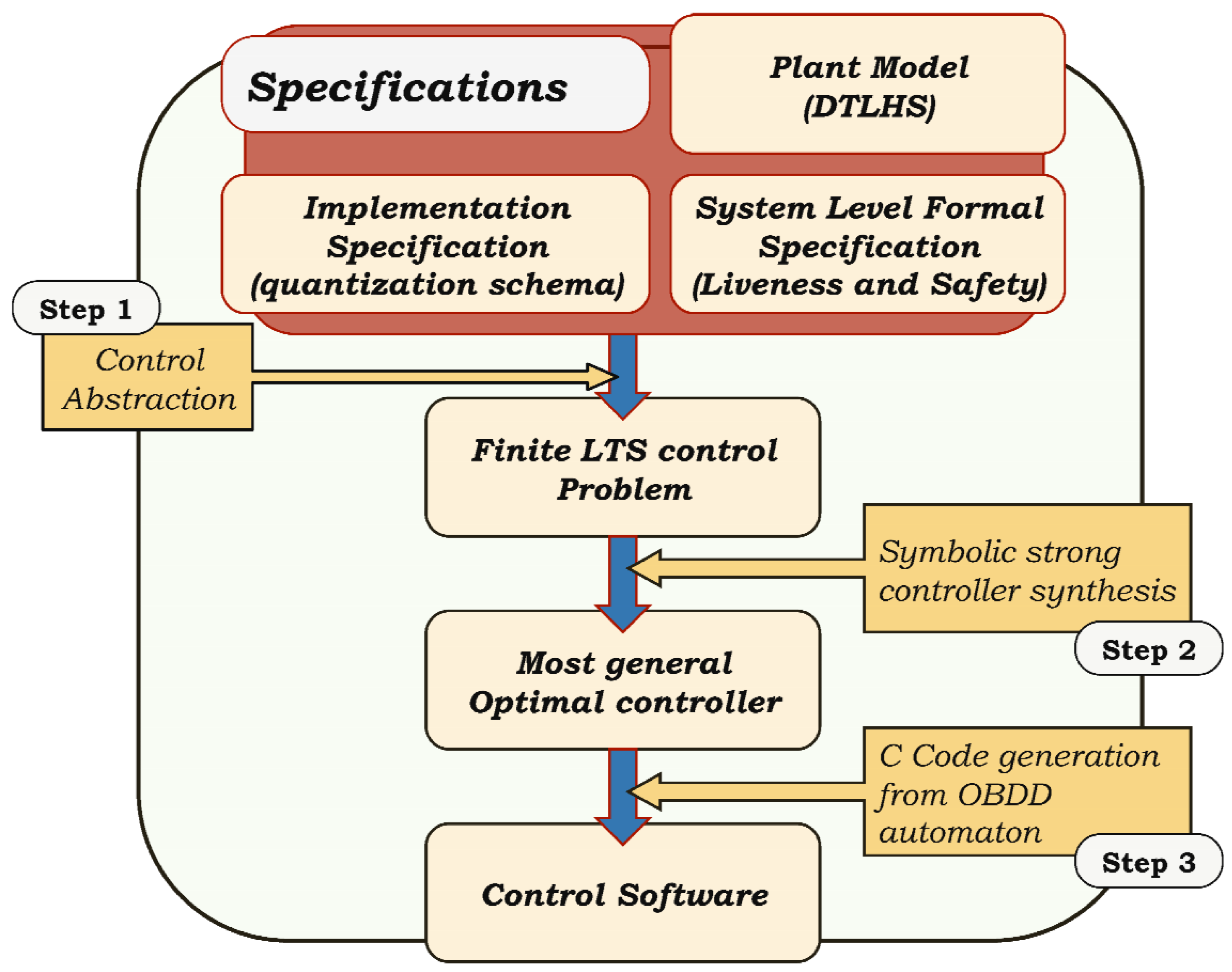
Figure 2 shows the control software synthesis flow that we consider here [10]. We model the controlled system (i.e., the plant) as a DTLHS (Section 2.4), that is a discrete time hybrid system whose dynamics is modeled as a linear predicate (Section 2.1) over a set of continuous as well as discrete variables. The behavior (i.e., semantics) of a DTLHS is given in terms of a Labeled Transition System (LTS, Section 2.3).
Given a plant H modeled as a DTLHS, a set of goal states G (liveness specifications) and an initial region I, both represented as linear predicates, we are interested in finding a restriction K of the behavior of H such that in the closed loop system all paths starting in a state in I lead to G after a finite number of steps. Finding K is the DTLHS control problem (Section 2.4) that is in turn defined as a suitable LTS control problem (Section 2.3).
Finally, we are interested in controllers that take their decisions by looking at quantised states, that is, the values that the control software reads after an AD conversion. This is the quantised DTLHS control problem. Controllers K, which are solution of a quantised DTLHS control problem, are the starting point for the method we describe in this paper.

2.1. Predicates

We denote with X = [ x 1 , , x n ] a finite sequence of variables. Each variable x ranges on a known (bounded or unbounded) interval D x either of the reals or of the integers (discrete variables). We denote with D X the set x X D x . Boolean variables are discrete variables ranging on the set B = {0, 1}. Unless otherwise stated, we suppose real variables to range on R and integer variables to range on Z .
A linear expression over a list of variables X is a linear combination of variables in X with rational coefficients. A linear constraint over X (or simply a constraint) is an expression of the form L ( X ) b , where L ( X ) is a linear expression over X and b is a rational constant. Finally, a conjunctive predicate is a conjunction of constraints.

2.2. OBDD Representation for Boolean Functions

We will denote boolean functions f : B n B with boolean expressions on boolean variables involving + (logical OR), · (logical AND, usually omitted thus x y = x · y ), ¯ (logical complementation) and ⊕ (logical XOR). We will also denote vectors of boolean variables in boldface, e.g., x = x 1 , , x n . Moreover, we also denote with f | x i = g ( x ) the boolean function f ( x 1 , , x i 1 , g ( x ) , x i + 1 , , x n ) . Note that, with such notation, we have that x i . f ( x ) is the boolean function f | x i = 0 ( x ) + f | x i = 1 ( x ) . A truth assignment μ is a partial map from an ordered set of boolean variables V to ( B { } ) | V | . A minterm of μ is a total extension of μ , i.e., a total truth assignment ν : V B | V | s.t. μ ( x ) ν ( x ) = μ ( x ) for all x V . The value of a minterm (or of a total truth assignment) ν is i = 1 n 2 i 1 ν ( x i ) , being V = [ x 1 , , x n ] .
A Complemented edges OBDD (COBDD [44,45]) ρ = ( V , E , r , V , v a r , l o w , h i g h , f l i p , o r d ) is a directed acyclic graph (DAG) ( V , E ) with the following properties:
  • r V is the root of the DAG ρ ;
  • v a r : V V 1 assigns to each vertex v either a variable in V (if v is an internal node) or the unique terminal node 1 (otherwise), so that v a r ( v ) = v a r ( v ) = 1 implies v = v ;
  • the terminal node v s.t. v a r ( v ) = 1 has no children (i.e., the set { v | ( v , v ) E } is empty). In the following, by abusing notation, we will denote with 1 the terminal node itself;
  • each internal node v 1 has exactly two children (i.e., the set S ( v ) = { v | ( v , v ) E } has exactly two elements);
  • h i g h , l o w : V V are partial functions which distinguish the two successors of v as the then-child and the else-child. That is, h i g h ( v ) S ( v ) represents the case in which v a r ( v ) is true (then-child) and l o w ( v ) S ( v ) represents the case in which v a r ( v ) is false (else-child). Both h i g h , l o w are partial since they are not defined on the terminal node 1 ;
  • f l i p : V B is a partial function assigning to each internal node v a boolean value, meaning that the edge ( v , l o w ( v ) ) is complemented. Function f l i p is partial since it is not defined on the terminal node 1 ;
  • on each path from an internal node to the terminal node 1 , the variables labeling each internal node must follow the same ordering o r d . That is, o r d : V { 1 , , | V | } is a bijective function and for all π = v 1 , , v n s.t. ( v i , v i + 1 ) E and v a r ( v n ) = 1 , it must hold that o r d ( v a r ( v i ) ) < o r d ( v a r ( v i + 1 ) ) for all i = 1 , , n 2 .
Given a COBDD ρ , its semantics is a boolean function depending on boolean variables in v a r ( V ) . Such semantics, denoted by · ρ , is recursively defined as follows. The semantics of the terminal node 1 w.r.t. flipping bit b is the boolean constant b ¯ , that is,
1 , b ρ : = b ¯ .
The semantics of internal node v w.r.t. flipping bit b, with v a r ( v ) = x , is the boolean function
v , b ρ : = x high ( v ) , b ρ + x ¯ l o w ( v ) , b flip ( v ) . ρ
Finally, the semantics of ρ is r , f l i p ( r ) ρ . We will write v , b instead of v , b ρ when ρ is understood.
In the following, we will always consider reduced COBDDs, that is, COBDDs with the minimum number of nodes among the ones having as semantics the same boolean function. Computing boolean operations on such reduced COBDDs can be efficiently implemented, as described in [44,45,46].

2.3. Most General Optimal Controllers

A Labeled Transition System (LTS) is a tuple S = ( S , A , T ) where S is a (finite or infinite) set of states, A is a finite set of actions, and T is the (possibly non-deterministic) transition relation of S . A controller for an LTS S is a function K : S × A B enabling actions in a given state. We denote with dom ( K ) the set of states for which a control action is enabled. An LTS control problem is a triple P = ( S , I , G ) , where S is an LTS and I , G S . A controller K for S is a strong solution to P iff it drives each initial state s I in a goal state t G , notwithstanding nondeterminism of S . A strong solution K * to P is optimal iff it minimizes path lengths. An optimal strong solution K * to P is the most general optimal controller (we call such a solution an MGO) iff in each state it enables all actions enabled by other optimal controllers. For more formal definitions of such concepts, see [10]. For efficient algorithms to compute MGOs starting from finite-state (nondeterministic) LTSs see [47].

2.4. Discrete Time Linear Hybrid Systems

In this section, we introduce the class of discrete time Hybrid Systems that we use as plant models, namely Discrete Time Linear Hybrid Systems (DTLHSs for short). For a more complete introduction, see [10].
Definition 1.
A Discrete Time Linear Hybrid System is a tuple H = ( X , U , Y , N ) where: X is a finite sequence of present state variables (we denote with X the sequence of next state variables obtained by decorating with all variables in X); U is a finite sequence of input variables; Y is a finite sequence of auxiliary variables; N ( X , U , Y , X ) is a conjunctive predicate over X U Y X defining the transition relation (next state) of the system. Note that X , U , Y may contain discrete as well as continuous variables.
DTLHSs may be used to represent many interesting real-world plants, such as e.g., the multi-input buck DC-DC converter used in Section 5.
Given a DTLHS H = (X, U, Y, N), we define its behavior (i.e., dynamics) as L T S ( H ) = ( D X , D U , N ˜ ) where: N ˜ : D X × D U × D X B is a function s.t. N ˜ ( x , u , x ) y D Y . N ( x , u , y , x ) . A statex for H is a state x for LTS ( H ) . A DTLHS control problem P = ( H , I , G ) is defined as the LTS control problem ( L T S ( H ) , I, G).
In classical control theory, the concept of quantisation has been introduced (e.g., see [48]) in order to manage real valued variables in (discrete) control software. Quantisation is the process of approximating a continuous interval by a set of integer values. Formally, a quantisation function γ for a real interval I = [ α , β ] is a non-decreasing function γ : I Z s.t. γ ( I ) is a bounded integer interval. In the following, we will only consider uniform quantisations. That is, all quantisation functions γ are defined so that [ α , β ] is divided in 2 b equal intervals, and γ ( x ) = v iff x lays inside the v-th interval, with 0 v 2 b 1 . As a result, γ 1 ( v ) is an interval for all 0 v 2 b 1 . In the following, we will define a uniform quantisation function γ by only providing b as the number of bits. We will also refer to the quantisation function step of γ , notation γ , as | I | 2 b .
Finally, a quantisation Q = ( A , Γ ) for a DTLHS encloses the set of quantisation functions Γ , containing a quantisation function γ x (as discussed above, γ x N is the number of bits to be used in the quantisation) for all state and action variables x X and u U (in the following, we will refer to Γ 1 with the set of all γ x 1 ), as well as the bounded (safe) admissible regionA on which the desired controller is supposed to work. Namely, A bounds both state variables (subregion A X ) on which the controller has to keep the system and action variables (subregion A U ) on which the controller works. The quantisation step Γ is defined as m a x { γ | γ Γ } . Again, given all admissible regions A, a quantisation can be defined by only providing the number of bits b x for each variable x X .
By applying a quantisation to the dynamics LTS ( H ) of a DTLHS H we obtain a finite-state LTS. A control problem admits a quantised solution if control decisions can be made by just looking at quantised values (i.e., considering only the finite-state LTS). This enables a software implementation for a controller, as well as usage of algorithms mentioned in Section 2.3 in order to compute controllers. To accommodate quantisation errors, always present in software based controllers, it is useful to relax the notion of control solution by tolerating the error on the continuous variables to be at most the quantisation step. Accordingly, we look for controllers that drive the plant to the goal G with an error at most Γ (we call such a controller a Γ -solution to P ). Definition 2 formalizes the above concepts.
Definition 2.
Given a quantisation Q , a Q Quantised Feedback Control (QFC) solution to a DTLHS control problem P is a Γ solution K ( x , u ) to P such that K ( x , u ) = K ^ ( Γ ( x ) , Γ ( u ) ) , where K ^ : Γ ( A X ) × Γ ( A U ) B .
For efficient (non-complete) algorithms to compute QFC solutions to a DTLHS control problem, for example, see [10]. The approach we present here (Section 4) takes as input a controller which is a QFC solution of a DTLHS control problem.

Controllers and COBDDs

By Definition 2, K is based on a controller K ^ that only looks at integer (quantised) values. Thus, by considering the boolean encoding of such values (as it is usual in Model Checking applications), we have that K ^ , and by abuse of notation K, can be represented as a COBDD ρ s.t. ρ = K . More formally, given Q = ( A , Γ ) , for all x X , we need a set of Γ x boolean variables e n c ( x ) = [ x 1 , , x Γ x ] in order to encode x (and analogously for actions u U ). This implies that, in the resulting COBDD ρ , the set of boolean variables V (which is the target set for labeling function v a r ) consists of the boolean variables x = [ e n c ( x 1 ) , , e n c ( x | X | ) ] for the state and u = [ e n c ( u 1 ) , , e n c ( u | U | ) ] for the action.

3. Other Related Work

This article is an extended and completely revised version of [49]. With respect to [49], this paper provides more details in all article sections, including revised and enriched experiments.
Many papers (e.g., see [10,11,50,51,52,53,54]) tackling the problem of synthesizing control software (which looks tato quantized states) or control laws (which look at real states) of hybrid systems show pictures of the type we generate in this paper (with r = 1 , i.e., only one bit for the actions). However, to the best of our knowledge there are no papers directly focusing on the method to generate such pictures, thus no automatic approach to controllers visualization is described.
An entire area of Computer Science is dedicated to Visualization, that is, to using (often parallel) algorithms to visualize scientific data (see [55] for a survey). Such algorithms are tailored to visualize data coming from given application domains, such as Biology (see, e.g., [56,57]), Medicine (see, e.g., [58,59,60,61]), Mathematics (see, e.g., [62]), and more specifically, for example, in weather forecasting (see, e.g., [63]), in cellular screen visual analysis (see, e.g., [64]) and in taxi trajectories [65]. Such works typically start from a huge amount of available data to be visualized, whilst here our starting point is an OBDD representing a controller. Moreover, we focus on a field, that is, visualization of control software, which is not considered by works in the topics of Visualization. Finally, the OBDD-based method described here to obtain the final pictures is not used in Visualization.
Therefore, to the best of our knowledge this is the first time that an algorithm generating a picture of the coverage of a controller for a DTLHS is presented.

4. Automatic Visualization of Control Software

In this section, we describe (Algorithms 1 and 2) our method to automatically generate a 2D picture giving a human-readable representation of a Q QFC solution K to a DTLHS control problem P = ( H , I , G ) with a given quantisation Q = ( A , Γ ) .
The picture we generate lies on a 2D Cartesian plane. If H has exactly 2 state variables, then each axis of the picture is labeled with a state variable of H and has a range bounded by A. The key property is the following: a point ( x , y ) in the picture is colored depending on which action set is enabled by K in the DTLHS state ( x , y ) , that is, on
c ( x , y ) = { u | K ( ( x , y ) , u ) = 1 } .
If H has l + 2 state variables with l > 0 (i.e., if | X | = l + 2 ), then our method requires us to choose which variables have to be used as axis labels. That is, as a further input a partition of X in two sets { x , y } and { d 1 , , d l } is needed. Given this, the action set we consider for each point ( x , y ) in the Cartesian space is c ( x , y ) = { u | d 1 , , d l . K ( ( x , y , d 1 , , d l ) , u ) = 1 } . This entails that in the output picture a state ( x , y ) is colored iff there exists at least a value for all plant state variables { d 1 , , d l } that is controlled by K.
Note that the picture output by our approach is practically useful if H has at least two real variables, which is indeed the case in most real-world SBCSs. Finally, a second picture showing the correspondence between action sets and colors is also generated, so that the first one may be easily interpreted.
Algorithm 1 Visualizing a controller.
Require: 
DTLHS H , quantisation Q = ( a , Γ ) , state variables set Ξ s.t. | Ξ | = 2 , COBDD ρ = ( V , E , r , V , v a r , l o w , h i g h , f l i p , o r d )
Ensure: 
Visualize( H , Q , Ξ , ρ ):
 1:
let n = x Ξ Γ x and a = u U Γ u
 2:
let e n c be the encoding defined by Q on X and U
 3:
let x X \ Ξ e n c ( x ) = { v 1 , , v }
 4:
let v , b be s.t. v , b ρ = v 1 , , v . ρ
 5:
let ρ = ( V , E , r , V , v a r , l o w , h i g h , f l i p , o r d ) be s.t. i) ρ ρ = ρ ρ and ii) o r d ( w ) = o r d ( w ) a if o r d ( w ) > a , and o r d ( w ) = o r d ( w ) + n otherwise
 6:
M CreateGnuplotBody( ρ , f l i p ( r ) , n , , )
 7:
M CompactSameColorRegions(M)
 8:
χ LexOrderedDiffColorsRGB( { ( v , b ) | μ s.t. ( μ , v , b ) M } )
 9:
P , C ,
 10:
for all triples ( μ , v , b ) M do
 11:
 using Q , append to P the rectangle corresponding to μ with color χ ( ( v , b ) )
 12:
for all ( v , b ) s.t. ( μ , v , b ) M do
 13:
 append to C a rectangle of color χ ( ( v , b ) ) with label S a t A l l ( ρ , v , b )
 14:
return P , C
Algorithm 2 Visualizing a controller: Gnuplot body.
Require: 
COBDD ρ = ( V , E , r , V , v a r , l o w , h i g h , f l i p , o r d ) , flipping bit b, number of state boolean variables n, truth assignment μ , (assignment, COBDD node, flipping bit) triples set M
Ensure: 
CreateGnuplotBody( ρ , b , a , μ , M ):
 1:
c b
 2:
if ( v = 1 ¬ c ) ∨ ( v 1 o r d ( v a r ( v ) ) > n ) then
 3:
 for all minterms ν of μ do
 4:
   M M ( ν , v , c )
 5:
else if v 1 then
 6:
μ ( v a r ( v ) ) 1
 7:
M CreateGnuplotBody( ρ , h i g h ( v ) , c , n , μ , M )
 8:
μ ( v a r ( v ) ) 0
 9:
 if f l i p ( v ) then c ¬ c
 10:
M CreateGnuplotBody( ρ , l o w ( v ) , c , n , μ , M )
 11:
returnM

4.1. Input and Output

In order to generate the two pictures with the properties described above, we design a function Visualize (described in Algorithm 1), which takes as input:
  • A DTLHS plant model H = ( X , U , Y , N ) ;
  • A quantisation Q = ( A , Γ ) for H . Such quantisation specifies (i) how many bits are used to discretize variables in X and in U and (ii) the bounds of variables in X and U;
  • A subset Ξ X of plant state variables s.t. | Ξ | = 2 . Variables in Ξ are those to be shown in the axes of the final 2D picture. If | X | = 2 , then Ξ = X ;
  • A Q QFC solution K to a control problem involving H , represented as a COBDD ρ s.t. ρ = K .
The output of Visualize is a Gnuplot [12] source files pair ( P , C ) describing the picture P to be generated and the color legend C. Note, however, that Visualize may be easily adjusted to work with any other graphing tool, provided that it generates pictures from textual descriptions. In Algorithm 1, we represent P as a list of rectangles in the plant state space (restricted to variables in Ξ ). To each rectangle, we associate the RGB code of the corresponding color to be displayed. Analogously, C is a list of colored rectangles with height equal to the height of the picture: on the x axis the action set corresponding to each colored rectangle is shown. If too many action sets are used in P, then C may be split in many pictures in order to retain readability.

4.2. Algorithm Details

Function Visualize works as follows. First of all, in line 1 the number of boolean variables needed to encode the plant state variables in Ξ and action variables in U are computed as n and a respectively. Then, in lines 2–4, state boolean variables encoding plant state variables not in Ξ (i.e., those not to be displayed in the final picture) are existentialised out from K, thus obtaining COBDD node v and flipping bit b such that v , b = v 1 , , v . ρ = v 1 , , v . K = K ˜ . As a result, the final picture will show all values for plant state variables in Ξ s.t. there exists at least a value for all plant state variables in X \ Ξ that is controlled by K.
In order to generate the desired picture, we need to visit the COBDD ρ starting from the node v with the flipping bit b computed above, so as to obtain an action set. That is, we want to traverse ρ starting from v so as to arrive to a node v ˜ s.t. the COBDD rooted in v ˜ is only labeled with action boolean variables. In formulas, we want to find all v ˜ , b ˜ s.t. v ˜ , b ˜ ρ = F ( u ) , i.e., F does not depend on state variables in x, but only on action variables in u. In order to do this, we need state variables to come before action variables in the ordering defined by function o r d , i.e., o r d ( v x ) < o r d ( v u ) for all v x e n c ( x ) , v u e n c ( u ) s.t. x X , u U . However, in order to obtain a better compression, controllers are represented with COBDDs where the ordering function o r d is s.t. o r d ( v x ) > o r d ( v u ) [10]. Hence, by using standard COBDD reordering algorithms [44,45], line 5 changes the ordering to be the desired one, thus obtaining a new COBDD ρ representing the same function of ρ , that is, K ˜ .
This allows us to perform a depth-first search (DFS in the following) of the COBDD ρ representing K ˜ , by calling (line 6) function CreateGnuplotBody described in Algorithm 2. The goal of function CreateGnuplotBody (see Section 4.2.1) is to return a list M of ( μ , w, c) triples s.t. μ is a total truth assignment to all state boolean variables, w is a node of COBDD ρ and c is a flipping bit. For each triple ( μ , w, c) in M, the following holds: if x ^ is the value of μ (i.e., x ^ is a quantised state described by the variables in Ξ ), then w , c is the (boolean) characteristic function of the action set enabled by K ˜ in x ^ . That is, w , c = F s.t. F ( u ^ ) holds iff K ˜ ( x ^ , u ^ ) holds. Note that, by definition of K ˜ , this entails that for all plant states x in the quantised state x ^ (i.e., such that x Γ 1 ( x ^ ) ) K enables the set of actions u s.t. the boolean encoding of u (i.e., u ^ ) satisfies w , c .
Once function CreateGnuplotBody has finished, the returned list M may be directly translated in a Gnuplot file P as follows. For each triple ( μ , w , c ) in M, the value x ^ of μ is translated in a rectangle having as bounds those of Γ 1 ( x ^ ) , that is, of the Cartesian product of the intervals that are mapped to x ^ (line 11). The RGB color of such a rectangle may be determined starting from the address (a C language pointer) of w, also taking into account the flipping bit c. However, this has the following drawbacks: (i) the Gnuplot file for the picture may be too big; (ii) different runs of function Visualize (e.g., with different quantisations, and thus different boolean encoding, for plant state variables) may result in different colors for equal action sets, which may make difficult an effective comparison between different experiments. In order to counteract (i), M is compacted, by collapsing contiguous quantised states with the same action sets (function CompactSameColorRegions in line 7 of Algorithm 1). This is performed by a greedy sub-optimal procedure, which first compacts vertically all adjacent rectangles with the same color and then compacts the resulting rectangles horizontally. In order to avoid (ii), we first generate all the needed colors, that is, those corresponding to action set in A = { ( w , c ) | μ s.t. ( μ , w , c ) M } (line 8). Then, we use a lexicographical ordering on A to pick one of such colors. This is done by actually considering all actions enabled by w , c , so that we always obtain the same colors associated to the same action sets.
Note that generating many distinguishable colors is by itself a non-trivial problem [66,67]. In this work, we rest on a technique which generates equally spaced colors in the H-dimension of the HSV (Hue Saturation Value) color space [68], and then converts them back into the RGB space using fixed values for S and V (in our experiments, we fix V = 0.95 and S = 0.5) and standard algorithms [69]. Namely, we start from c 1 = 0.5 and then, for all color pairs ( c i , c i + 1 ) s.t. c i + 1 is generated immediately after c i , we have that H ( c i + 1 ) = f r a c ( H ( c i ) + Φ ) , being H the H-dimension in the HSV color space, Φ = 5 1 2 0.618033988749895 the golden ration conjugate and f r a c ( x ) = x x the fractional part of x. Using more complex (and more expensive from a computational point of view) techniques, like e.g., [66], may improve pictures readability.
Finally, the Gnuplot file C maintaining the correspondence between colors and action sets is generated in lines 12–13, where SatAll returns all satisfying minterms of the boolean function represented by the given COBDD. If this results in too many colors, C is split in many files in order to retain readability.
We remark that, by using the above described technique for generating distinguishable colors, we are not giving a special meaning to the colors we are using. That is, our approach would equally work if, e.g., we swap the colors assigned to two different action sets. As a result, we would obtain a differently colored figure P, and a different figure C giving the new legend. Summing up, using colors is, in our approach, a means to visualize which action set is used in a given state region, by simultaneously considering the two figures P (where colors are used) and C (where colors meaning, in terms of action set, are provided).

4.2.1. Function CreateGnuplotBody

Function CreateGnuplotBody (Algorithm 2) essentially performs a DFS of COBDD ρ starting from the root r with flipping bit f l i p ( r ) . We recall that, when CreateGnuplotBody is called at line 6 of Algorithm 1, the COBDD ρ resulting from having changed the variables ordering and having existintialised on “non-interesting” variables is passed. On each path from r to 1 , such DFS stops as soon as an action boolean variable is found at node v and flipping bit c. In fact, if o r d ( v a r ( v ) ) > n (line 2), then we have passed the mark for plant state boolean variables, and hence the sub-tree rooted in v will only contain nodes labeled with action boolean variables (as a consequence of variable reordering discussed above). While exploring such a path, the corresponding (partial) truth assignment μ is maintained, that is, if the then edge of a node w has been traversed, then μ ( v a r ( w ) ) is set to 1 (lines 6–7); if the else edge has been traversed, then μ ( v a r ( w ) ) is set to 0 (lines 8–10). Moreover, if a complemented edge is traversed, the flipping bit b is flipped (line 9). Once the current path ends in a node v labeled by an action boolean variable (line 2), the to-be-returned list M is updated (lines 3–4) by adding all minterms of the current μ together with the action set ( v , c ) . Line 2 also detects the case in which 1 is reached without passing through action variables. In this case, if the flipping bit is 0 (i.e., no complementation required) then all actions are enabled by K for the quantised states corresponding to values of minterms of μ , thus all minterms of μ are added to M. Otherwise, if the flipping bit is 1, then no action is enabled for the quantised states corresponding to values of minterms of μ (i.e., the corresponding action set is ), thus no minterms are added.

5. Experimental Results

We implemented our picture generation algorithm in the C programming language, using the CUDD (Colorado University Decision Diagram) package for OBDD based computations and BLIF (Berkeley Logic Interchange Format) files to represent input OBDDs. We name the resulting tool KPS (Kontroller Picture Synthesizer). KPS is part of a more general tool named QKS (Quantized feedback Kontrol Synthesizer [10]). In this section we present our experiments that aim at evaluating effectiveness of KPS.

5.1. Experimental Settings: Case Study

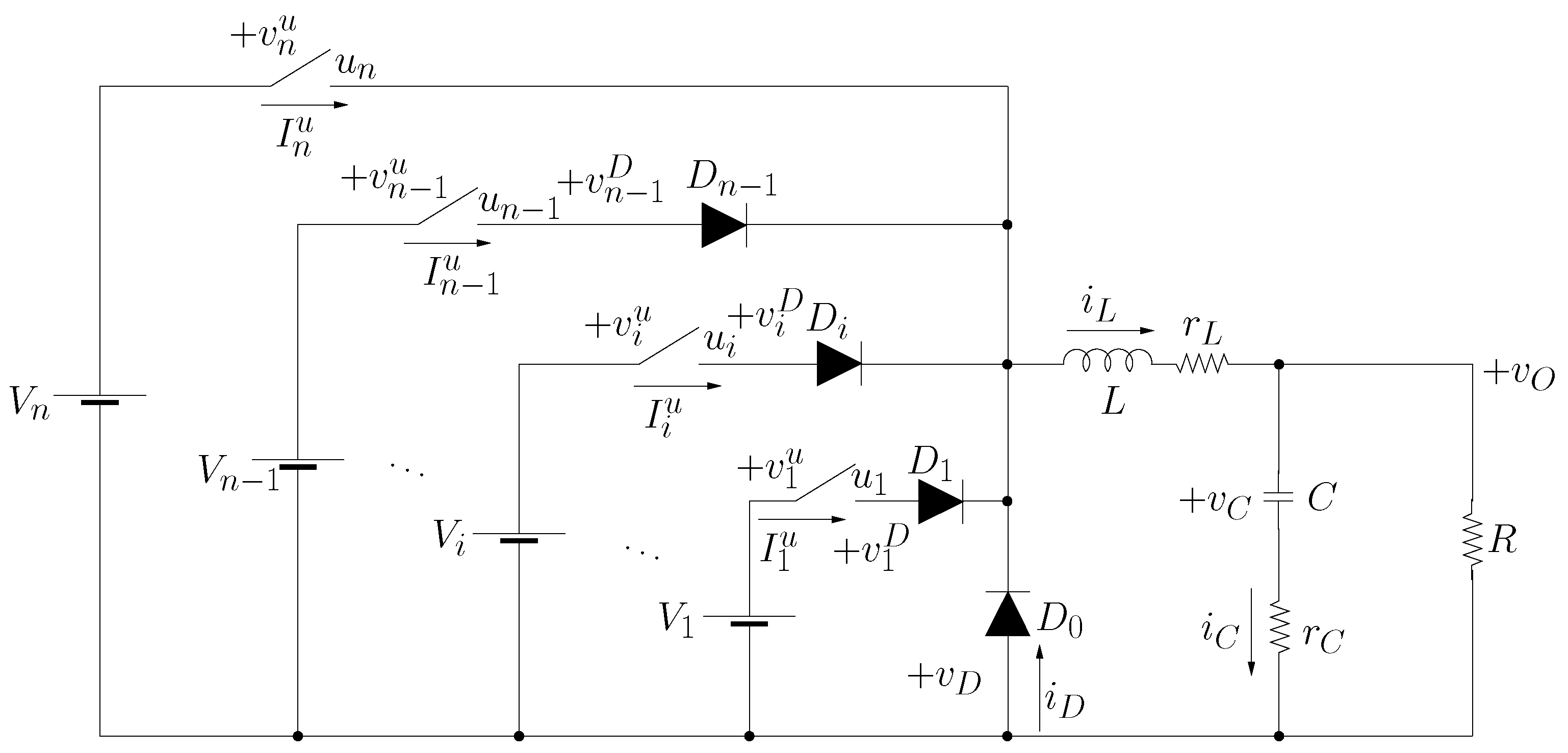
The experimental results in this paper refer to the multi-input buck DC-DC converter [70] (Figure 3) case study. Namely, a multi-input buck DC-DC converter is a cyber-physical control system where the plant is a mixed-mode analog circuit converting the DC input voltage ( V i in Figure 3) to a desired DC output voltage ( v O in Figure 3), and the controller computes actions to actuate some circuit switches in order to maintain current and voltage within given bounds. As an example, buck DC-DC converters are used off-chip to scale down the typical laptop battery voltage (12–24) to the just few volts needed by the laptop processor (e.g., [71]) as well as on-chip to support Dynamic Voltage and Frequency Scaling (DVFS) in multicore processors (e.g., [72]). Because of its widespread use, control schemas for buck DC-DC converters have been widely studied (e.g., see [71,72]). The typical software based approach (e.g., see [71]) is to control the switches u 1 , , u n in Figure 3 (typically implemented with a MOSFET) with a microcontroller.
In such a converter (Figure 3), there are n power supplies with voltage values V 1 , , V n , n switches with voltage values v 1 u , , v n u and current values I 1 u , , I n u , and n input diodes D 0 , , D n 1 with voltage values v 0 D , , v n 1 D and current i 0 D , , i n 1 D .
The typical goal for a multi-input buck is to drive i L and v O within given goal intervals. In our case study, we have that the goal is defined by the linear constraints 2 i L 2 and 4.99 v O 5.01 .

5.2. Experimental Settings: Running KPS

For our experiments, we consider four controllers for buck DC-DC converters with i inputs, being i { 1 , 2 , 3 , 4 } , generated by QKS as described in [11]. We denote the DTLHS representing the buck with i inputs as H i , and with ρ i the COBDD representing the controller K i ( x , u ) for H i as generated by QKS. Quantizations for such DTLHSs is Q is s.t. n = | x | = 20 and a i = | u | = i . For each ρ i , we run KPS so as to compute Visualize( H i , Q , X , ρ i , v i , b i ) (see Algorithm 1). All our experiments have been carried out on a 3.0 GHz Intel hyperthreaded Quad Core Linux PC with 8 GB of RAM.

5.3. KPS Performance

In this section we will show the performance (in terms of computation time and output size) of the algorithms discussed in Section 4. Table 1 shows our experimental results. The i-th row in Table 1 corresponds to experiments running KPS so as to compute Visualize( H i , Q , X, ρ i , v i , b i ) (see Algorithm 1). Columns in Table 1 have the following meaning. Column a shows the number of action variables | u | (note that | x | = 20 on all our experiments). Column CPU(P) shows the computation time of KPS, that is, of function Visualize of Algorithm 1 (in seconds). Columns | P | , | J | and | E | show the size in KB of, respectively, the source Gnuplot file for the 2D picture (i.e., the output P of function Visualize of Algorithm 1), the JPEG (Joint Photographic Experts Group) file generated by Gnuplot from P (i.e., with compression), and the EPS (Encapsulated Postscript) file generated by Gnuplot from P (i.e., without compression). Finally, Column CPU(G) shows the computation time of Gnuplot (in seconds) to generate the JPEG and the EPS files (computation time and size for file C are negligible).
From Table 1 we can see that, in slightly more than 10 s we are able to generate the Gnuplot file for the multi-input buck with a = 4 action variables. Then, Gnuplot needs about one hour to synthesize the actual picture (either in JPEG or in EPS).

5.4. Controllers Qualitative Evaluation via Pictures

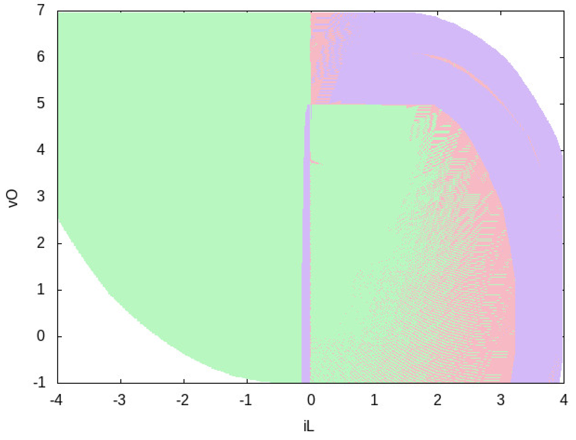
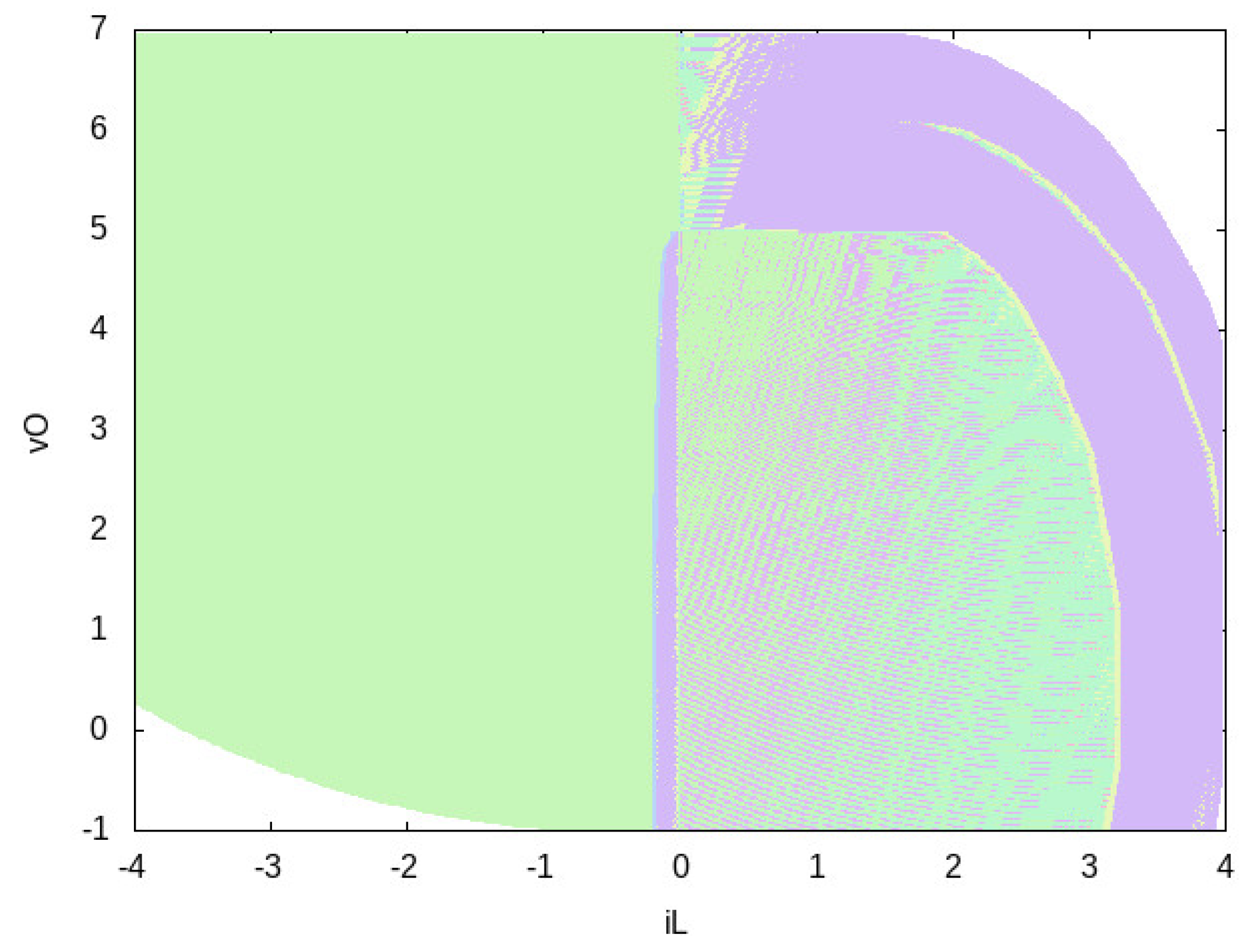
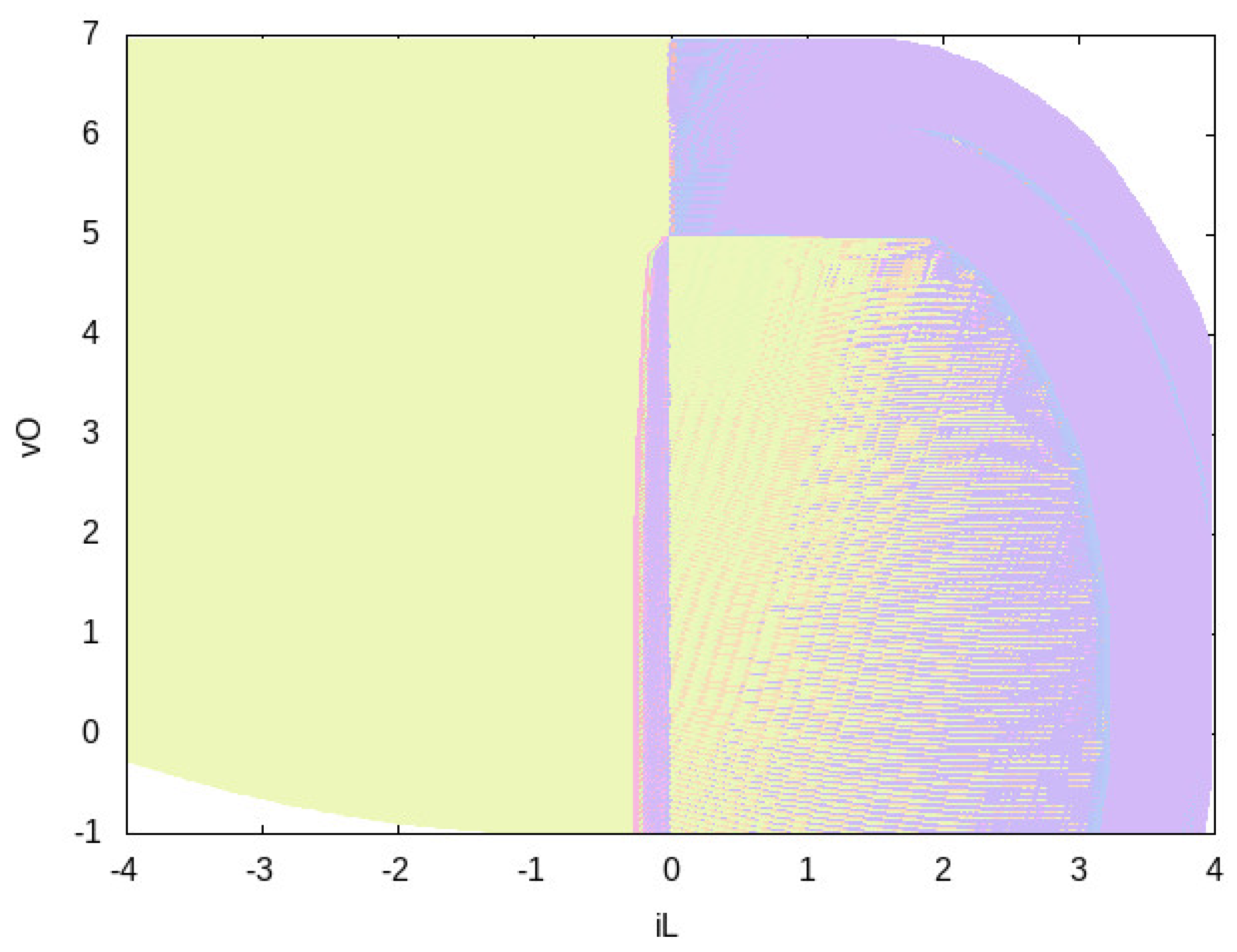
In Figures 4, 6, 8 and 9 we show the output P generated by the KPS–Gnuplot chain for K 1 , , K 4 . Moreover, in Figures 5 and 7 we show the output C (i.e., colors legend) generated by the KPS–Gnuplot chain for K 1 and K 2 .
We now show how we may answer to the questions exemplified in Section 1 (plus one), thanks to Figure 4, Figure 5, Figure 6, Figure 7, Figure 8 and Figure 9:
  • Do K 1 , , K 4 cover a wide enough portion of the system state space? The answer is yes for all controllers K 1 , , K 4 , since the region for which any color is shown covers nearly all the system state space. Moreover, we may see that, increasing the number of actions (i.e., going from K 1 to K 4 ) the coverage increases.
  • Do K 1 , , K 4 cover the most important portion of the system state space? Again, the answer is yes for all controllers K 1 , , K 4 . Namely, in the DC-DC buck converter case study the most important part is the starting point i L = 0 , v O = 0 and the goal region (delimited by 2 i L 2 A and 4.99 v O 5.01 V). In all four cases, it is clear that such regions are covered.
  • Which actions are enabled by K 1 , , K 4 in a given portion of the system space? If we focus on the whole covered state space, we have the following. From Figure 5 we may immediately see that all possible actions sets are used by K 1 . On the other hand, from Figure 7 we immediately conclude that only 7 actions sets out of 2 2 2 1 = 15 (excluding the empty actions set) are indeed enabled in K 2 . Note that, in order to retain readability, colors legend pictures always have at most 3 colors. If more than n > 3 actions sets are used by the given controller, then n 3 pictures for colors legend are used. This results in 1 picture for K 1 and in 3 pictures for K 2 . For space reasons, we do not show colors legends for K 3 and K 4 . Namely, K 3 uses 25 actions set (out of 255), resulting in 9 files for colors legend, whilst K 4 uses 83 actions sets (out of 65,535), resulting in 28 files for colors legend.
  • Is there an actions set which is used more than the other actions sets? We have that the most used actions sets are { 1 } for K 1 and { ( 0 , 1 ) , ( 1 , 1 ) } for K 2 . By considering the missing colors legend pictures, analogous results may be obtained for K 3 and K 4 .
  • Which is the distribution of action sets on the state space? Let us focus, e.g., on Figure 4. We have a huge portion on the left part of the picture which is colored in green, which corresponds to action u1 = 1 (see Figure 5). This may be interepreted as follows: for negative values of i L (provided that v O is not too small w.r.t. i L ), the only action enabled by the controller is always to close the switch u 1 (see Figure 3). As a further example, if 2 i L 3 A and v O < 2 V, then there are some states for which u1 = 1 (switch closed, green color in Figure 5) and some other for which it is ok to perform any action (either close or open the switch is ok, pink color in Figure 5).

6. Conclusions and Future Work

In this paper, we addressed the problem of providing a graphical human-readable representation (i.e., of visualizing) a controller K for a software-based control system, represented as a discrete-time linear hybrid system (DTLHS). Such a representation is useful for allowing a human designer to have a qualitative measure of the controller behavior. To this aim, we presented an algorithm and a tool KPS implementing it, which, from an OBDD representation of K, effectively generates a 2D picture depicting K. Such a picture consists of a Cartesian plane where each point corresponds to a state of the starting DTLHS, and assigns the same color to all regions of states for which the same actions set is defined on K. A separated set of pictures showing the relation between a color and the corresponding actions set is also automatically generated. In this way, the state region for which any color is shown depicts the coverage of K, whilst the regions colors give a glimpse of which actions are turned on by K on given plant states regions. We have shown feasibility of our proposed approach by presenting experimental results on using it to visualize the controller for a multi-input buck DC-DC converter. Such experimental results show that our automatically generated pictures may indeed answer important qualitative questions above the controller behavior.
The proposed approach currently generates a 2D picture, which works well for systems with two plant state variables. A useful extension of the proposed approach would be to synthesise an interactive 3D picture in essentially the same way as we do here, by generating parallelepipeds instead of rectangles. Such an approach would work well for systems with at least three state variables. Having an interactive picture would allow the designer to rotate or zoom the picture, so as to explore hidden regions.
An interesting future research direction is also to investigate a different graphical representation of a given controller, in order to work well with any number of state variables. As an example, a 3D bar picture may be generated so that for each quantized value of the two variables to be shown (i.e., those in Ξ in the notation of Section 4.1) a bar shows the percentage of coverage w.r.t. variables not to be shown (i.e., not in Ξ ). Moreover, we plan to show how we can use our approach to qualitatively compare different controllers for the same plant, obtained by changing some key parameters in the plant model. Furthermore, we plan to apply our approach to other areas in which OBDDs or OBDD-like data structures are used, such as symbolic formal verification, system-level formal verification and statistical model checking.

Author Contributions

All authors have equally contributed to the present paper. All authors have read and agreed to the published version of the manuscript.

Funding

This work was partially supported by the following research projects/grants: Italian Ministry of University & Research (MIUR) grant “Dipartimenti di Eccellenza 2018–2022” (Dept. Computer Science, Sapienza Univ. of Rome); EC FP7 project SmartHG (Energy Demand Aware Open Services for Smart Grid Intelligent Automation, 317,761); INdAM “GNCS Project 2018”.

Institutional Review Board Statement

Not applicable.

Informed Consent Statement

Not applicable.

Data Availability Statement

All data used for this paper have been described within the paper itself.

Conflicts of Interest

The funders had no role in the design of the study; in the collection, analyses, or interpretation of data; in the writing of the manuscript, or in the decision to publish the results.

Abbreviations

The following abbreviations are used in this manuscript:
ADAnalog-to-Digital
BLIFBerkeley Logic Interchange Format
COBDDComplemented edges OBDD
CUDDColorado University Decision Diagram
DADigital-to-Analog
DAGDirected Acyclic Graph
DFSDepth-First Search
DTLHSDiscrete Time Linear Hybrid System
EPSEncapsulated Postscript
FDRIFault Detection, Isolation and Recovery
HSVHue Saturation Value
JPEGJoint Photographic Experts Group
KPSKontroller Picture Synthesizer
LTSLabeled Transition System
MGOMost General Optimal controller
MILPMixed Integer Linear Programming
OBDDOrdered Binary Decision Diagram
QFCQuantized Feedback Control
QKSQuantized feedback Kontrol Synthesizer
RGBRed Green Blue
SBCSSoftware Based Control Systems

References

  1. Lee, E.A.; Seshia, S.A. Introduction to Embedded Systems, A Cyber-Physical Systems Approach; MIT Press: Cambridge, MA, USA, 2017. [Google Scholar]
  2. Bartocci, E.; Deshmukh, J.; Donzé, A.; Fainekos, G.; Maler, O.; Ničković, D.; Sankaranarayanan, S. Specification-based monitoring of cyber-physical systems: A survey on theory, tools and applications. In Lecture Notes in Computer Science (including Subseries Lecture Notes in Artificial Intelligence and Lecture Notes in Bioinformatics); Springer: Berlin/Heidelberg, Germany, 2018; pp. 135–175. [Google Scholar] [CrossRef]
  3. Gawand, H.L.; Bhattacharjee, A.; Roy, K. Online Monitoring of a Cyber Physical System Against Control Aware Cyber Attacks. Procedia Comput. Sci. 2015, 70, 238–244. [Google Scholar] [CrossRef] [Green Version]
  4. Henzinger, T.A.; Sifakis, J. The Embedded Systems Design Challenge. In Proceedings of the International Symposium on Formal Methods, Hamilton, ON, Canada, 21–27 August 2006; pp. 1–15. [Google Scholar]
  5. Henzinger, T.; Ho, P.H.; Wong-Toi, H. HyTech: A Model Checker for Hybrid Systems. STTT 1997, 1, 110–122. [Google Scholar] [CrossRef]
  6. Frehse, G. PHAVer: Algorithmic verification of hybrid systems past HyTech. Int. J. Softw. Tools Technol. Transf. 2008, 10, 263–279. [Google Scholar] [CrossRef]
  7. Wong-Toi, H. The synthesis of controllers for linear hybrid automata. In Proceedings of the CDC, San Diego, CA, USA, 10–12 December 1997; Volume 5, pp. 4607–4612. [Google Scholar] [CrossRef]
  8. Tomlin, C.; Lygeros, J.; Sastry, S. Computing Controllers for Nonlinear Hybrid Systems. In Proceedings of the HSCC, Berg en Dal, The Netherlands, 29–31 March 1999; pp. 238–255. [Google Scholar]
  9. Mazo, M.; Davitian, A.; Tabuada, P. PESSOA: A Tool for Embedded Controller Synthesis. In International Conference on Computer Aided Verification (CAV), Proceedings of the 22nd International Conference, CAV 2010, Edinburgh, UK, 15–19 July 2010; Springer: Berlin/Heidelberg, Germany, 2010; pp. 566–569. [Google Scholar]
  10. Mari, F.; Melatti, I.; Salvo, I.; Tronci, E. Model Based Synthesis of Control Software from System Level Formal Specifications. ACM TOSEM 2014, 23, 1–42. [Google Scholar] [CrossRef]
  11. Alimguzhin, V.; Mari, F.; Melatti, I.; Salvo, I.; Tronci, E. A Map-Reduce Parallel Approach to Automatic Synthesis of Control Software. In Proceedings of the International SPIN Symposium on Model Checking of Software (SPIN 2013), Stony Brook, NY, USA, 8–9 July 2013; Springer: Berlin/Heidelberg, Germany, 2013; Volume 7976, pp. 43–60. [Google Scholar] [CrossRef] [Green Version]
  12. Janert, P.K. Gnuplot in Action: Understanding Data with Graphs; Manning Publications Co.: Greenwich, CT, USA, 2009. [Google Scholar]
  13. Clarke, E.M.; Grumberg, O.; Peled, D.A. Model Checking; The MIT Press: Cambridge, MA, USA, 1999. [Google Scholar]
  14. Sirjani, M.; Lee, E.A.; Khamespanah, E. Verification of Cyberphysical Systems. Mathematics 2020, 8, 1068. [Google Scholar] [CrossRef]
  15. Sirjani, M.; Lee, E.A.; Khamespanah, E. Model Checking Software in Cyberphysical Systems. In Proceedings of the 2020 IEEE 44th Annual Computers, Software, and Applications Conference (COMPSAC), Madrid, Spain, 13–17 July 2020; pp. 1017–1026. [Google Scholar] [CrossRef]
  16. Burch, J.R.; Clarke, E.M.; McMillan, K.L.; Dill, D.L.; Hwang, L.J. Symbolic model checking: 1020 states and beyond. Inf. Comput. 1992, 98, 142–170. [Google Scholar] [CrossRef] [Green Version]
  17. Cimatti, A.; Corvino, R.; Lazzaro, A.; Narasamdya, I.; Rizzo, T.; Roveri, M.; Sanseviero, A.; Tchaltsev, A. Formal Verification and Validation of ERTMS Industrial Railway Train Spacing System. In International Conference on Computer Aided Verification (CAV), Proceedings of the 24th International Conference, CAV 2012, Berkeley, CA, USA, 7–13 July 2012; Springer: Berlin/Heidelberg, Germany, 2012; pp. 378–393. [Google Scholar]
  18. Holzmann, G.; Puri, A. A Minimized Automaton Representation of Reachable States. Int. J. Softw. Tools Technol. Transf. (STTT) 1999, 2, 270–278. [Google Scholar] [CrossRef] [Green Version]
  19. Zuliani, P.; Platzer, A.; Clarke, E. Bayesian Statistical Model Checking with Application to Stateflow/Simulink Verification; Formal Methods in System Design; Springer: Berlin/Heidelberg, Germany, 2010; Volume 43, pp. 243–252. [Google Scholar] [CrossRef]
  20. Mancini, T.; Mari, F.; Massini, A.; Melatti, I.; Merli, F.; Tronci, E. System Level Formal Verification via Model Checking Driven Simulation. In Proceedings of the CAV 2013, Saint Petersburg, Russia, 13–19 July 2013; Springer: Berlin/Heidelberg, Germany, 2013; Volume 8044, pp. 296–312. [Google Scholar] [CrossRef]
  21. Mancini, T.; Mari, F.; Massini, A.; Melatti, I.; Tronci, E. System Level Formal Verification via Distributed Multi-Core Hardware in the Loop Simulation. In Proceedings of the PDP 2014, Torino, Italy, 12–14 February 2014; pp. 734–742. [Google Scholar] [CrossRef]
  22. Mancini, T.; Mari, F.; Massini, A.; Melatti, I.; Tronci, E. Anytime System Level Verification via Random Exhaustive Hardware In The Loop Simulation. In Proceedings of the DSD 2014, Verona, Italy, 27–29 August 2014; pp. 236–245. [Google Scholar]
  23. Camilli, M. Formal Verification Problems in a Big Data World: Towards a Mighty Synergy. In Companion Proceedings of the 36th International Conference on Software Engineering; ICSE Companion 2014; Association for Computing Machinery: New York, NY, USA, 2014; pp. 638–641. [Google Scholar] [CrossRef] [Green Version]
  24. Mancini, T.; Mari, F.; Massini, A.; Melatti, I.; Tronci, E. SyLVaaS: System Level Formal Verification as a Service. In Proceedings of the 23rd Euromicro International Conference on Parallel, Distributed and Network-Based Computing (PDP), Turku, Finland, 4–6 March 2015; pp. 476–483. [Google Scholar]
  25. Mancini, T.; Mari, F.; Massini, A.; Melatti, I.; Tronci, E. Anytime System Level Verification via Parallel Random Exhaustive Hardware in the Loop Simulation. Microprocess Microsyst. 2016, 41, 12–28. [Google Scholar] [CrossRef] [Green Version]
  26. Duggirala, P.S.; Mitra, S.; Viswanathan, M.; Potok, M. C2E2: A Verification Tool for Stateflow Models. In Tools and Algorithms for the Construction and Analysis of Systems; Baier, C., Tinelli, C., Eds.; Springer: Berlin/Heidelberg, Germany, 2015; pp. 68–82. [Google Scholar]
  27. Mancini, T.; Mari, F.; Massini, A.; Melatti, I.; Tronci, E. SyLVaaS: System Level Formal Verification as a Service. Fundam. Inform. 2016, 149, 101–132. [Google Scholar] [CrossRef] [Green Version]
  28. Zutshi, A.; Sankaranarayanan, S.; Deshmukh, J.V.; Jin, X. Symbolic-Numeric Reachability Analysis of Closed-Loop Control Software. In Proceedings of the 19th International Conference on Hybrid Systems: Computation and Control, Vienna, Austria, 12–14 April 2016; Association for Computing Machinery: New York, NY, USA, 2016; pp. 135–144. [Google Scholar] [CrossRef] [Green Version]
  29. Mancini, T.; Mari, F.; Massini, A.; Melatti, I.; Salvo, I.; Tronci, E. On Minimising the Maximum Expected Verification Time. Inf. Proc. Lett. 2017, 122, 8–16. [Google Scholar] [CrossRef] [Green Version]
  30. Grosu, R.; Smolka, S.A. Monte Carlo Model Checking. In Tools and Algorithms for the Construction and Analysis of Systems; Halbwachs, N., Zuck, L.D., Eds.; Springer: Berlin/Heidelberg, Germany, 2005; pp. 271–286. [Google Scholar]
  31. Legay, A.; Lukina, A.; Traonouez, L.M.; Yang, J.; Smolka, S.A.; Grosu, R. Statistical Model Checking. In Computing and Software Science: State of the Art and Perspectives; Springer International Publishing: Cham, Switzerland, 2019; pp. 478–504. [Google Scholar] [CrossRef] [Green Version]
  32. Tronci, E.; Mancini, T.; Salvo, I.; Sinisi, S.; Mari, F.; Melatti, I.; Massini, A.; Davi’, F.; Dierkes, T.; Ehrig, R.; et al. Patient-Specific Models from Inter-Patient Biological Models and Clinical Records. In Proceedings of the FMCAD 2014, Lausanne, Switzerland, 21–24 October 2014; pp. 207–214. [Google Scholar] [CrossRef]
  33. Mancini, T.; Tronci, E.; Salvo, I.; Mari, F.; Massini, A.; Melatti, I. Computing Biological Model Parameters by Parallel Statistical Model Checking. In Proceedings of the IWBBIO 2015, Granada, Spain, 15–17 April 2015; Springer: Berlin/Heidelberg, Germany, 2015; Volume 9044, pp. 542–554. [Google Scholar] [CrossRef]
  34. Rieger, T.R.; Allen, R.J.; Bystricky, L.; Chen, Y.; Colopy, G.W.; Cui, Y.; Gonzalez, A.; Liu, Y.; White, R.D.; Everett, R.A.; et al. Improving the Generation and Selection of Virtual Populations in Quantitative Systems Pharmacology Models. bioRxiv 2018. [Google Scholar] [CrossRef]
  35. Schmiester, L.; Schälte, Y.; Froehlich, F.; Hasenauer, J.; Weindl, D. Efficient parameterization of large-scale dynamic models based on relative measurements. Bioinformatics (Oxf. Engl.) 2019, 36, 594–602. [Google Scholar] [CrossRef] [Green Version]
  36. Sinisi, S.; Alimguzhin, V.; Mancini, T.; Tronci, E.; Leeners, B. Complete populations of virtual patients for in silico clinical trials. Bioinformatics 2020, 36, 5465–5472. [Google Scholar]
  37. Maggioli, F.; Mancini, T.; Tronci, E. SBML2Modelica: Integrating Biochemical Models within Open-Standard Simulation Ecosystems. Bioinformatics 2020, 36, 2165–2172. [Google Scholar] [CrossRef] [PubMed]
  38. Mancini, T.; Mari, F.; Melatti, I.; Salvo, I.; Tronci, E.; Gruber, J.; Hayes, B.; Prodanovic, M.; Elmegaard, L. Demand-Aware Price Policy Synthesis and Verification Services for Smart Grids. In Proceedings of the SmartGridComm 2014, Venice, Italy, 3–6 November 2014; pp. 794–799. [Google Scholar] [CrossRef]
  39. Lee, C.K.; Chaudhuri, N.R.; Chaudhuri, B.; Hui, S.Y.R. Droop Control of Distributed Electric Springs for Stabilizing Future Power Grid. IEEE Trans. Smart Grid 2013, 4, 1558–1566. [Google Scholar] [CrossRef] [Green Version]
  40. Mancini, T.; Mari, F.; Melatti, I.; Salvo, I.; Tronci, E.; Gruber, J.; Hayes, B.; Elmegaard, L. Parallel Statistical Model Checking for Safety Verification in Smart Grids. In Proceedings of the SmartGridComm 2018, Aalborg, Denmark, 29–31 October 2018. [Google Scholar] [CrossRef] [Green Version]
  41. Basu, A.; Bensalem, S.; Bozga, M.; Delahaye, B.; Legay, A.; Sifakis, E. Verification of an AFDX Infrastructure Using Simulations and Probabilities; Runtime Verification; Barringer, H., Falcone, Y., Finkbeiner, B., Havelund, K., Lee, I., Pace, G., Roşu, G., Sokolsky, O., Tillmann, N., Eds.; Springer: Berlin/Heidelberg, Germany, 2010; pp. 330–344. [Google Scholar]
  42. Kwiatkowska, M.; Norman, G.; Parker, D. PRISM 4.0: Verification of Probabilistic Real-Time Systems; Gopalakrishnan, G., Qadeer, S., Eds.; Computer Aided Verification; Springer: Berlin/Heidelberg, Germany, 2011; pp. 585–591. [Google Scholar]
  43. Norman, G.; Parker, D. Quantitative Verification: Formal Guarantees for Timeliness, Reliability and Performance; Leese, R., Melham, T., Eds.; Technical Report; The London Mathematical Society and the Smith Institute: Oxford, UK, 2014. [Google Scholar]
  44. Brace, K.S.; Rudell, R.L.; Bryant, R.E. Efficient Implementation of a BDD Package. In Proceedings of the 27th ACM/IEEE Design Automation Conference (DAC), Orlando, FL, USA, 24–28 June 1990; pp. 40–45. [Google Scholar]
  45. Minato, S.; Ishiura, N.; Yajima, S. Shared Binary Decision Diagram with Attributed Edges for Efficient Boolean function Manipulation. In Proceedings of the 27th ACM/IEEE Design Automation Conference (DAC), Orlando, FL, USA, 24–28 June 1990; pp. 52–57. [Google Scholar]
  46. CUDD Web Page. Available online: http://web.mit.edu/sage/export/tmp/y/usr/share/doc/polybori/cudd/cuddIntro.html (accessed on 21 April 2021).
  47. Cimatti, A.; Roveri, M.; Traverso, P. Strong Planning in Non-Deterministic Domains Via Model Checking. In Proceedings of the Fourth International Conference on Artificial Intelligence Planning SystemsJune (AIPS’98), Pittsburgh, PA, USA, 8–10 June 1998; pp. 36–43. [Google Scholar]
  48. Fu, M.; Xie, L. The sector bound approach to quantized feedback control. IEEE Trans. Autom. Control 2005, 50, 1698–1711. [Google Scholar] [CrossRef]
  49. Mari, F.; Melatti, I.; Salvo, I.; Tronci, E. Control Software Visualization. In Proceedings of the Second International Conference on Advanced Communications and Computation (INFOCOMP), Venice, Italy, 21–26 October 2012. [Google Scholar]
  50. Girard, A. Synthesis using approximately bisimilar abstractions: Time-optimal control problems. In Proceedings of the IEEE Conference on Decision and Control (CDC), Atlanta, GA, USA, 15–17 December 2010; pp. 5893–5898. [Google Scholar] [CrossRef]
  51. Mazo, M.J.; Tabuada, P. Symbolic approximate time-optimal control. Syst. Control Lett. 2011, 60, 256–263. [Google Scholar] [CrossRef] [Green Version]
  52. Girard, A.; Pola, G.; Tabuada, P. Approximately Bisimilar Symbolic Models for Incrementally Stable Switched Systems. IEEE Trans. Autom. Control 2010, 55, 116–126. [Google Scholar] [CrossRef]
  53. De Gleizer, G.A.; Mazo, M., Jr. Towards Traffic Bisimulation of Linear Periodic Event-Triggered Controllers. IEEE Control Syst. Lett. 2020, 5, 25–30. [Google Scholar] [CrossRef]
  54. Zamani, M.; Mazo, M., Jr.; Khaled, M.; Abate, A. Symbolic abstractions of networked control systems. IEEE Trans. Control. Netw. Syst. 2017, 5, 1622–1634. [Google Scholar] [CrossRef] [Green Version]
  55. Kehrer, J.; Hauser, H. Visualization and Visual Analysis of Multifaceted Scientific Data: A Survey. IEEE Trans. Vis. Comput. Graph. 2013, 19, 495–513. [Google Scholar] [CrossRef]
  56. O’Donoghue, S.I.; Gavin, A.C.; Gehlenborg, N.; Goodsell, D.S.; Hériché, J.K.; Nielsen, C.B.; North, C.; Olson, A.J.; Procter, J.B.; Shattuck, D.W.; et al. Visualizing biological data—Now and in the future. Nat. Methods 2010, 7, S2–S4. [Google Scholar] [CrossRef]
  57. Won, J.H.; Jeon, Y.; Rosenberg, J.K.; Yoon, S.; Rubin, G.D.; Napel, S. Uncluttered Single-Image Visualization of Vascular Structures Using GPU and Integer Programming. IEEE Trans. Vis. Comput. Graph. 2013, 19, 81–93. [Google Scholar] [CrossRef] [Green Version]
  58. O’Connor, S.; Waite, M.; Duce, D.; O’Donnell, A.; Ronquillo, C. Data visualization in health care: The Florence effect. J. Adv. Nurs. 2020, 76, 1488–1490. [Google Scholar] [CrossRef] [PubMed]
  59. Smith, C.M.; Kozlakidis, Z.; Frampton, D.; Nastouli, E.; Coen, P.G.; Pillay, D.; Hayward, A. Development of a novel application for visualising infectious diseases in hospital settings. Lancet 2017, 390, S84. [Google Scholar] [CrossRef]
  60. Linsen, L.; Hagen, H.; Hamann, B. Visualization in Medicine and Life Sciences; Springer: Berlin/Heidelberg, Germany, 2008. [Google Scholar]
  61. Wiemker, R.; Klinder, T.; Bergtholdt, M.; Meetz, K.; Carlsen, I.C.; Bulow, T. A Radial Structure Tensor and Its Use for Shape-Encoding Medical Visualization of Tubular and Nodular Structures. IEEE Trans. Vis. Comput. Graph. 2013, 19, 353–366. [Google Scholar] [CrossRef] [PubMed]
  62. Frey, S.; Sadlo, F.; Ertl, T. Visualization of Temporal Similarity in Field Data. IEEE Trans. Vis. Comput. Graph. 2012, 18, 2023–2032. [Google Scholar] [CrossRef] [PubMed]
  63. Ferstl, F.; Kanzler, M.; Rautenhaus, M.; Westermann, R. Time-Hierarchical Clustering and Visualization of Weather Forecast Ensembles. IEEE Trans. Vis. Comput. Graph. 2017, 23, 831–840. [Google Scholar] [CrossRef]
  64. Dinkla, K.; Strobelt, H.; Genest, B.; Reiling, S.; Borowsky, M.; Pfister, H. Screenit: Visual Analysis of Cellular Screens. IEEE Trans. Vis. Comput. Graph. 2017, 23, 591–600. [Google Scholar] [CrossRef]
  65. Liu, D.; Weng, D.; Li, Y.; Bao, J.; Zheng, Y.; Qu, H.; Wu, Y. SmartAdP: Visual Analytics of Large-scale Taxi Trajectories for Selecting Billboard Locations. IEEE Trans. Vis. Comput. Graph. 2017, 23, 1–10. [Google Scholar] [CrossRef]
  66. Campadelli, P.; Posenato, R.; Schettini, R. An algorithm for the selection of high-contrast color sets. Color Res. Appl. 1999, 24, 132–138. [Google Scholar] [CrossRef]
  67. Carter, R.C.; Carter, E.C. High-contrast sets of colors. Appl. Opt. 1982, 21, 2936–2939. [Google Scholar] [CrossRef] [PubMed]
  68. Joblove, G.H.; Greenberg, D. Color Spaces for Computer Graphics. In Proceedings of the 5th Annual Conference on Computer Graphics and Interactive Techniques, Atlanta, GA, USA, 23–25 August 1978; Association for Computing Machinery: New York, NY, USA, 1978; pp. 20–25. [Google Scholar] [CrossRef]
  69. Agoston, M.K. Computer Graphics and Geometric Modeling: Implementation and Algorithms; Springer: Berlin/Heidelberg, Germany, 2005. [Google Scholar]
  70. Rodriguez, M.; Fernandez-Miaja, P.; Rodriguez, A.; Sebastian, J. A Multiple-Input Digitally Controlled Buck Converter for Envelope Tracking Applications in Radiofrequency Power Amplifiers. IEEE Trans. Pow. El. 2010, 25, 369–381. [Google Scholar] [CrossRef]
  71. So, W.C.; Tse, C.; Lee, Y.S. Development of a fuzzy logic controller for DC/DC converters: Design, computer simulation, and experimental evaluation. IEEE Trans. Power Electron. 1996, 11, 24–32. [Google Scholar] [CrossRef]
  72. Kim, W.; Gupta, M.S.; Wei, G.Y.; Brooks, D.M. Enabling On-Chip Switching Regulators for Multi-Core Processors Using Current Staggering. Available online: https://www.semanticscholar.org/paper/Enabling-On-Chip-Switching-Regulators-for-using-Kim-Gupta/7dc7fbaeb3e1f85e1e9738345c22bc4c4abcd8f5 (accessed on 21 April 2021).
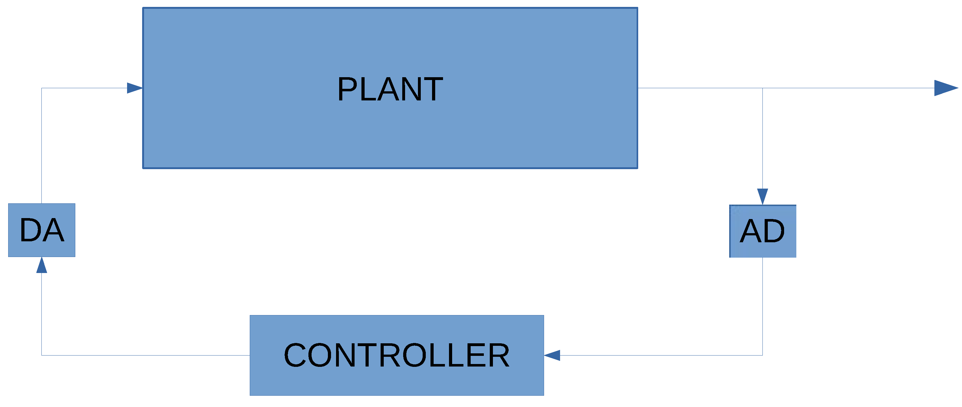
Figure 1. Closed loop composed by plant and controller.
Information 12 00178 g001
Figure 2. Control Software Synthesis Flow.
Information 12 00178 g002
Figure 3. Multi-input Buck DC-DC converter.
Information 12 00178 g003
Figure 4. Picture P for K 1 , as generated by KPS and Gnuplot. The x-axis is in Ampere (A), the y-axis is in Volt (V).
Information 12 00178 g004
Figure 5. Picture C for K 1 , as generated by KPS and Gnuplot. The x-axis represents possible action sets.
Information 12 00178 g005
Figure 6. Picture P for K 2 , as generated by KPS and Gnuplot. The x-axis is in Ampere (A), the y-axis is in Volt (V).
Information 12 00178 g006
Figure 7. Pictures C for K 1 , as generated by KPS and Gnuplot. The x-axis represents possible action sets.
Information 12 00178 g007
Figure 8. Picture P for K 3 , as generated by KPS and Gnuplot. The x-axis is in Ampere (A), the y-axis is in Volt (V).
Information 12 00178 g008
Figure 9. Picture P for K 4 , as generated by KPS and Gnuplot. The x-axis is in Ampere (A), the y-axis is in Volt (V).
Information 12 00178 g009
Table 1. KPS performance (CPU times are in seconds).
aCPU(P)CPU(G) | P | | J | | E |
19.15e+003.25e+026.17e+032.46e+015.19e+03
21.00e+011.47e+031.29e+042.91e+011.09e+04
31.06e+012.43e+031.67e+042.91e+011.39e+04
41.10e+013.58e+032.02e+043.16e+011.68e+04
Publisher’s Note: MDPI stays neutral with regard to jurisdictional claims in published maps and institutional affiliations.