Analysis and Prediction of COVID-19 Using SIR, SEIQR, and Machine Learning Models: Australia, Italy, and UK Cases

Abstract

The novel coronavirus disease, also known as COVID-19, is a disease outbreak that was first identified in Wuhan, a Central Chinese city. In this report, a short analysis focusing on Australia, Italy, and UK is conducted. The analysis includes confirmed and recovered cases and deaths, the growth rate in Australia compared with that in Italy and UK, and the trend of the disease in different Australian regions. Mathematical approaches based on susceptible, infected, and recovered (SIR) cases and susceptible, exposed, infected, quarantined, and recovered (SEIQR) cases models are proposed to predict epidemiology in the above-mentioned countries. Since the performance of the classic forms of SIR and SEIQR depends on parameter settings, some optimization algorithms, namely Broyden–Fletcher–Goldfarb–Shanno (BFGS), conjugate gradients (CG), limited memory bound constrained BFGS (L-BFGS-B), and Nelder–Mead, are proposed to optimize the parameters and the predictive capabilities of the SIR and SEIQR models. The results of the optimized SIR and SEIQR models were compared with those of two well-known machine learning algorithms, i.e., the Prophet algorithm and logistic function. The results demonstrate the different behaviors of these algorithms in different countries as well as the better performance of the improved SIR and SEIQR models. Moreover, the Prophet algorithm was found to provide better prediction performance than the logistic function, as well as better prediction performance for Italy and UK cases than for Australian cases. Therefore, it seems that the Prophet algorithm is suitable for data with an increasing trend in the context of a pandemic. Optimization of SIR and SEIQR model parameters yielded a significant improvement in the prediction accuracy of the models. Despite the availability of several algorithms for trend predictions in this pandemic, there is no single algorithm that would be optimal for all cases.

1. Introduction

In December 2019, the Chinese government informed the rest of the world that a virus was rapidly spreading throughout China. A few months later, it had detrimentally spread to several other countries. The United States Centers for Disease Control and Prevention (CDC) identified a seafood market in Wuhan as the center of the outbreak of the novel coronavirus disease (COVID-19), which is caused by severe acute respiratory syndrome coronavirus 2. The World Health Organization (WHO) reported a case in Thailand on 13 January 2020, the first case to be identified outside China. On 16 January 2020, Japan confirmed its first case of the novel coronavirus, followed by South Korea on 20 January. As of today, most countries around the world have been affected.

Numerous studies have been conducted to predict the spread of the virus in order to seek the best prevention measures. For instance, a simulation model based on mobility data was proposed [1], and a particle swarm optimization (PSO) algorithm was used to estimate the parameters (susceptible, infected, recovered) in the susceptible, infected, and recovered (SIR) cases model [1,2]. The results indicate that the latter method is precise enough, with a low margin of error compared with analytical methods. Another study [3] calibrated the SIR model to South Africa after considering different scenarios for the reproduction number (R0) for reporting infections and short-term healthcare resource estimations. Meanwhile, daily temperature and relative humidity were both reported to influence the occurrence of COVID-19 in Hubei province and some other provinces [4].

The authors of [5] proposed a heuristic algorithm to model and evaluate the risk of the COVID-19 pandemic in six different countries/states, namely New York, California, the whole of the USA, Iran, Sweden, and the UK.

Another work [6] developed two COVID-19 prediction models based on genetic programming and found that both models were highly reliable for prediction of COVID-19 cases in India. The researchers in [7] reviewed the most recent COVID-19 forecasting models and identified the most predominant factors to be hospitalization [8,9,10,11], intensive care units [12,13,14], vaccination [15,16], and age groups [17,18,19].

The first case of COVID-19 in Australia was reported in January 2020. In this paper, we also report on a short analysis focusing on Australia, which continued as a short-term simulation.

The manuscript is organized in several sections. Section 2 presents the research methodology. Section 3 and Section 4 introduce the SIR and susceptible, exposed, infected, quarantined, and recovered (SEIQR) models. Section 5 describes the prediction algorithms (the logistic function and Prophet algorithm). Section 6 provides the results, followed by a discussion and concluding remarks in Section 7.

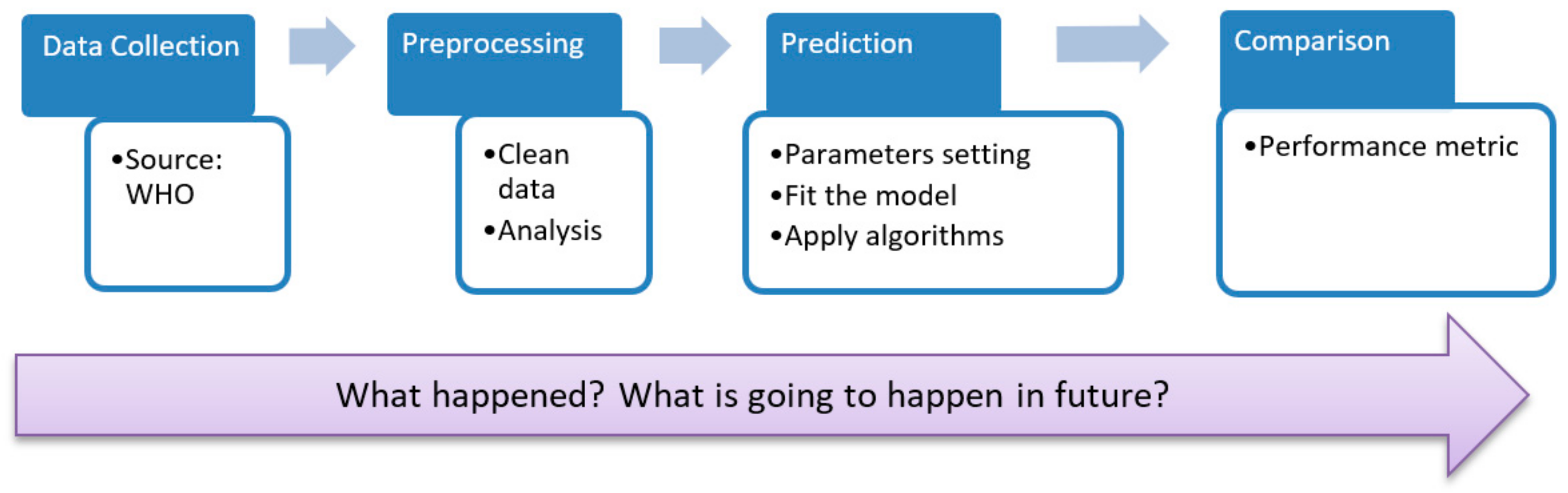
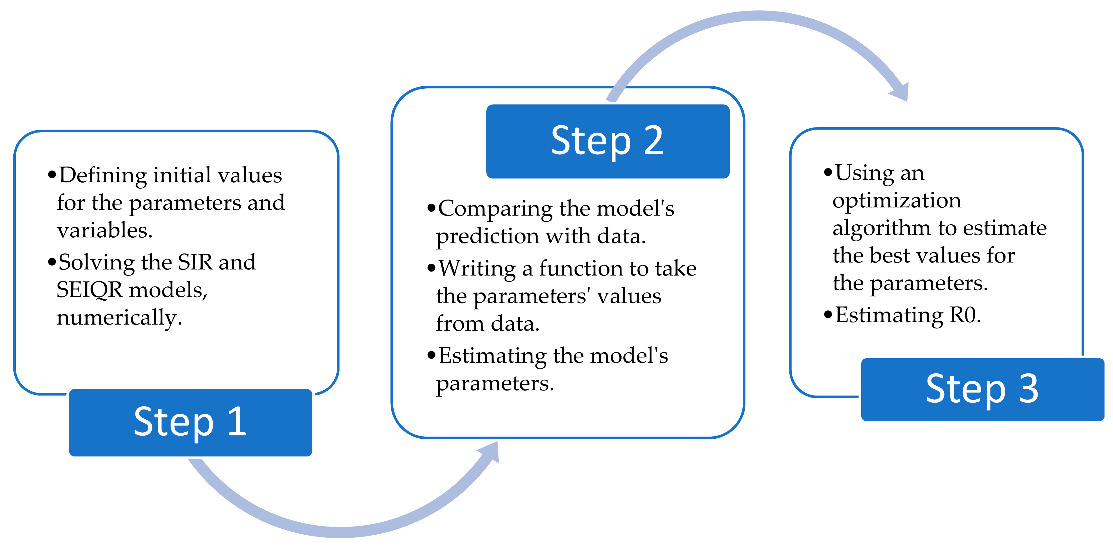
2. Research Methodology

The study was carried out in several phases. First, data were collected from the World Health Organization (WHO) and John Hopkins University, which obtain data from different organizations. After this, the data were analyzed and preprocessed in order to avoid any duplicate or missing values. Numerical tests were performed using Python and R and executed on an Intel^® Core i7-4510U, 2.0 GHz, 8 GB, DDR3 Memory computer (Supplementary File). The flowchart of the research methodology is provided in Figure 1.

Figure 1. Flowchart of the current research process.

3. SIR Model

This section introduces the classic form of the SIR model [20,21], which is used to describe the transmission of COVID-19 in Australia, Italy, and UK. The flowchart of the SIR model is presented in Figure 2.

Figure 2. Susceptible, infected, and recovered (SIR) model.

The SIR model shows how a disease spreads through a population. The equations of the SIR model are as shown below [22]:

$$\frac{ds}{dt}=-\beta IS$$

(1)

$$\frac{dI}{dt}=\beta IS-\gamma I$$

(2)

$$\frac{dR}{dt}=\gamma I$$

(3)

where:

• S is the number of susceptible individuals at time t;
• I is the number of infected individuals at time t;
• R is the number of recovered individuals at time t;
• $\beta$ and $\gamma$ are the transmission rate and rate of recovery (removal), respectively.

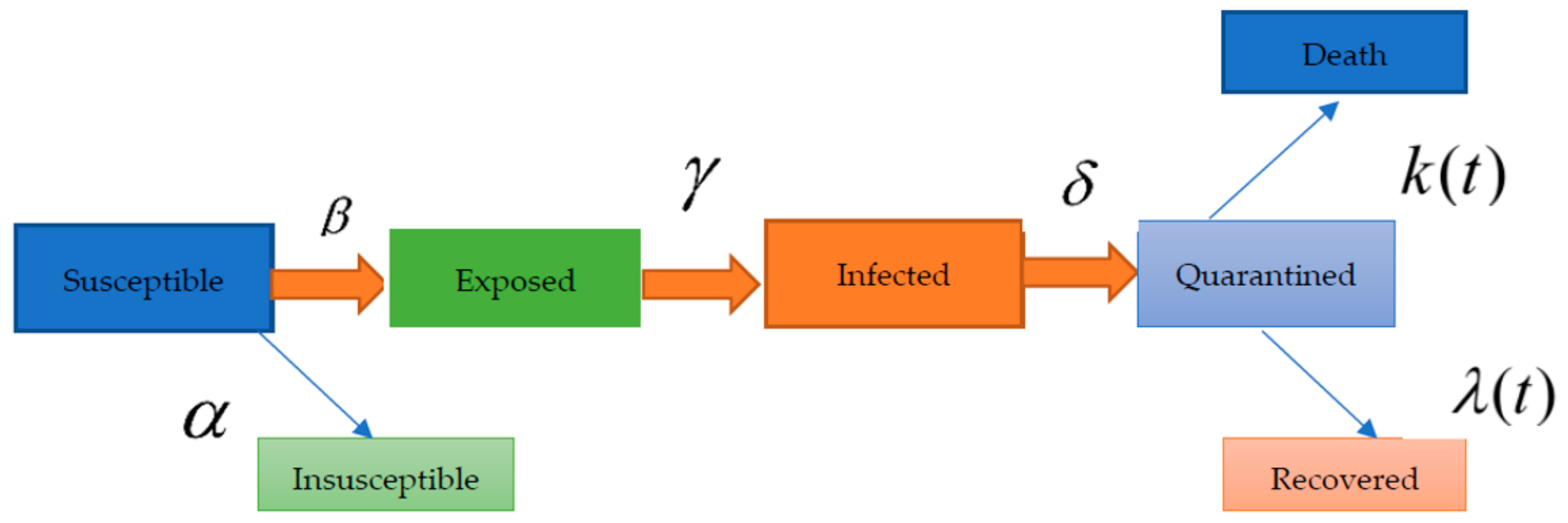
4. SEIQR Model

The SEIQR model, an extended version of SIR [23], models the interaction of people under different conditions: susceptible (S), exposed (E), infected (I), quarantined (Q), and recovered (R). The parameters S, I, and R are the same as those in the SIR model, and E presents the fraction of individuals that have been infected but do not show any signs. The SEIQR model diagram is illustrated in Figure 3.

Figure 3. Susceptible, exposed, infected, quarantined, and recovered (SEIQR) model diagram [23].

The equations of the SEIQR model are defined as follows:

$$\frac{dS(t)}{dt}=-\beta \frac{S(t)I(t)}{N}-\alpha S(t)$$

(4)

$$\frac{dE(t)}{dt}=\beta \frac{S(t)I(t)}{N}-\gamma E(t)$$

(5)

$$\frac{dI(t)}{dt}=\gamma E(t)-\delta I(t)$$

(6)

$$\frac{dQ(t)}{dt}=\delta I(t)-\lambda (t)Q(t)-\kappa (t)Q(t)$$

(7)

$$\frac{dR(t)}{dt}=\lambda (t)Q(t)$$

(8)

$$\frac{dD(t)}{dt}=\kappa (t)Q(t)$$

(9)

$$\frac{dP(t)}{dt}=\alpha S(t)$$

(10)

where $\alpha$ represents the protection rate; $\beta$ is the infection rate and illustrates the inverse of the average latent time; $\gamma$ shows the rate of recovery (removal); $\delta$ represents the inverse of the average quarantine time; ${\lambda }_0 and {\lambda }_1$ are coefficients used in the time-dependent cure rate; ${\kappa }_0 and {\kappa }_1$ are coefficients used in the time-dependent mortality rate [23]; and $\{S(t),P(t),E(t),I(t),Q(t),R(t),D(t)\}$ refer to the susceptible, insusceptible, exposed (infected but not yet infectious, in a latent period), infectious (with infectious capacity and not yet quarantined), quarantined (confirmed and infected), recovered, and closed cases [23].

5. Prediction

The machine learning techniques described in this section were used for COVID-19 case predictions in Australia, Italy, and UK. Machine learning is a branch of computer science in which data teach algorithms, and the learning process is performed as supervised, unsupervised, and/or semi-supervised learning forms [24,25,26,27]. In this section, some approaches that were employed to predict cases (confirmed and deaths) of COVID-19 are discussed.

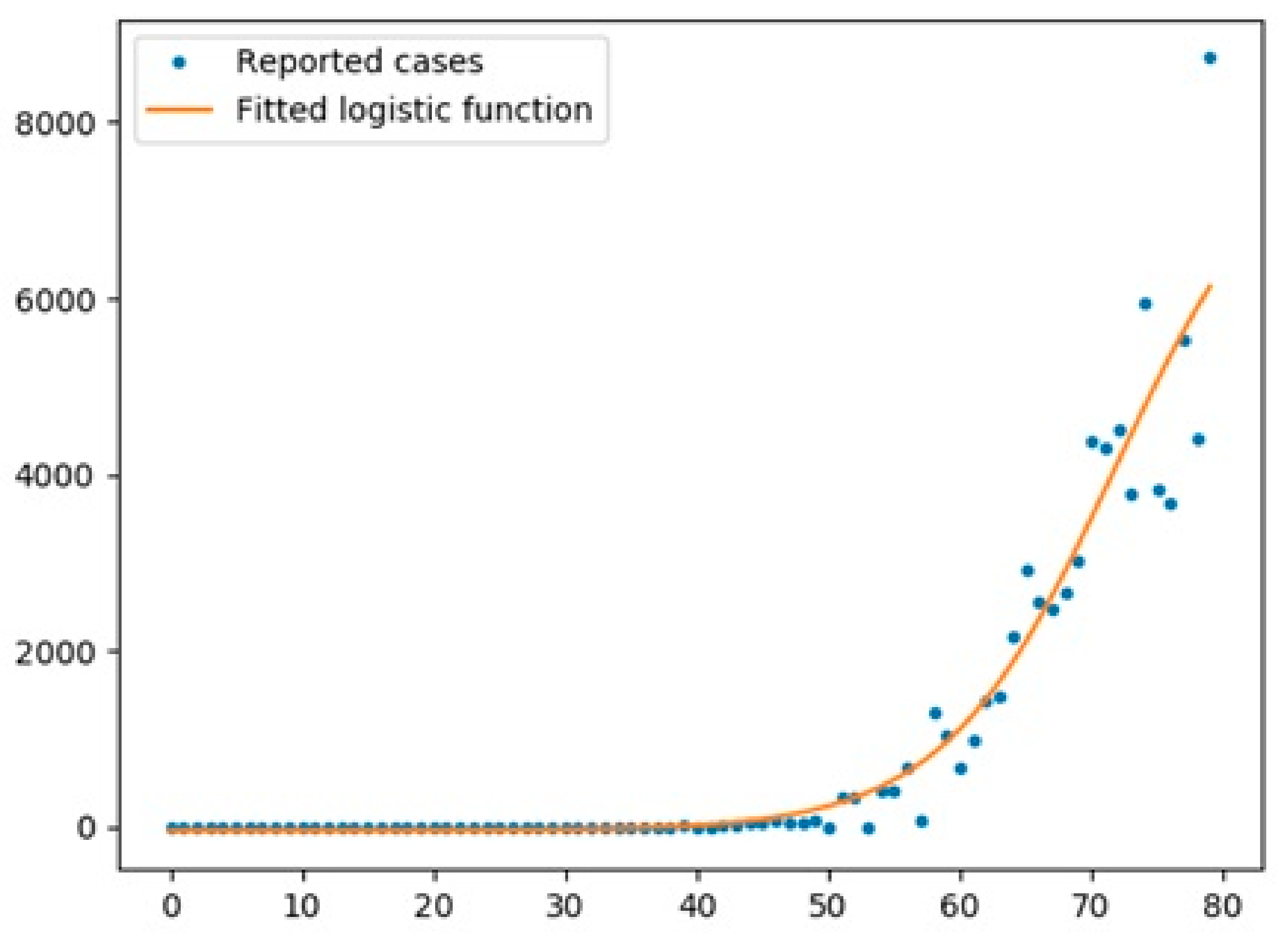
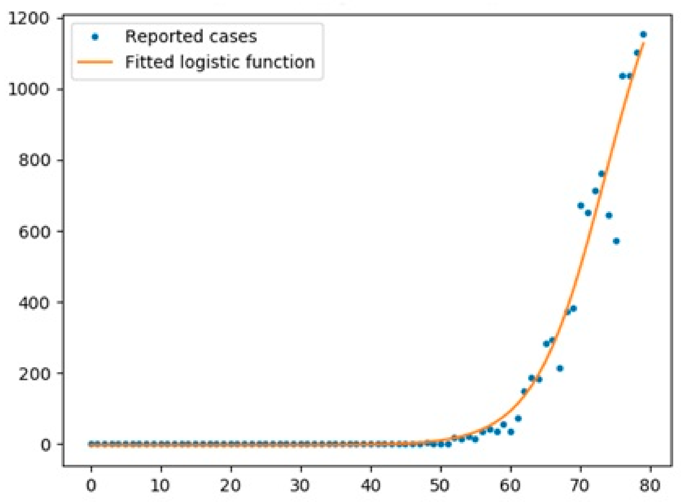
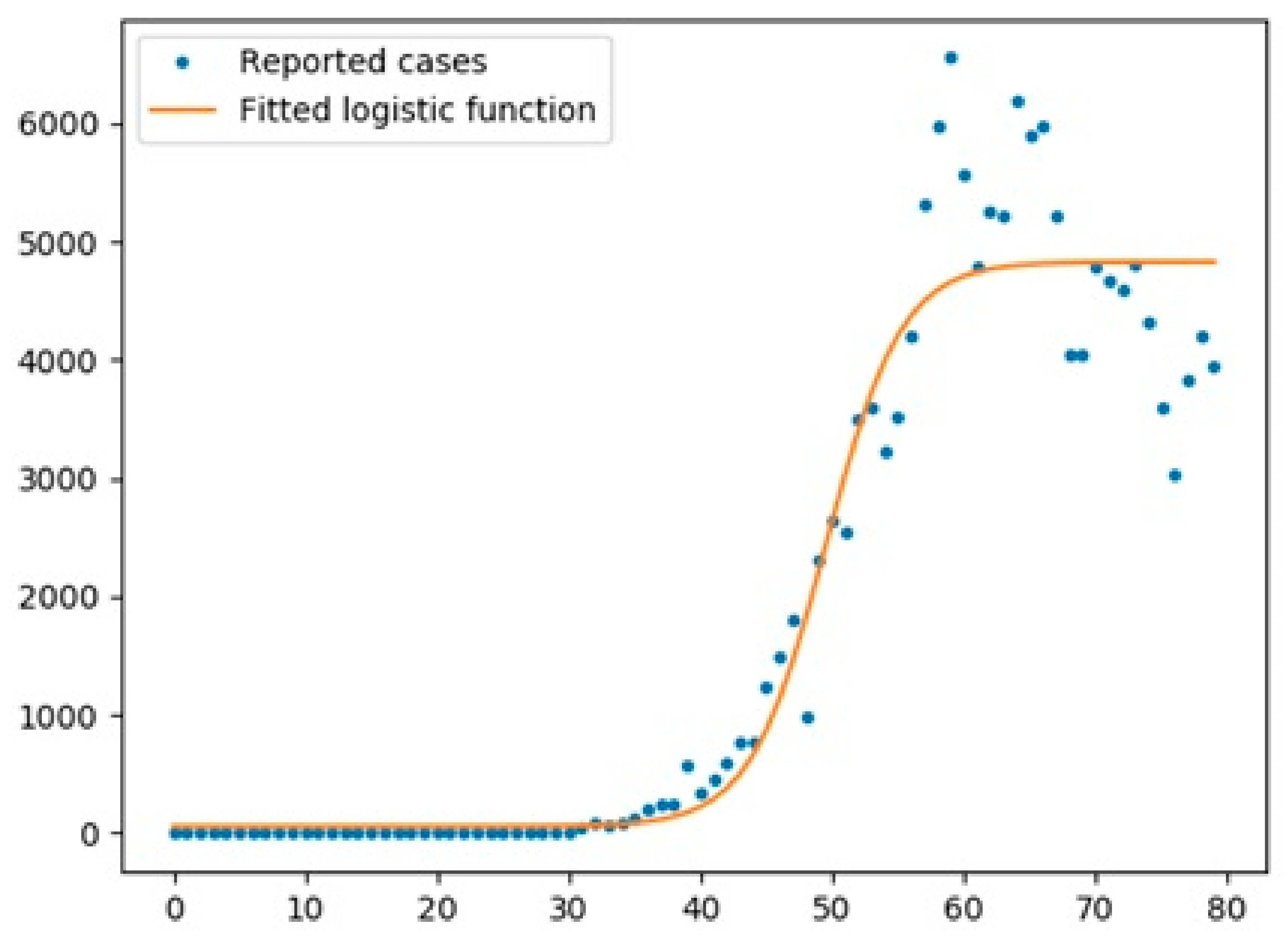
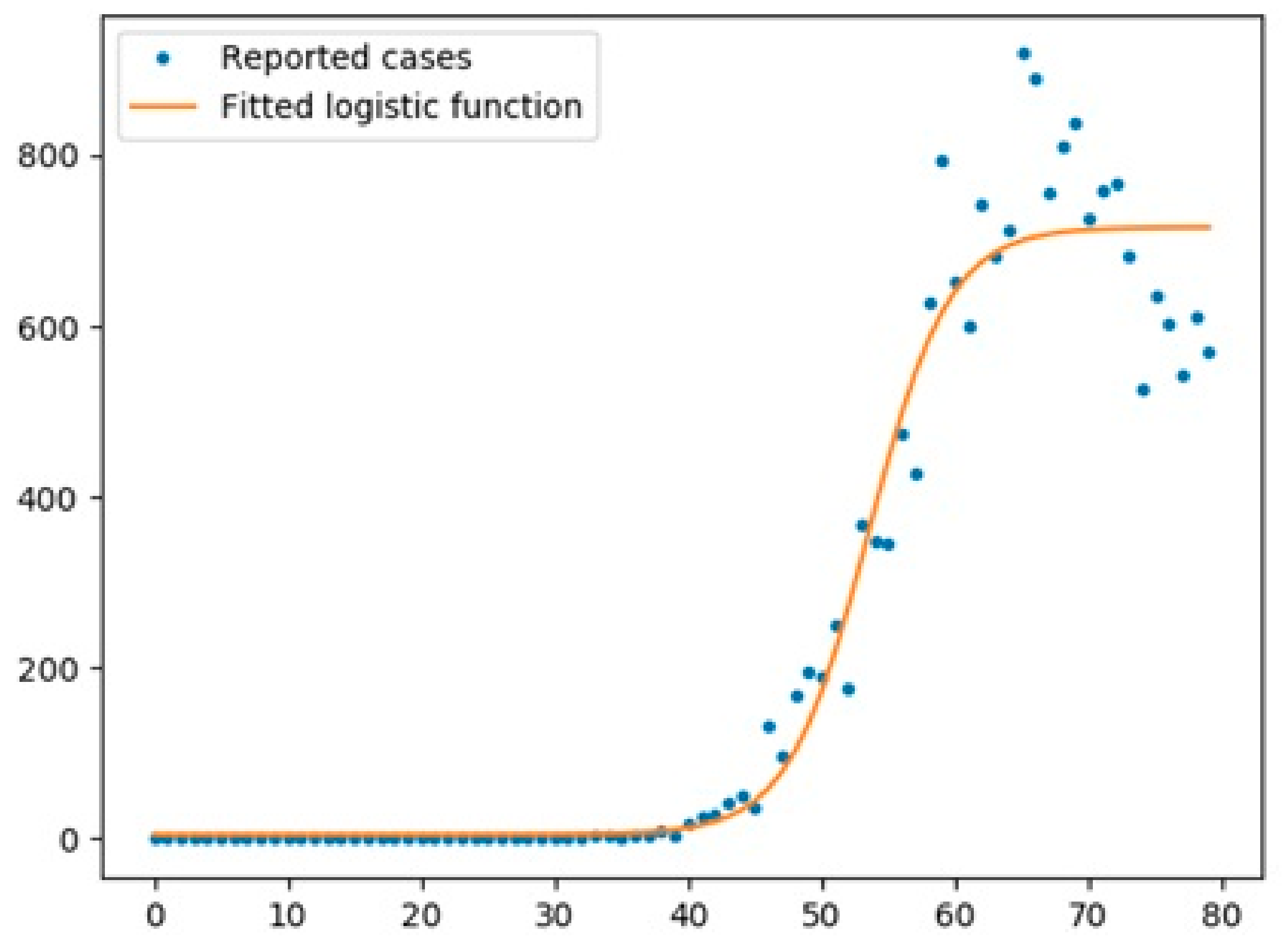
5.1. Logistic Function

A logistic function could be defined as follows:

$$f(x)=\frac{L}{1+e^{-k(x-x_0)}}$$

(11)

where e = Euler’s number, $x_0$ = Sigmoid’s midpoint, L is the curve’s maximum value, and K is the logistic growth of the curve.

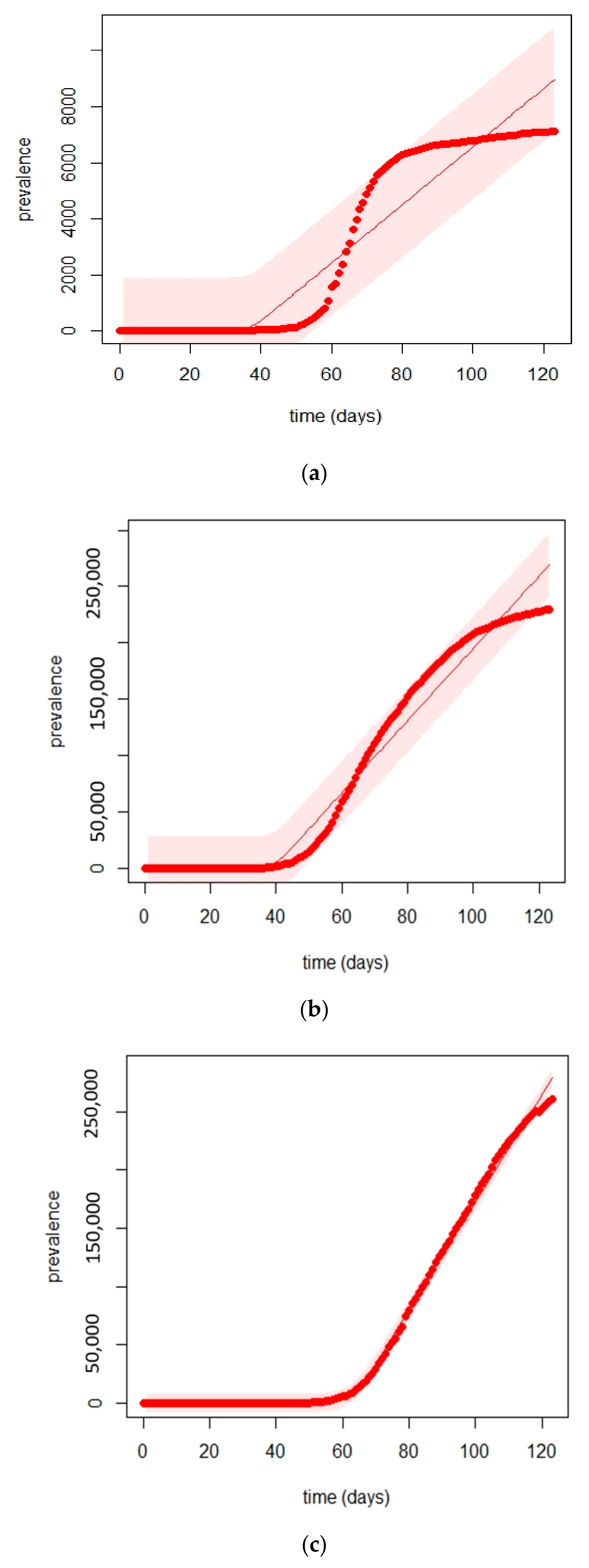
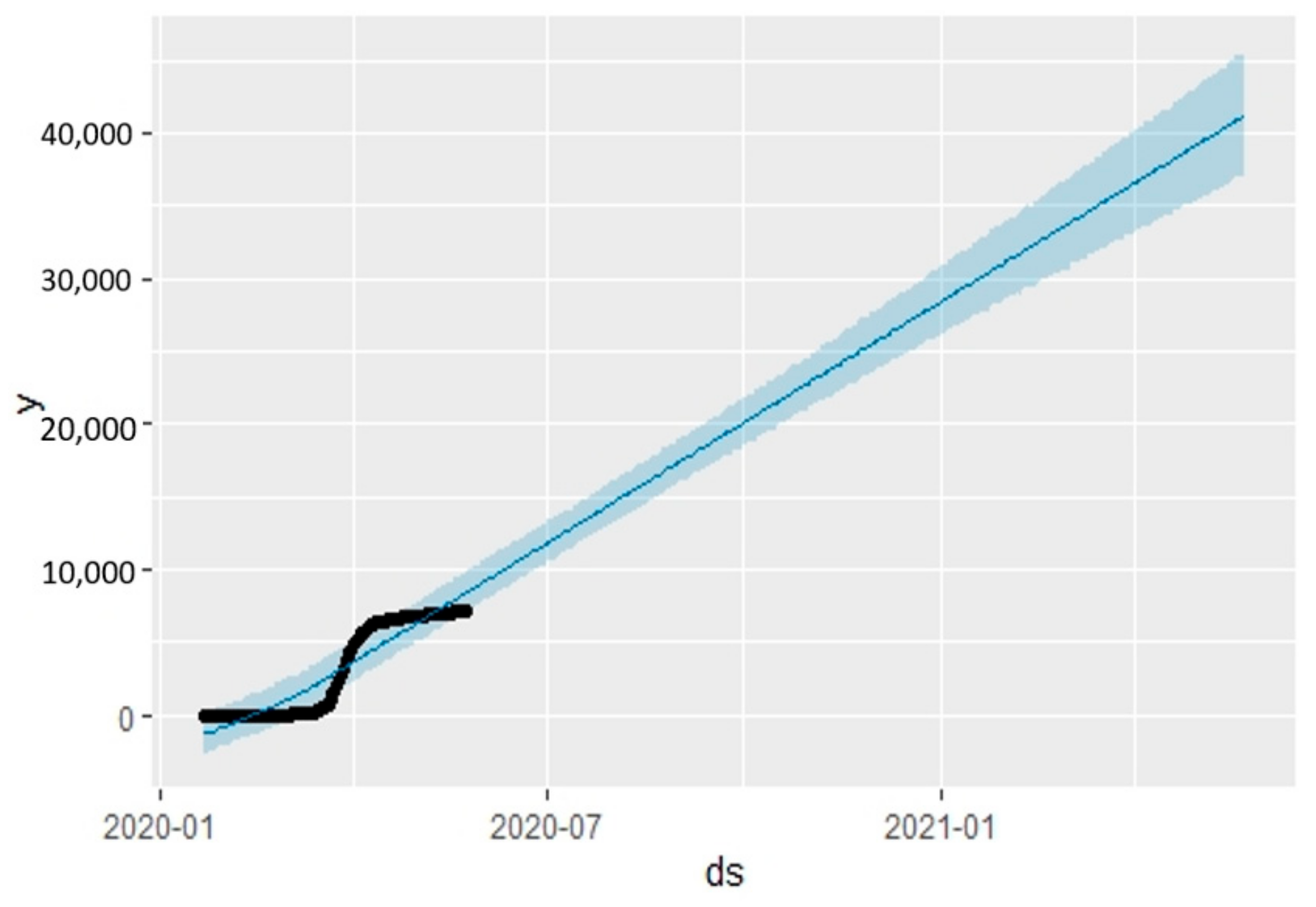
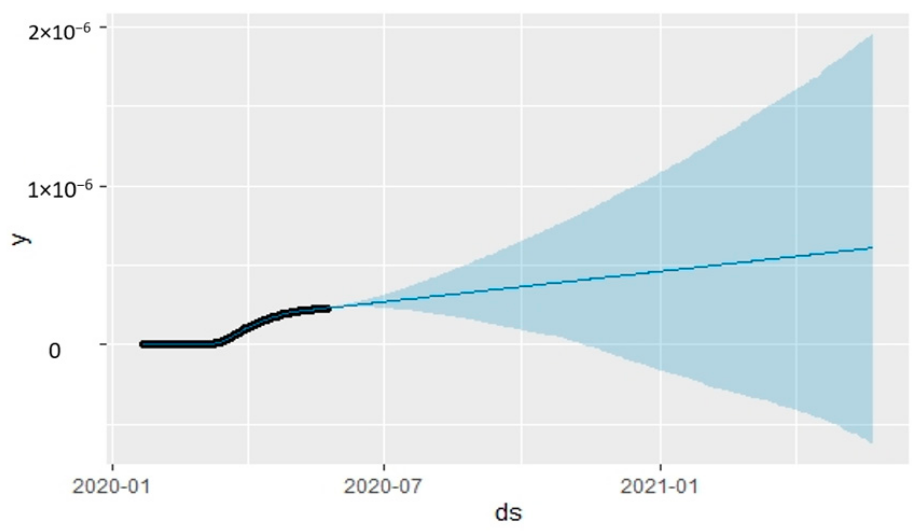
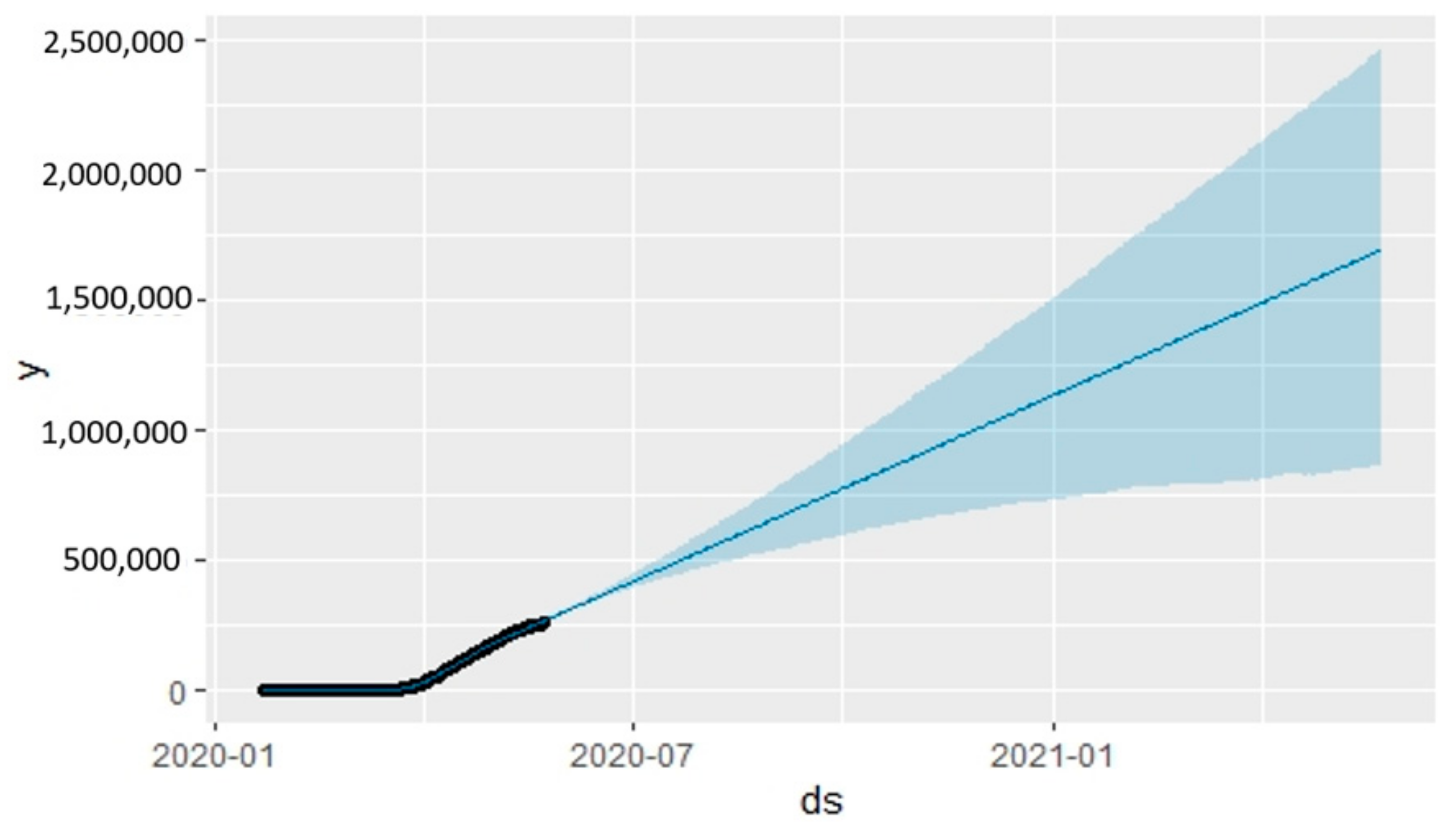
5.2. Times Series Forecasting with the Prophet Algorithm

The Prophet algorithm is an open-source tool developed by Facebook’s Data Science team, which is aimed at business forecasting [28]. This algorithm works well with time-series data that have seasonal effects, and it is robust in dealing with missing data [29]. In the Prophet algorithm, the forecast is determined as follows [29]:

$$\underset{T+h\left|T\right.}{\overset{^}{y}}=\overline{y}=(y_1+y_2+\dots y_T)/T$$

(12)

where $y_1,y_2,\dots ,y_T$ are denoted as historical data; and $\underset{T+h\left|T\right.}{\overset{^}{y}}$ is a short-hand to forecast $\underset{T+h\left|T\right.}{\overset{}{y}}$ based on available data.

6. Results

6.1. Analysis

6.1.1. New Cases

In this subsection, the confirmed growth rates in Australia, Italy, and UK were calculated for every day from 24 April to 23 May 2020. Figure 4 depicts the growth rate of confirmed cases in these countries. As can be seen, the growth rate for Australia remained below 0.5 during times of outbreak and was just above 0.0 at the end of May, while the rates for Italy and UK were generally high. The growth rate for UK was almost above 2.0 in April, and then dramatically declined in May. The rate for Italy fluctuated between 0.5 and 1.5 in April and May.

Figure 4. Growth rate (confirmed cases in Australia, Italy, and UK).

Figure 5 presents the growth rate of death cases for the above-mentioned countries, according to daily data from 24 April to 23 May 2020. The growth rate for death cases in Australia fluctuated between 0.0 and 7.0 in April and May and reached 7.0 at the end of April. During the same period, the rate remained almost below 2.0 in Italy, and in UK, the rate was just below 4.0 at the end of April and just above 0.0 at the end of May.

Figure 5. Growth rate (death cases in Australia, Italy, and UK).

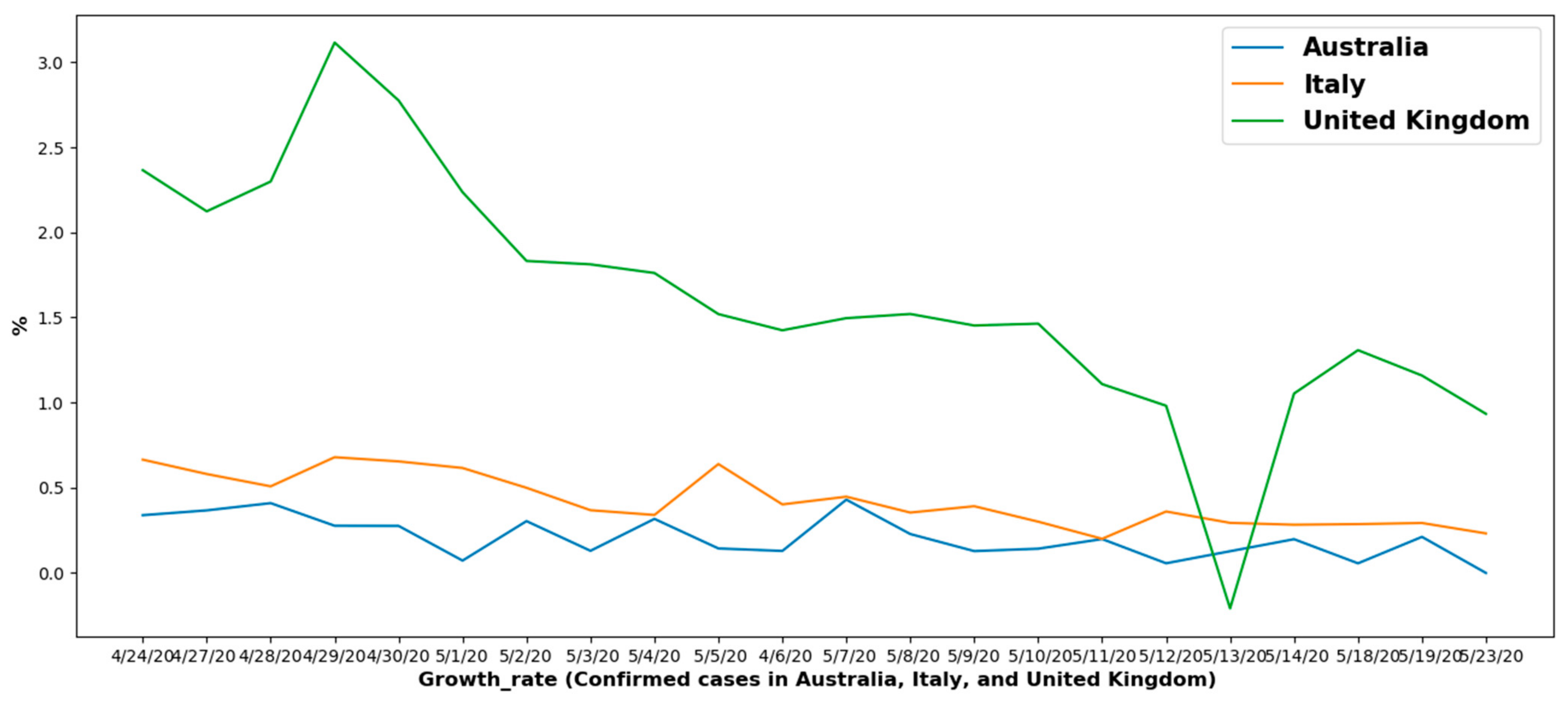
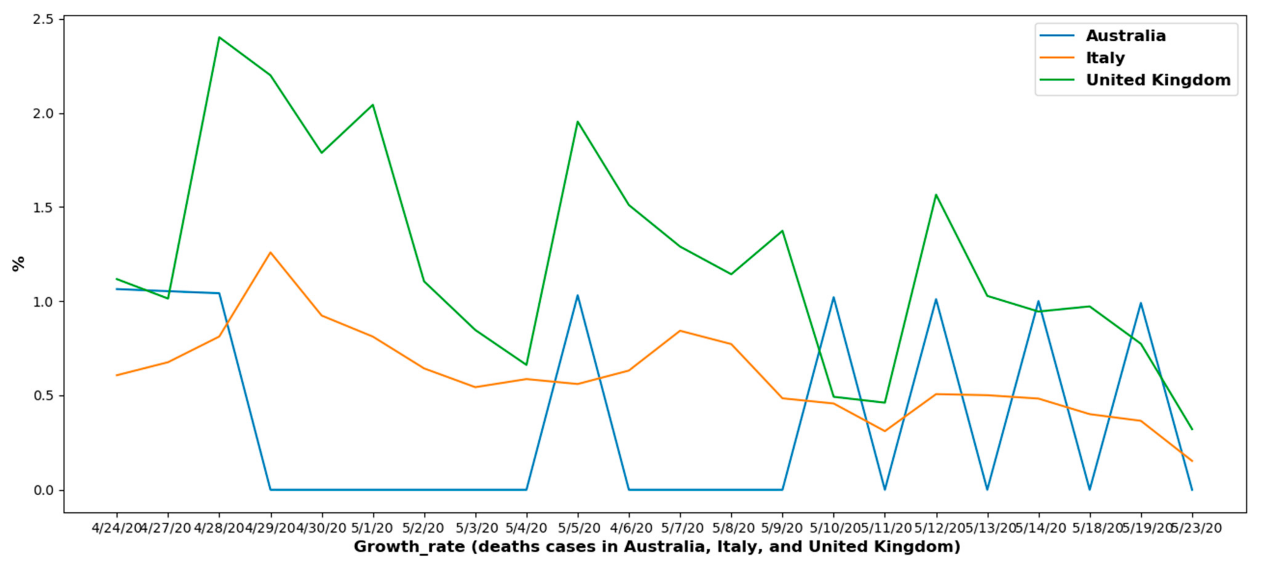
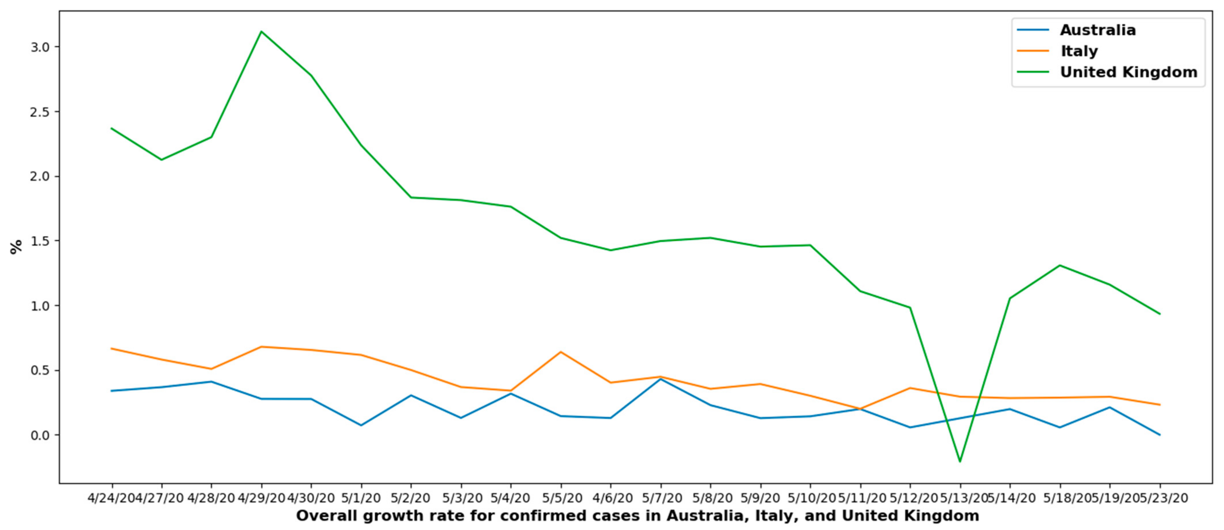
6.1.2. Overall Growth Rate

This section presents the numbers of active cases in these three countries, which were calculated using the following equation:

Active_cases = confirmed_cases − deaths_cases − recovered_cases

(13)

From Equation (13), the overall growth rate could be calculated according to Equation (14), in which i refers to the present day:

Overall growth rate [i] = ((active cases [i] − active case [i-1])/active case [i − 1]) × 100

(14)

Figure 6 illustrates the overall growth rate for confirmed cases in the studied countries. Negative numbers indicate that people recover faster than the rate at which they get sick, which is good news. The rate for Australia in the time period remained almost below zero and then changed from −15 at the end of April to just below −5 at the end of May. For Italy, the rate fluctuated between just above −7.5 and just above 0.0, while the rate for UK remained almost consistently positive in the time horizon (0.0–3.0). Figure 7 illustrates that the number of death cases in Australia is significantly lower than the other two countries.

Figure 6. Overall growth rate for confirmed cases in Australia, Italy, and UK.

Figure 7. Number of death cases in Australia compared with Italy and UK.

Figure 8a–h shows confirmed cases versus death cases in each Australian state. By 23 May 2020, New South Wales and Northern Territory possessed the most confirmed and the least death cases in Australia, respectively. In Figure 8a–h, the number of confirmed and death cases in New South Wales significantly differed from other states in Australia and increased dramatically, while the Northern Territory experienced some fluctuation during the study time period.

Figure 8. Confirmed versus death cases in different Australian states: (a) New South Wales, (b) Australian Capital Territory, (c) Northern Territory, (d) Queensland, (e) South Australia, (f) Tasmania, (g) Victoria, (h) Western Australia.

With the aim of forecasting, the logistic function defined in Equation (11) was applied to the collected data (time horizon: start of outbreak in the countries). According to the results in Figure 9, Figure 10, Figure 11, Figure 12, Figure 13 and Figure 14, the logistic function is fitted to the trend of increasing cases to evaluate the performance of metric R2 scores used for confirmed and death cases. Results are presented in Table 1. The root mean square error (RMSE) was used as another metric to analyze cases, and the results in Table 2 show that the best RMSE value belongs to the Australian cases (confirmed and death).

Figure 9. Prediction of confirmed cases by logistic function (Australia).

Figure 10. Prediction of death cases by logistic function (Australia).

Figure 11. Prediction of confirmed cases by logistic function (UK).

Figure 12. Prediction of death cases by logistic function (UK).

Figure 13. Prediction of confirmed cases by logistic function (Italy).

Figure 14. Prediction of death cases by logistic function (Italy).

Table 1. R2 score for different cases in the three countries.

Country	Confirmed Cases	Death Cases
Australia	0.87	0.67
UK	0.92	0.97
Italy	0.93	0.95

Table 2. Root mean square error (RMSE) values for different cases in the three countries.

Country	Confirmed Cases	Death Cases
Australia	8.22	0.88
UK	21.94	6.97
Italy	23.24	8.00

Figure 15, Figure 16 and Figure 17 present the results of the classic SIR model. As previously mentioned, the controlling $\beta$ parameter indicates the level of disease transmission, and $\gamma$ is the recovery (removal) period indicating how many people could recover in a certain period. First, all parameters were initially added to the SIR model, which was then applied to real data. As can be seen in Figure 15, Figure 16 and Figure 17 and Table 3 (RMSE values), the classic SIR form was not suitable for predicting the COVID-19 pandemic in these three countries. In order to fit the SIR model to Australia, Italy, and UK, an optimizer was needed to find the unknown parameters ($\beta$ and $\gamma$) from equation $R_0$($R_0=\frac{\beta }{\gamma }$) since these parameters could be estimated. Prior to the outbreak in these countries, it is essential to address whether the number of susceptible cases is equal to the population due to the absence of antibodies and vaccines for the disease. At first, $R_0$ = 2.7 was fixed (reported by Australian Government: Department of Health) as the median number, $\beta =0.378$, and $\gamma =0.14$.

Figure 15. Predicted cases in Australia using the susceptible, infected, recovered (SIR) model (blue: real confirmed cases; red: SIR model).

Figure 16. Predicted cases in Italy based on the SIR model (blue: real confirmed cases; red: SIR model).

Figure 17. Predicted cases in UK based on the SIR model (blue: real confirmed cases; red: SIR model).

Table 3. RMSE values obtained by SIR model (before optimization of parameters).

Italy	UK	Australia
18.75	15.45	831.84

Real data were applied to estimate the values of $\beta$ and $\gamma$. An optimizer was used to find the best estimation of $\beta$ and $\gamma$. The optimization algorithms used were the Broyden–Fletcher–Goldfarb–Shanno (BFGS) [30], limited memory bound constrained BFGS ( L-BFGS-B) [31], conjugate gradients (CG) [30], and Nelder–Mead algorithms [32]. The parameter settings are provided in Table 3. The flowchart of the improved SIR and SEIQR versions and parameter settings for the above-mentioned algorithms are addressed in Figure 18 and Table 4, respectively.

Figure 18. Flowchart of improved versions of SIR and SEIQR models.

Table 4. Parameter settings.

Algorithm	Parameter Setting
BFGS	Maxit = 100, reltol * = 10−8
Nelder–Mead	Maxit = 500, reltol = 10−8, alpha = 1, beta = 0.5, gamma = 2.0
L-BFGS-B	Maxit = 100, reltol = 10−8, lmm ** = 5, factr *** = 107
CG	Maxit = 100, reltol = 10−8

* Reltol = Relative convergence tolerance, ** lmm = number of BFGS updates retained, *** factr = convergence factor, e = Euler’s number.

Table 5 provides the optimized values obtained by different algorithms (SIR model). The best values for the parameters were found using the Nelder–Mead algorithm (for the SIR model) and L-BFGS-B algorithm (for the SEIQR model). This method is illustrated in Figure 18. As previously mentioned, before the start of the outbreak, the number of susceptible cases was equal to the populations of these countries, since neither antibodies nor a developed vaccine were available. According to Wikipedia, the populations of Australia, Italy, and UK were 25⁰⁶, 60⁰⁶, and 67⁰⁶, respectively. Table 6 illustrates the RMSE values obtained by the algorithms (for SIR and SEIQR models), showing improvements in significantly reducing the values. Figure 19a–c presents the confirmed cases provided by the optimized SEIQR model with the above-mentioned descriptions in the three countries (see Figure 18).

Table 5. Median values of SIR parameters determined by the Department of Health in each country.

Country	$\mathit{\beta }$				$\mathit{\gamma }$				${\mathit{R}}_0$
Algorithm	BFGS	Nelder–Mead	L-BFGS-B	CG	BFGS	Nelder–Mead	L-BFGS-B	CG	BFGS	Nelder–Mead	L-BFGS-B	CG
Australia	0.014	0.014	0.378	0.37	0.22	0.22	0.14	0.14	0.063	0.063	2.64	2.64
UK	0.37	3.84701−3	0.37	0.37	0.14	1.94−1	0.14	0.14	2.64	0.02	2.64	2.64
Italy	0.37	1.083555−3	0.37	0.37	0.14	3.9088−1	0.14	0.37	2.64	0.01	2.64	2.64

Table 6. RMSE values obtained based on the improved SIR model considering a 0.99 confidence interval.

Model	Italy	UK	Australia
SIR model	1.41	1.01	1.13
SEIR model	1.12	1.23	1.04

Figure 19. Prediction by optimized SEIQR model for: (a) Australia, (b) Italy, and (c) UK.

Figure 20, Figure 21 and Figure 22 reveal the forecasted values obtained using the Prophet algorithm, where the algorithm is fitted for the cases of Italy and UK but has errors for Australia. Table 7, Table 8 and Table 9 present the results of the predicted cumulative confirmed cases using the Prophet algorithm in the three countries, where y represents the true values of confirmed cases, ds is time, $\hat{y}$ is the forecasted values, and $\widehat{y_{lower}}$ and $\widehat{y_{upper}}$ are the lower and upper bounds for the forecasted values, respectively. It should be noted that the forecasted values were determined between the cutoff and cutoff + horizon. Table 7, Table 8 and Table 9 are also cross-validation matrices that are used to find the error values between y and $\hat{y}$, from which the RMSE values can be obtained (Figure 23a–c).

Figure 20. Forecasting by Prophet algorithm for the next year (confirmed cases in Australia).

Figure 21. Forecasting by Prophet algorithm for the next year (confirmed cases in Italy).

Figure 22. Forecasting by Prophet algorithm for the next year (confirmed cases in UK).

Table 7. Predicted cumulative confirmed cases in Australia (cross-validation matrix).

y	ds	$\hat{\mathit{y}}$	$\widehat{{\mathit{y}}_{\mathit{l}\mathit{o}\mathit{w}\mathit{e}\mathit{r}}}$	$\widehat{{\mathit{y}}_{\mathit{u}\mathit{p}\mathit{p}\mathit{e}\mathit{r}}}$	Cutoff
7095	21 May 2020	21,309.752	18,998.140	23,829.955	4 April 2020
7099	22 May 2020	21,630.708	19,245.072	24,269.904	4 April 2020
7114	23 May 2020	21,959.985	19,424.097	24,640.939	4 April 2020
7114	24 May 2020	22,326.688	19,766.194	25,093.353	4 April 2020

Table 8. Predicted cumulative confirmed cases in UK (cross-validation matrix).

y	ds	$\hat{\mathit{y}}$	$\widehat{{\mathit{y}}_{\mathit{l}\mathit{o}\mathit{w}\mathit{e}\mathit{r}}}$	$\widehat{{\mathit{y}}_{\mathit{u}\mathit{p}\mathit{p}\mathit{e}\mathit{r}}}$	Cutoff
252,246	21 May 2020	143,776.53	126,702.28	162,413.93	4 April 2020
255,544	22 May 2020	146,462.83	128,526.68	165,539.80	4 April 2020
258,504	23 May 2020	148,818.88	130,813.85	168,216.41	4 April 2020
260,916	24 May 2020	150,344.39	131,476.87	170,004.00	4 April 2020

Table 9. Predicted cumulative confirmed cases in Italy (cross-validation matrix).

y	ds	$\hat{\mathit{y}}$	$\widehat{{\mathit{y}}_{\mathit{l}\mathit{o}\mathit{w}\mathit{e}\mathit{r}}}$	$\widehat{{\mathit{y}}_{\mathit{u}\mathit{p}\mathit{p}\mathit{e}\mathit{r}}}$	Cutoff
228,006	21 May 2020	373,982.5	336,940.1	415,612.7	4 April 2020
228,658	22 May 2020	379,300.7	340,862.6	422,338.4	4 April 2020
229,327	23 May 2020	384,792.4	344,957.8	429,120.3	4 April 2020
229,858	24 May 2020	390,481.8	349,482.8	436,663.2	4 April 2020

Figure 23. Visualization of performance metric for Prophet algorithm (considering RMSE) for (a) UK, (b) Australia, and (c) Italy.

7. Discussion and Conclusions

COVID-19 is a family of coronaviruses that has affected the lives of billions of people worldwide. The first section of this paper presented a short analysis of COVID-19, focusing on its effect in Australia, Italy, and UK. Specifically, the analysis gives a comparison of the confirmed cases and death rates between Australia, Italy, and UK and among the different states of Australia. The analysis reveals that Australia is in a generally good position compared with the other two countries. However, the situation in different regions of Australia is rather complicated. For example, New South Wales has the most confirmed cases and death cases, while Northern Territory shows the least confirmed and death cases (it is worth mentioning that New South Wales has a larger population).

Mathematical approaches based on SIR and SEIQR were proposed to predict the epidemiology in Australia, Italy, and UK. Since the classic forms of SIR and SEIQR are deterministic, an improved version based on parameter optimization is suggested to improve the prediction. The results were compared with the logistic function and Prophet algorithm, and are summarized as follows:

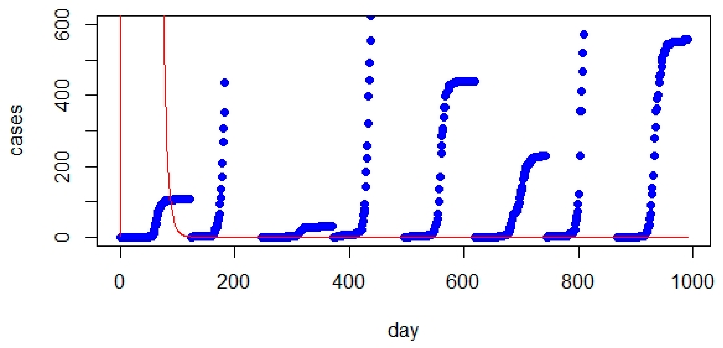
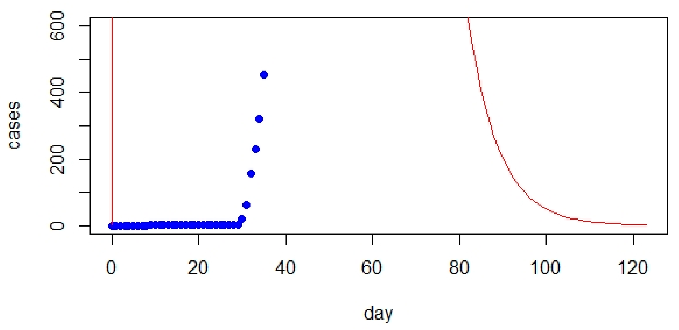
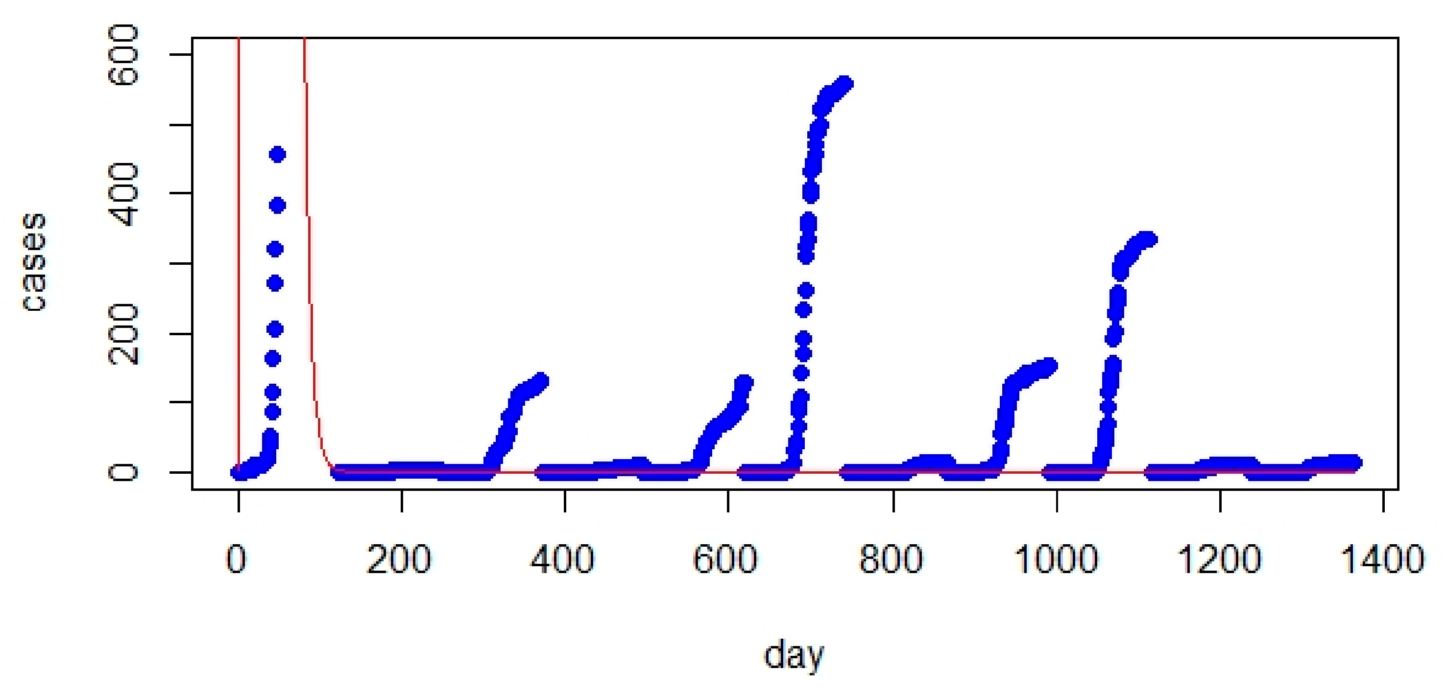
• The comparison between the classic SIR model and real data showed a significant gap. However, initializing the parameters of the SIR model significantly improved the prediction.
• The classic SIR model worked best for UK but was not suitable for Australia based on RMSE values.
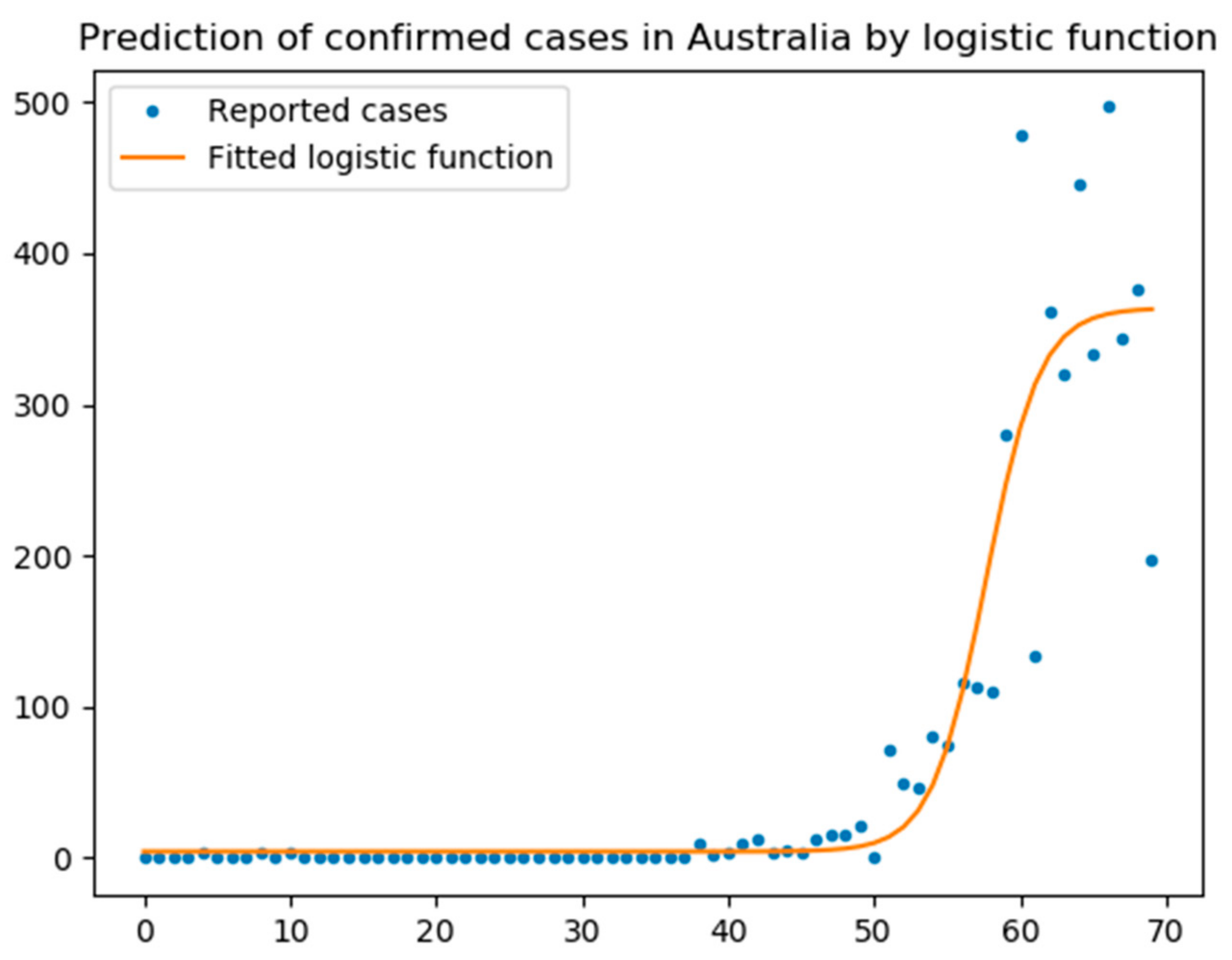
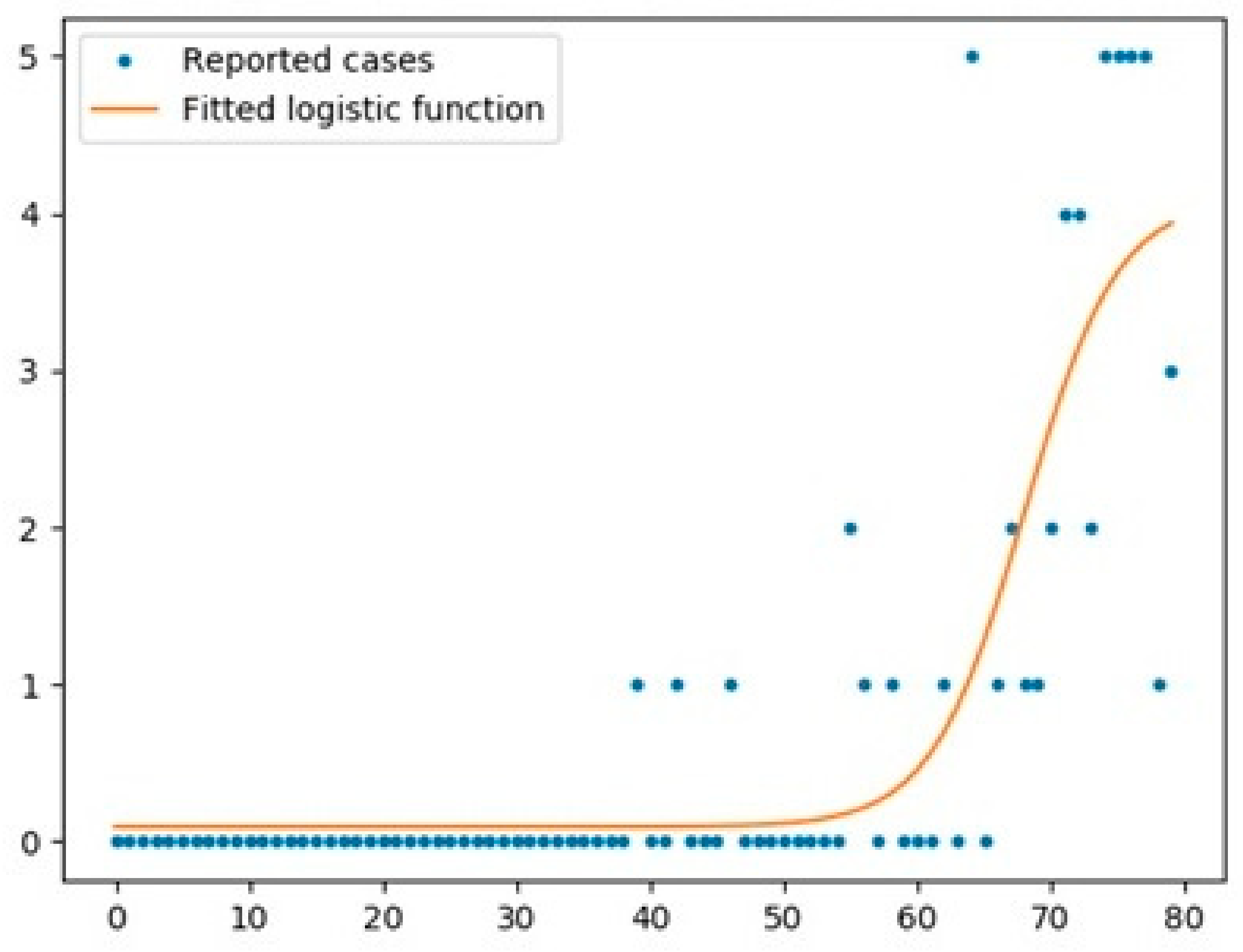
• The logistic function was a good model for UK with an R2 score of 0.97, while the scores for Australia and Italy were 0.67 and 0.95, respectively.
• The best RMSE value belonged to the Australian cases (confirmed and deaths).
• Parameter optimization for the SIR and SEIQR models significantly improved their prediction accuracy.
• The improved version of SEIQR exhibited better performance than the SIR model (regarding RMSE values and figures).
• The optimized SEIQR model has better prediction for UK and Italy compared with Australia.
• The best values for the parameters were determined using the Nelder–Mead algorithm for the SIR model and the L-BFGS-B algorithm for the SEIQR model.
• The Prophet algorithm worked better for Italy and UK cases than for Australian cases.
• The logistic function had a better performance for cases in all three countries compared with the Prophet algorithm.
• The improved versions of the SIR and SEIQR models exhibited a better performance than the logistic function, Prophet algorithm, and classic SIR model.

Some studies and research on related viruses have predicted that COVID-19 is dependent on environmental characteristics and will decline with higher temperature, humidity, ultraviolet (UV) light [33], and with spatial colony-growth heterogeneity [34]. Since UV light has been strongly associated with lower COVID-19 growth, projections suggest that, without intervention, COVID-19 will decrease temporarily during summer, rebound by autumn, and peak the subsequent winter. Regarding the above-mentioned discussion, the growth rate appears to be a country-specific characteristic.

The evolution of COVID-19 throughout the world is difficult to predict. Until a reliable vaccine becomes available for all, which may only happen by the end of 2021, governments will have to strike the tough balance between health and other issues, such as economic and social. Although social distancing costs an economic and psychological price, recent experience in several countries indicates that lifting a majority of restrictions increases the potential for multiple local outbreaks (second and third waves). In the absence of an effective and reliable vaccine, preparedness for this “wave” phenomenon is absolutely required.

One limitation of this study is that the authors did not account for human behavior or control measures in the models. By modeling the maximum growth rate and using a threshold number of cases, we could restrict the analyses to the period during which the disease expanded quickly: between the beginning of community transmission and the implementation of major control measures. This aspect alone is a suggested direction for further study.

Another limitation of this paper is the untimely analysis, which was an analysis based on data retrieved up until May 2020. If we look at the current data, the trend of COVID-19 cases is completely different from the predictions made in this paper. However, the results of this paper show that the growth rate is a country-specific characteristic and depends on time. Some factors relevant to these country specifications are the country’s size, population heterogeneity factor, etc. A similar effect of heterogeneous subpopulations is that, for instance, they are known for spreading bacterial colonies. Furthermore, there exist much more advanced models for the COVID-19 pandemic, whereby the inclusion of hospitalization rates, use of intensive care units (ICUs), and age groups is influential (vaccinations will be included in this list in the near future). All the above-mentioned issues are encouraged for future studies.

In addition, all the forecasting in this paper was addressed without considering the scenario of social distancing and quarantine, which is valuable as a future research direction. While this paper analyzes the improved SIR and SEIQR models, it would be interesting to test other epidemiology models. Moreover, it would be worthwhile to combine mathematical models with other observations, such as policy interventions, human behavior, and constraints, which may yield better prediction performance.

References

- Aràndiga, F.; Baeza, A.; Cordero-Carrión, I.; Donat, R.; Martí, M.C.; Mulet, P.; Yanez, D.F. A Spatial-Temporal Model for the Evolution of the COVID-19 Pandemic in Spain Including Mobility. Mathematics 2020, 8, 1677. [Google Scholar] [CrossRef]
- Putra, S.; Mu’tamar, Z.K. Estimation of Parameters in the SIR Epidemic Model Using Particle Swarm Optimization. Am. J. Math. Comput. Model. 2019, 4, 83–93. [Google Scholar] [CrossRef]
- Mbuvha, R.R.; Marwala, T. On Data-Driven Management of the COVID-19 Outbreak in South Africa. medRxiv 2020. [Google Scholar] [CrossRef]
- Qi, H.; Xiao, S.; Shi, R.; Ward, M.P.; Chen, Y.; Tu, W.; Su, Q.; Wang, W.; Wang, X.; Zhang, Z. COVID-19 transmission in Mainland China is associated with temperature and humidity: A time-series analysis. Sci. Total Environ. 2020, 728, 138778. [Google Scholar] [CrossRef]
- Asteris, P.G.; Douvika, M.G.; Karamani, C.A.; Skentou, A.D.; Chlichlia, K.; Cavaleri, L.; Daras, T.; Armaghani, D.J.; Zaoutis, T.E. A Novel Heuristic Algorithm for the Modeling and Risk Assessment of the COVID-19 Pandemic Phenomenon. Comput. Model. Eng. Sci. 2020, 125, 815–828. [Google Scholar] [CrossRef]
- Salgotra, R.; Gandomi, M.; Gandomi, A.H. Time Series Analysis and Forecast of the COVID-19 Pandemic in India using Genetic Programming. Chaos Solitons Fractals 2020, 138, 109945. [Google Scholar] [CrossRef] [PubMed]
- Rahimi, I.; Chen, F.; Gandomi, A.H. A review on COVID-19 forecasting models. Neural Comput. Appl. 2021, 1–11. [Google Scholar] [CrossRef]
- Reno, C.; Lenzi, J.; Navarra, A.; Barelli, E.; Gori, D.; Lanza, A.; Valentini, R.; Tang, B.; Fantini, M.P. Forecasting COVID-19-Associated Hospitalizations under Different Levels of Social Distancing in Lombardy and Emilia-Romagna, Northern Italy: Results from an Extended SEIR Compartmental Model. J. Clin. Med. 2020, 9, 1492. [Google Scholar] [CrossRef] [PubMed]
- Santosh, K.C. COVID-19 Prediction Models and Unexploited Data. J. Med. Syst. 2020, 44, 1–4. [Google Scholar] [CrossRef]
- Putra, M.; Kesavan, M.M.; Brackney, K.; Hackney, D.N.; Roosa, M.K.M. Forecasting the impact of coronavirus disease during delivery hospitalization: An aid for resource utilization. Am. J. Obstet. Gynecol. MFM 2020, 2, 100127. [Google Scholar] [CrossRef] [PubMed]
- Nabi, K.N. Forecasting COVID-19 pandemic: A data-driven analysis. Chaos Solitons Fractals 2020, 139, 110046. [Google Scholar] [CrossRef]
- Fenga, L. Forecasting the COVID-19 Diffusion in Italy and the Related Occupancy of Intensive Care Units. J. Probab. Stat. 2021, 2021, 1–9. [Google Scholar] [CrossRef]
- Gaglione, D.; Braca, P.; Millefiori, L.M.; Soldi, G.; Forti, N.; Marano, S.; Willett, P.K.; Pattipati, K.R. Adaptive Bayesian Learning and Forecasting of Epidemic Evolution—Data Analysis of the COVID-19 Outbreak. IEEE Access 2020, 8, 175244–175264. [Google Scholar] [CrossRef]
- Berta, P.; Lovaglio, P.G.; Paruolo, P.; Verzillo, S. Real Time Forecasting of Covid-19 Intensive Care Units Demand; Publications Office of the European Union: Luxembourg, 2020. [Google Scholar]
- Dean, N.E.; Piontti, A.P.Y.; Madewell, Z.J.; Cummings, D.A.; Hitchings, M.D.; Joshi, K.; Kahn, R.; Vespignani, A.; Halloran, M.E.; Longini, I.M. Ensemble forecast modeling for the design of COVID-19 vaccine efficacy trials. Vaccine 2020, 38, 7213–7216. [Google Scholar] [CrossRef]
- Kane, P.B.; Moyer, H.; MacPherson, A.; Papenburg, J.; Ward, B.J.; Broomell, S.B.; Kimmelman, J. Expert Forecasts of COVID-19 Vaccine Development Timelines. J. Gen. Intern. Med. 2020, 35, 3753–3755. [Google Scholar] [CrossRef]
- Keeling, M.J.; Hill, E.M.; Gorsich, E.E.; Penman, B.; Guyver-Fletcher, G.; Holmes, A.; Leng, T.; McKimm, H.; Tamborrino, M.; Dyson, L.; et al. Predictions of COVID-19 dynamics in the UK: Short-term forecasting and analysis of potential exit strategies. PLoS Comput. Biol. 2021, 17, e1008619. [Google Scholar] [CrossRef] [PubMed]
- Brand, S.P.C.; Aziza, R.; Kombe, I.K.; Agoti, C.N.; Hilton, J.; Rock, K.S.; Parisi, A.; Nokes, D.J.; Keeling, M.J.; Barasa, E.W. Forecasting the scale of the COVID-19 epidemic in Kenya. MedRxiv 2020. [Google Scholar] [CrossRef]
- Massonnaud, C.; Roux, J.; Crépey, P. COVID-19: Forecasting short term hospital needs in France. medrxiv 2020. [Google Scholar] [CrossRef]
- Kermack, W.O.; McKendrick, A.G. Contributions to the mathematical theory of epidemics—II. The problem of endemicity. Bull. Math. Biol. 1991, 53, 57–87. [Google Scholar] [CrossRef]
- Capasso, V.; Serio, G. A generalization of the Kermack-McKendrick deterministic epidemic model. Math. Biosci. 1978, 42, 43–61. [Google Scholar] [CrossRef]
- Weiss, H.H. The SIR model and the foundations of public health. Mater. Mat. 2013, 2013, 1–17. [Google Scholar]
- Peng, L.; Yang, W.; Zhang, D.; Zhuge, C.; Hong, L. Epidemic analysis of COVID-19 in China by dynamical modeling. arXiv 2020, arXiv:2002.06563. [Google Scholar]
- Mitchell, T.M. Machine learning and data mining. Commun. ACM 1999, 42, 30–36. [Google Scholar] [CrossRef]
- Arkes, H.R. Overconfidence in Judgmental Forecasting. In Harvey J. Greenberg; Springer International Publishing: Berlin/Heidelberg, Germany, 2001; pp. 495–515. [Google Scholar]
- Armstrong, J.S. Standards and Practices for Forecasting. In Harvey J. Greenberg; Springer International Publishing: Berlin/Heidelberg, Germany, 2001; pp. 679–732. [Google Scholar]
- Maleki, M.; Mahmoudi, M.R.; Wraith, D.; Pho, K.-H. Time series modelling to forecast the confirmed and recovered cases of COVID-19. Travel Med. Infect. Dis. 2020, 37, 101742. [Google Scholar] [CrossRef]
- Taylor, S.J.; Letham, B. Forecasting at Scale. Am. Stat. 2018, 72, 37–45. [Google Scholar] [CrossRef]
- Ndiaye, B.M.; Tendeng, L.; Seck, D. Analysis of the COVID-19 pandemic by SIR model and machine learning technics for forecasting. arXiv 2020, arXiv:2004.01574v1. [Google Scholar]
- Chambers, L.G.; Fletcher, R. Practical Methods of Optimization. Math. Gaz. 2001, 85, 562. [Google Scholar] [CrossRef]
- Byrd, R.H.; Lu, P.; Nocedal, J.; Zhu, C. A Limited Memory Algorithm for Bound Constrained Optimization. SIAM J. Sci. Comput. 1995, 16, 1190–1208. [Google Scholar] [CrossRef]
- Nelder, J.A.; Mead, R. A Simplex Method for Function Minimization. Comput. J. 1965, 7, 308–313. [Google Scholar] [CrossRef]
- Merow, C.; Urban, M.C. Seasonality and uncertainty in global COVID-19 growth rates. Proc. Natl. Acad. Sci. USA 2020, 117, 27456–27464. [Google Scholar] [CrossRef] [PubMed]
- Kindler, O.; Pulkkinen, O.; Cherstvy, A.G.; Metzler, R. Burst statistics in an early biofilm quorum sensing model: The role of spatial colony-growth heterogeneity. Sci. Rep. 2019, 9, 1–19. [Google Scholar] [CrossRef] [PubMed]
Publisher’s Note: MDPI stays neutral with regard to jurisdictional claims in published maps and institutional affiliations. |
© 2021 by the authors. Licensee MDPI, Basel, Switzerland. This article is an open access article distributed under the terms and conditions of the Creative Commons Attribution (CC BY) license (http://creativecommons.org/licenses/by/4.0/).