Article

Fall Detection from Electrocardiogram (ECG) Signals and Classification by Deep Transfer Learning

by
Fatima Sajid Butt
1,*,
Luigi La Blunda
1,
Matthias F. Wagner
1,
Jörg Schäfer
1,
Inmaculada Medina-Bulo
2 and
David Gómez-Ullate
2
1
Computer Science and Engineering, Frankfurt University of Applied Sciences, D-60318 Frankfurt am Main, Germany
2
Escuela Superior de Ingeniería, Universidad de Cádiz, 11001 Cádiz, Spain
*
Author to whom correspondence should be addressed.
Information 2021, 12(2), 63; https://doi.org/10.3390/info12020063
Submission received: 15 December 2020 / Revised: 27 January 2021 / Accepted: 28 January 2021 / Published: 3 February 2021
(This article belongs to the Special Issue Computer Vision for Biomedical Image Applications)

Abstract

:
Fall is a prominent issue due to its severe consequences both physically and mentally. Fall detection and prevention is a critical area of research because it can help elderly people to depend less on caregivers and allow them to live and move more independently. Using electrocardiograms (ECG) signals independently for fall detection and activity classification is a novel approach used in this paper. An algorithm has been proposed which uses pre-trained convolutional neural networks AlexNet and GoogLeNet as a classifier between the fall and no fall scenarios using electrocardiogram signals. The ECGs for both falling and no falling cases were obtained as part of the study using eight volunteers. The signals are pre-processed using an elliptical filter for signal noises such as baseline wander and power-line interface. As feature extractors, frequency-time representations (scalograms) were obtained by applying a continuous wavelet transform on the filtered ECG signals. These scalograms were used as inputs to the neural network and a significant validation accuracy of 98.08% was achieved in the first model. The trained model is able to distinguish ECGs with a fall activity from an ECG with a no fall activity with an accuracy of 98.02%. For the verification of the robustness of the proposed algorithm, our experimental dataset was augmented by adding two different publicly available datasets to it. The second model can classify fall, daily activities and no activities with an accuracy of 98.44%. These models were developed by transfer learning from the domain of real images to the medical images. In comparison to traditional deep learning approaches, the transfer learning not only avoids “reinventing the wheel,” but also presents a lightweight solution to otherwise computationally heavy problems.

1. Introduction

The World Health Organization (WHO) defines fall as “unintentionally coming to the ground or some lower level and other than as a consequence of sustaining a violent blow, loss of consciousness, sudden onset of paralysis as in stroke or an epileptic seizure” [1].
According to a study, falls are the dominant cause of unintentional injury-related deaths and non-fatal injuries in people aged 65 and above. It poses a severe challenge for senior adults and people with movement disabilities [2]. The likelihood of falls increases with age and diminished health quality of an individual. The frequency of falls is more significant in seniors living in nursing homes than those who are living in an outside community. According to [3], approximately 30–50% of people residing in long-term care institutions fall per annum, and 40% of them experience repetitive falls. About two-thirds of people who suffer a fall are susceptible to recurrent falls. About 50% of the patients who lay on the floor for more than an hour after a fall died within six months of the fall [4].
A critical step in providing timely responses to falls is detecting them as early as possible. Several studies and surveys have been conducted to categorize falls and detect them.
In this study we aimed to detect human activities, in particular fall events using wearable devices based on electrocardiograms (ECG) sensor data. To this end, we classified the activities with a pre-trained deep neural network; i.e., we applied a transfer learning approach to reduce training time and data.
The paper is structured as follows: A brief description of the technologies used in our study is given in Section 2. Section 3 presents an overview of the different forms of fall detecting techniques and human activity recognition (HAR) in the literature along with an emphasis on our contribution to the field. The experimental setup and data collection process are illustrated in Section 4. Section 5 presents our proposed methodology and explains the algorithms used. It also describes the phases of our work and its implementation. Section 6 reviews the collected results and their implications. This leads to the discussion related to our research question in Section 7. Finally, Section 8 outlines the conclusion and gives some future perspectives that can be used to further probe the field of HAR using ECG signals.

2. Background

For the reader’s convenience, we briefly explain the technologies that were employed in this section.
Several fall detection systems exist in literature. A recent review of the fall detection systems in [5] categorizes them as follows: (i) wearable devices, (ii) ambient systems, (iii) image processing systems and (iv) combined systems. Wearable devices provide a cheaper and more practical solution in terms of freedom of movement and energy consumption. The aim of most fall detection systems is not only to detect a fall but also to inform concerned authorities in case of an urgent medical emergency. Most of the latest algorithms for fall detection use machine learning [6] and deep learning algorithms [7].
Deep learning became prominent in computer vision (CV) when a deep learning convolution neural network, AlexNet, outperformed its competitors in the ImageNet Large-Scale Visual Recognition Challenge (ILSVRC) in 2012 during an image classification task. Before the wide spread recognition of deep learning, features from the data had to be hand crafted and then fed into a machine learning model. Deep learning in general and convolutional neural networks (CNNs) in particular, have revolutionized the field by not only detecting the features themselves but the features selected by them have been proven to be more significant than those crafted by hand [8].
According to [9], “transfer learning is a machine learning method where a learning model developed for a first learning task is reused as the starting point for a learning model in a second learning task.”
It can also be defined as the ability of a system to recognize and apply knowledge and skills learned in previous domains/tasks to novel domains/tasks, which share some commonality [10]. Transfer learning has been formally defined and categorized in [10]. The problem statement, notation and definition used here are also taken from [10]. A domain D is comprised of two components: a feature space X and a marginal probability P ( X ) , where X = { x 1 , x 2 , x n } X . Similarly, given a specific domain, D = { X , P ( X ) } , a task consists of two components: a label space Y and an objective predictive function f ( · ) (denoted by T = { Y , f ( · ) } ), which is not observed but can be learned from the training data, which consist of pairs { x i , y i } , where x i X and y i Y . The function f ( · ) can be used to predict the corresponding label, f ( x ) , of a new instance x. From a probabilistic viewpoint, f(x) can be written as P ( Y | X ) .
Formally transfer learning is defined as, “Given a source domain D S and learning task T S , a target domain D T and learning task T T , transfer learning aims to help improve the learning of the target predictive function f T (.) in D T using the knowledge in D S and T S , where D S D T , or T S T T .”
Transferring knowledge from one domain to another using transfer learning is not only of theoretical interest, but also of great practical importance, as it can spare a lot of training time and resources and by reducing the data necessary in a domain, it can make learning feasible at all. In our work we have transferred the knowledge gained from training neural networks with natural images to the domain of synthetic, artificial medical images in order to classify images, that were created as a result of pre-processing medical data such as ECG data.

3. Related Work and Our Contribution

This section reviews the work that has been previously done to detect falls using different methods and highlights our contribution to the field. Many surveys and reviews, such as [11,12,13], exist in literature which describe different fall detection techniques, standard experimental protocols for fall simulations and their relative advantages and disadvantages. Detecting fall comes under the vast umbrella of human activity recognition (HAR). HAR is usually considered a computer vision (CV) problem where CV algorithms are used on images or videos to distinguish one activity from another. However, other device-free solutions based on, e.g., radio signals, such as received signal strength (RSSI) or channel state information (CSI) exist; see, e.g., [14,15,16]. Alternatively, wearable sensors provide a resource friendly and practical solution to real time activity recognition, e.g., in particular the rising popularity of gadgets such as smartwatches is an indicator for this trend. Many studies like [17,18] infuse readings from accelerometers and ECG sensors at decision level to determine an activity. Though the wavelet transform has been previously used for analyzing ECG signals for detecting different cardiac conditions as reviewed in [19], it has never been used separately to differentiate a fall from non-fall. Similarly [20] analyzes the impact of body movements on ambulatory ECG frequency spectrum. It also uses artificial neural networks to classify different body movements.
The ECG signals predict the overall health of the human body. A considerable amount of effort has already been contributed to the area of fall detection using accelerometers and gyroscopes. Some studies, such as that in [21], have used different machine learning techniques on these sensor readings to predict and detect the fall. Few studies use ECG signals to predict the falls like in [22], but our study uses the frequency-time domain of the ECG signals by computing their continuous wavelet transform (CWT) coefficients and converting them into scalograms. The overall idea is mainly inspired by [23] where a convolutional neural network (CNN) has been trained on scalograms to differentiate between different heart diseases using ECG signals. Similar approach was used in our study to differentiate between falls and no-falls ECG signals.
The CNN we utilize has also been used in [24] to extract features for bio-metric purposes using gait features from sensor data. However, in our work, for the first time we classify the following activities using ECG signals: Fall, Resting, and general Daily Activities, i.e., we distinguish not only Fall from Resting but also Fall from Daily Activities, where Daily Activities refer to generic daily activities performed by the subjects. The fall risk using heart rate variability in combination with data mining techniques is assessed in [25].
In this paper, we have tried to explore the research question, “Can a fall be detected by using only ECG signals?” by collecting the ECG signals of people falling and then applying our proposed algorithm on the signals. The purpose of this study is to use the biomedical electrical signals of the heart via electrocardiogram to train a deep neural network to analyze and observe the patterns of ECG before and during the fall. Although a lot of work has already been done to detect falls using accelerometers and gyroscopes along with heart rate variability, the focus of this study has been to use ECG as the only factor to determine the presence of fall. Here we are not referring to the cases where cause of the fall is due to a specific heart condition.
This study has explored the less studied field of ECG signals for fall detection by applying machine learning techniques in it. It is based partially on [26] but extends the results obtained therein substantially.
In the field of medical imaging, finding an appropriate amount of data has always been a challenge. That is mainly due to two reasons: Firstly, because of strict data privacy issues, and secondly, finding a large group of volunteers for conducting experiments can be challenging. A data augmentation technique for time series called slicing was used to enhance the limited dataset.
For the machine learning domain, we used transfer learning and compared two of the popular pre-trained networks for image classification—AlexNet and GoogLeNet. We have demonstrated that it could be really beneficial to use a pre-trained network in medical imaging domain as it does not require a lot of data. However, we would like to emphasize that it is an initial study with a focus on the proof of concept in a laboratory set up. It is not conclusive enough to be deployed but it does provide a strong baseline for further workt.

4. Experimental Setup and Data Collection

There are some online ECG databases available like ECGVIEW [27] and physionet [28] which provide ECGs for different research purposes. The ECG databases for people falling could not be found so the ECG data was collected as part of the experiment. The data acquisition system consisted of two components: a hardware component which was obtained from [29] and a software component; for the system architecture we refer to Figure 1.
The hardware component consisted of a wearable belt with ECG sensor attached to a Arduino board. The wearable prototype was designed after taking several features in account as explained in [31]. The device should have been able to record the signals continuously and should be adaptable to the experiment protocol which requires a lot of movement including falls. For this reason, a 3-lead ECG was opted as it is not only a standard for emergency purposes (e.g., in ambulance) but it also requires less wiring and hence provides patient compliance. The readings of a 3-lead ECG are comparable to a 12-lead ECG in our experimental set up. The design of the wearable device is discussed in detail in [31].
Out of many different types of falls, rolling-out-bed as a main and significant one was chosen for this study. Rolling out is defined as from lying, rolling out of bed and going to the floor [21]. The experimental setup consisted of a bed or a table. The sensor and Arduino gadget were worn by the subject. The ECG electrodes were tapped on the chest of the subject. Then the Bluetooth low energy (BLE) connection between the peripheral and central device was established.

4.1. Inclusion Criteria

The study was administered on 8 healthy subjects out of which 3 were females and 5 were males. The mean age of the subjects was 34.5. The following inclusion criteria were designed to enlist the volunteers for the HAR experiment:
  • Age between 18 and 55 years.
  • No history of heart disease or hypertension.
  • No drugs or alcohol consumption before the experiment.
  • No physical constraints for falling (arthritis, etc.).
Our experiment was evaluated by the security officer of our university and a risk assessment was established with assistance from a medical doctor classifying our study as a HAR experiment in accordance with the ethical principles of the Declaration of Helsinki [32].
The heart of a human goes through various changes from birth to adulthood. ECG parameters vary for different age groups in general below 18. Human heart goes through a lot of physiological and anatomical changes from birth to adolescence. This causes some ECG features to differ significantly in adults as compared to children of different ages [33]. In order to correctly interpret the results with various age groups in children, one should have detailed knowledge of age dependant changes which is out of scope for our study. That is the reason the age group chosen was between 18 and 55 for the experiment.

4.2. The HAR Experiment

The ECG was recorded in three positions: laying down, falling by rolling over from the bed and performing daily activities (such as walking and running). Figure 2 shows the fall in three steps. The first on the extreme left is resting position. Next comes the fall initiation and it ends with the person laying on the ground without moving.
Each experiment lasted about a total of 40–45 min consisting of multiple sub-readings of 30 s each. A total of three falls was recorded in a single reading. In each fall, the subject was in resting position as shown in the Figure 2 for first 10 s. In the next 10 s, the volunteers would fall by rolling off the side of the table/bed and would lay on the ground until 30 s are completed. Then the subject would go up and repeat. A similar protocol was used by [34], a prominent dataset for falls and activities of daily life. The laying down or resting period after fall may indicate subconsciousness after fall and hence is necessary to include when designing a fall protocol mimicking elderly population. Some elderly people do not move after the fall. According to [35], a study conducted on 110 participants, of the 60% who fell, 80% were unable to get up after at least one fall and 30% had lain on the floor for an hour or more. According to [36], inactivity after the activity is a common basis for determination of a fall situation. Each reading consisted of 90 s containing a fall every 30 s. On average, 10 readings from each subject were collected.
For the resting ECG, the subject had to lay down on a flat surface without talking and moving to avoid the muscle noise. The log file consisting of 90 s for fall and 30 s for Resting was sent to the central device via BLE. For daily activities, subjects performed some tasks like walking in a fast pace, sitting and standing for an average time of 10 to 15 s following no specific pre-determined protocol.

4.3. The Collected Data

The data collected consists of a total of 8 volunteers. Readings from two of the volunteers were too distorted to be used so they were not included in the next steps. In literature, one would find many HAR experiments which have been conducted using a limited number of volunteers. The benchmark HAR dataset Opportunity [37] used in [38] consists of readings from 4 participants. Similarly, other datasets like PAMAP2 [39] and Skoda [40], which have been used in [41], used 9 and 1 participants respectively for data collection. It is important to note that since it is a preliminary study, more experiments are planned and recommended for future work including elder people and people with some pre-existing heart issues. An overall summary of the collected data is presented in Table 1. This table presents the data statistics as it was collected and saved in files. Due to limited time with each volunteer, some of the subjects performed only fall experiments, others could do only resting readings and some could perform all three including daily activities. Table 2 presents the overview of multiple data instances that were obtained from those files.

5. Our Methodology and Implementation Protocol

The following section outlines our proposed algorithm and its initial implementation.

5.1. Proposed Algorithm

The basic Algorithm 1 designed involves the following steps:
1.
Pre-processing.
2.
Filtering.
3.
Calculating the continuous wavelet transform and creating scalograms.
4.
Fine tuning and retraining a pre-trained CNN.
5.
CNN Classification.
Algorithm 1 Detecting fall with raw ECG signals
Input: A time series ECG raw data Ts
Output: The classified activity label l
T s E C G _ R A W _ V A L U E _ E X T R A C T I O N ( T s )
T s F I L T E R ( T s )
W T S S C A L O G R A M _ C R E A T I O N ( T s )
l C N N _ C L A S S I F I C A T I O N ( W T S )
E C G _ R A W _ V A L U E _ E X T R A C T I O N ( T s ) includes pre-processing raw ECG signals by performing an Analog to Digital Conversion (ADC), i.e., extracting the voltage from the raw data, observing the frequency domain and if required, interpolating the data to upsample to ensure uniform sampling frequency. F I L T E R ( T s ) applies elliptical filtering to remove noisy artifacts from raw ECG signals T s . After the signals have been filtered, wavelet transform is calculated for each signal. The absolute value of wavelet transform is used to create corresponding scalograms or scale-frequency images. The set of images is fed into a fine tuned pre-trained convolutional neural network. Algorithm 2 describes the algorithm for using AlexNet for classification. The trained model is then verified using k-fold verification.
Algorithm 2 CNN_CLASSIFICATION
Input: A set of Frequency-scale Scalograms W T S
Output: The classified activity label l
A l e x N e t R E T R A I N _ F I N E _ T U N E D _ A L E X N E T
l A l e x N e t ( W T S )
returnl

5.2. ECG Signal Filtering

ECG is a low amplitude bio-signal that can be easily contaminated by several different types of artifacts and other bio-signals. A lot of sensor-related information or overhead has to be removed from the log file at the initial stages of filtration.
The sensor value we get is value from an analog to digital 14 bit converter (ADC). The following formula was used to find the corresponding voltage to the ADC value [42]:
V o l t a g e = 3.3 V 16 , 385 × A D C R e a d i n g
Noises in ECG signal are composed of components at high–frequency and/or at low–frequency. Noises with high–frequency components include power line interface, muscle noise and white Gaussian noise. Baseline wandering is a noise with low–frequency components. Minimizing baselines wander and power line interference is the first step in all electrocardiograph (ECG) signal processing [43]. Major noise artifacts lie in the following regions [44]:
  • Muscle noise—5–50 Hz.
  • External electrical noises—50 or 60 Hz.
  • Respiration Noise—0.12–0.5 Hz.
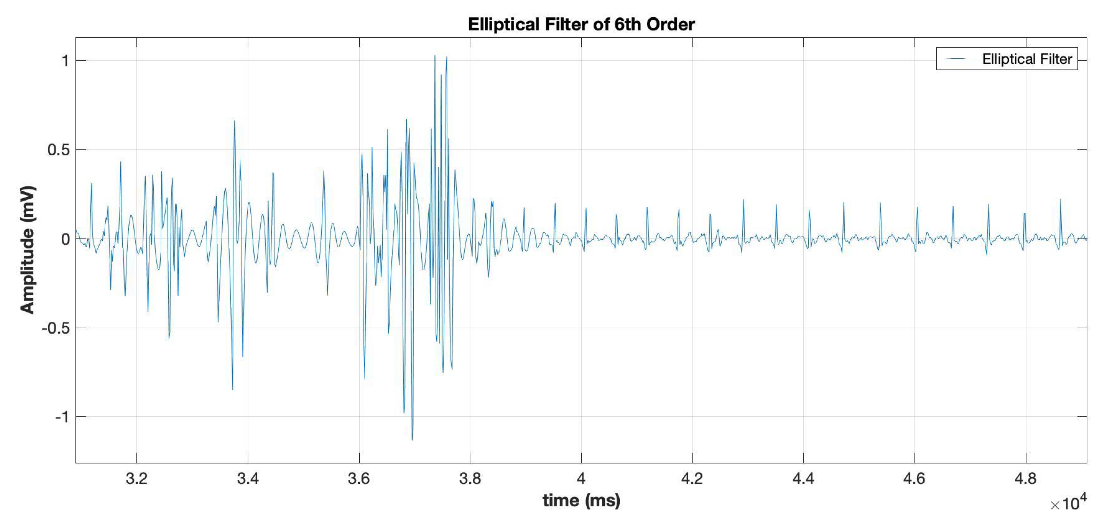
The frequency spectrum (the graph between frequency and amplitude of the signal) of the signals was initially analyzed to detect noises. A harmonic of about 1.5 Hz was observed in the spectrum. These harmonics are most probably due to the power line interface (PLI) because the frequency multipliers (harmonics) are PLI characteristics. A baseline wander is also seen in some of the readings (Figure 3a,b).
The goal of filtering is to remove maximum noise while still preserving the characteristics and properties of the signal. With a wide range of filtering techniques available choosing the right filter presents a challenge in itself. The next step after the identification of a type of artifact in our signal is to choose an appropriate filter. ECG signal filtering is a vital step for ECG signal processing and analysis.
Several different techniques exist in literature to remove noise from ECG signals. References [45,46,47] used wavelet transform to remove baseline drift and reducing overall noise. Similarly, [47] uses an ECG simulation to compare different techniques to remove baseline wander in order to preserve changes in ECG wave and found wavelet-based baseline cancellation the best method. However, it also recommended the Butterworth high-pass filter because of its computationally fast nature.

5.2.1. IIR Versus FIR

The classification of transfer functions in time domain based on the length of its impulse response sequence leads to transfer functions known as infinite impulse response and finite impulse response. The infinite impulse response or IIR filters have an impulse response that does not become exactly zero after a certain point, but continues indefinitely. Whereas in contrast, with the finite impulse response (FIR) the impulse response is finite in length [48].
One chooses between FIR and IIR filters depending majorly on the relative advantages of the two filter types. Since a challenge in our experimental set up is a lot of subject movement and implementation of ECG de-noising in combination with a smart mobile device (hence a limited resource environment), a careful balance between efficiency and accuracy has to be found. In [49] comparison between windows based FIR and IIR Butter-worth filter was observed and IIR filter was shown to outperform FIR by acquiring a better computational efficiency with a minimal signal distortion. Similarly, in [50], the best trade-off between spectral density and average power was shown by IIR filter (Chebyshev Type II) as compared to its counterpart FIR filters. IIR filters have less computational complexity and hence require less computation power as compared to FIR filters. The memory requirement is also increased in the case of FIR filters hence IIR filters can be the better choice for removing baseline noises [50]. Wavelet analysis is also used in recent works to denoise ECG data. Reference [45] used discrete wavelet transformation (DWT) to correct baseline wander and reduce noise. They estimated the baseline wander through coarse approximation in DWT and proposed recommendations for the selection of wavelets and the maximum depth for decomposition level.

5.2.2. Elliptical Filter

To acquire a given level of performance, a much higher filter order is required in case of FIR as compared to IIR. This causes a greater delay in these filters for an equal performing IIR filter.
First of all, the minimum order of an elliptic filter which is required to meet a set of filter design specifications was determined and then same order was used to filter all the signals.
Elliptic filter was better fitted to the data but it not only removed the PLI in the signal, but baseline wander was considerably improved as well.

5.3. Implementation Protocol: Hardware and Software

The following section gives a detailed account of the implementation process for phase I. Now we have filtered ECG signals from the previous step and we want to use a pre-trained CNN, AlexNet, to differentiate between falling and resting ECG signals.
After filtration, each signal of 90 s duration was individually examined and divided in 3 readings in such a way that precisely one fall or at least more than 70% of the fall laid in each reading. This was done to increase the dataset and homogenize the data at one–time duration i.e., 30 s. At this point the collected signals for Daily Activities were considered a part of the class No-Fall.
Two models were trained on different hardware resources for phase I. One with a GeForce RTX 2080 Ti GPU with computing capability of 7.5 and another with a PC containing Intel(R) Core(TM) i5-7260U 2.20 GHz CPU.

5.4. Time-Frequency Representations

The scale-frequency representations were created using SCALOGRAM_CREATION(Ts). Each ECG signal had to be of the same length in order to compute a continuous wavelet transform (CWT) filter bank for all of them. It had to be done carefully so that no valuable signal, specifically fall signals, are lost.
In the next step, CWT filterbank for one of the signals was computed and using those coefficients, time-frequency representations called scalograms for rest of the data were created. Morse wavelet was used to calculate the wavelet transform. The scalograms were saved for later processing. Each representation was of 227 × 227 × 3 sized RGB image as it is the expected input format for AlexNet.
Figure 4a–c provide a comparison between falling and non-falling scalograms. It can be seen that scalogram with a fall in them have some areas with high energy concentration in them in yellow color. On the contrary, the energy seems to be distributed evenly in non-fall ECG scalogram representing the cardiac cycle. Then those images were divided randomly into training and validation data with 80% training images and 20% testing images.

5.5. Phases of Our Implementation

The whole study was conducted (see Table 2) in two major phases as explained in following section. In phase I, the ECG signals obtained by our own experimental set up were used to create wavelet transforms and scalograms. The model trained in this phase had two classification classes: No-Fall which included all readings which did not have fall, and Fall which had signals with fall in them. Eventually, we fine tuned and retrained AlexNet to obtain a trained CNN model which gave 98.02% validation accuracy. (Phase II is described in Section 5.6 below).

5.5.1. Training The Network: Phase I

In phase I, a very small number of daily activities along with resting in no-fall scenarios were included. The daily activities included fast walking, sitting up from laying, sudden standing from sitting, picking up something from the ground while standing and stumbling while fast walking. The daily activities were performed in a domestic setting. Each activity duration ranged between 20 to 30 s.
These were also processed in the same manner as the previous readings in the earlier iteration. Two training sessions were done in this iteration, one with Intel i5, 1.3 GHz and another with the GPU.

5.5.2. Preparing and Training the Model

In transfer learning, a large dataset is used to train a primary network and the features learned from the training are either re-purposed or transferred to an another designated network to be trained on a specific dataset and task. It is usually very difficult to acquire a dataset of sufficient size to train an entire CNN from scratch so practically in most scenarios a CNN is pre-trained on a very large dataset and then used either as initialization or as a feature extractor for the required task. This process is called transfer training. This process works if the features are more generic and suitable to both primary and target tasks and not specific to the basic task [51].
In our case, since the dataset was small, the chances of over-fitting are a concern for using transfer learning. A pre-trained network, AlexNet, was used to train the model and the deeper layers of the network were fine-tuned. Fine-tuning is the closest solution to our problem because universal features like edges or curves are captured by a pre-trained network which is trained on a large and diverse dataset like ImageNet [52]. According to [53], despite the differences between natural images and medical images, the CNNs trained on the well annotated ImageNet can still be transferred to make medical image recognition tasks more effective. It is conjectured that by fine–tuning the transfer learning strategy yields the best results for performance in medical imaging [53] and our experiments confirm this conjecture.

5.5.3. Tuning The AlexNet

As part of any transfer-learning approach the AlexNet had to be fine-tuned to our dataset. The last three layers of AlexNet are configured for 1000 categories and since we have two classification classes, we fine-tuned these layers according to our classification problem. Layer 23 was set to be a fully connected layer of size equal to the number of our classification classes, 2. Layer 24 applies the Softmax and does not need to change. Layer 25 holds the name of the loss function used for training the network and the class labels [54]. Thus, layer 25 was set to be the classification output layer.
The solver algorithm used is “Stochastic Gradient Descent with Momentum” (SGDM). The initial learning rate used for training was set to 1 × 10 4 . The maximum number of epochs were 5 and the size of mini-batch to be used at each epoch was 15. The training was carried out in both a CPU and a GPU.

5.5.4. Activation’s of Different Layers in CNN

Each layer of the CNN produces a specific response to the original image called activations which can be viewed to investigate and learn further how the network learns and what features are adapted by the model to recognize falls. The activations of different layers can be viewed and one can discover which features are learned by the network by comparing areas of activation with the original image. This can also help if we want to manually extract the features by looking at different layers and the features they highlighted.
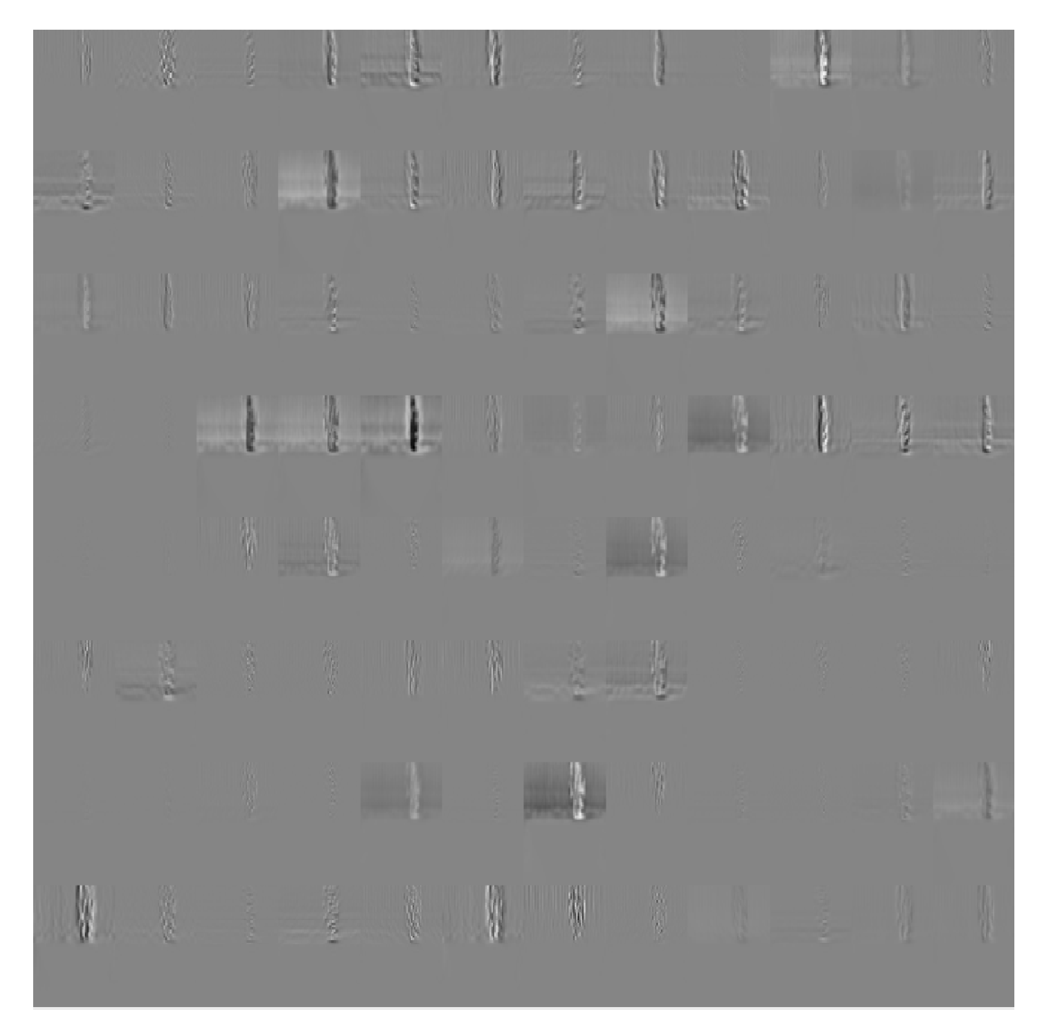
In Figure 5, several tiles can be seen on the grid. Each one is the output of a channel in convolution layer 1 (conv1). Strong positive activation is represented by white pixels and similarly strong negative activations are shown by black pixels. A grey pixel represents moderate activation. The position of the pixels in the activation of a channel corresponds to the same position in the original image [54]. It can be noticed in Figure 5, the network has started to learn about specific fall areas in its activation’s on the first convolution layer. Though it was never explicitly told to learn about this specific fall pattern in scalogram, it has automatically outlined those features in a fall.
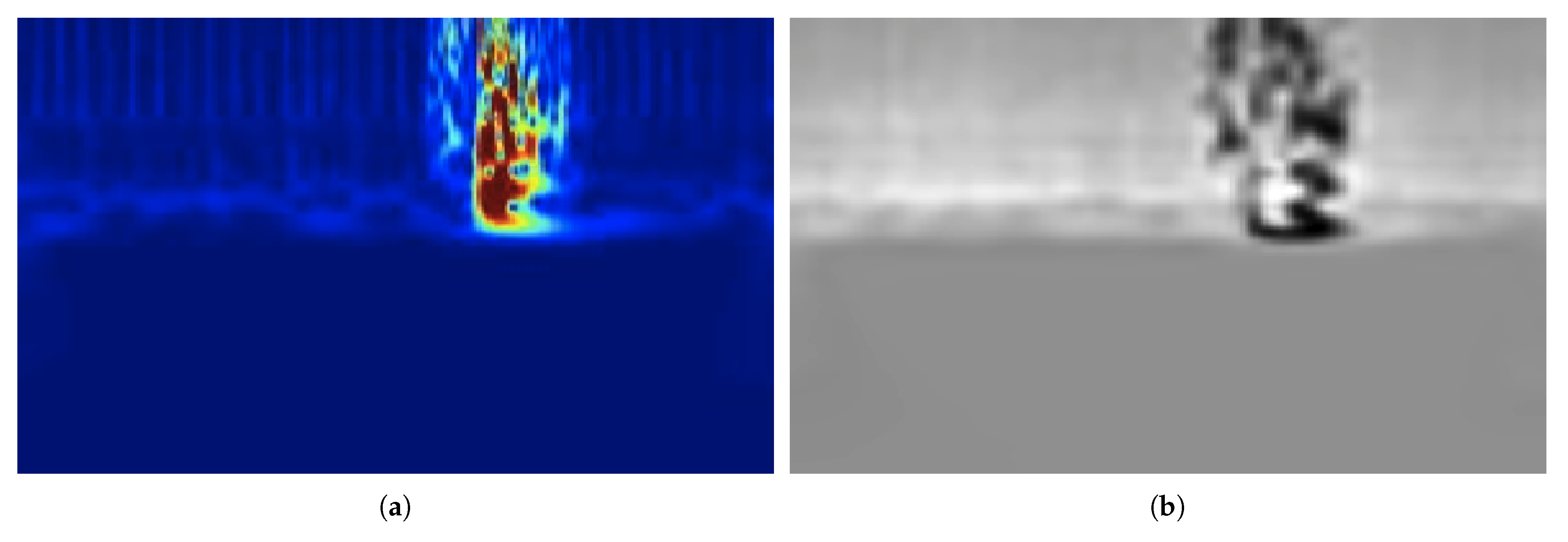
The feature highlighted by the strongest activation in the convolution layer 5 (conv5) in Figure 6 shows that the network correctly highlights the fall feature in a scalogram. Similar patterns can be observed in other scalograms containing falls.
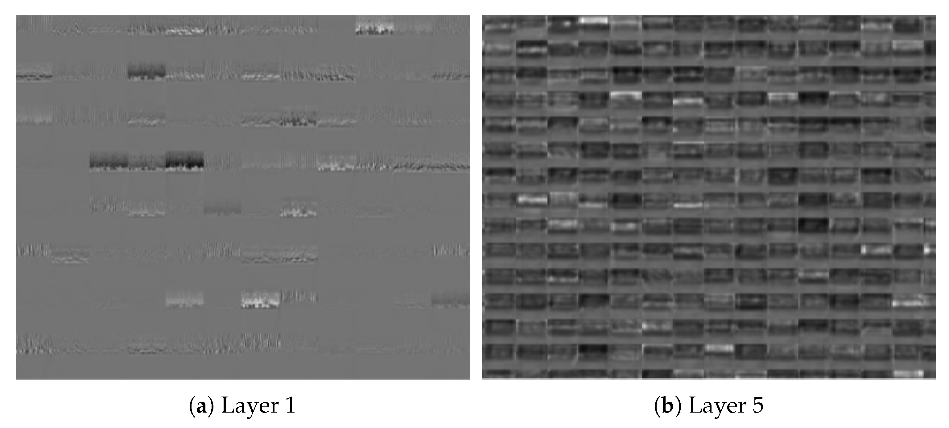
Similarly, by looking at Figure 7, it can be observed that activations of the deeper layer are more specific in features as compared to activations of the earlier layers which are more generic.

5.6. Extension of the Algorithm: Phase II

In the next phase, this study was enhanced by increasing datasets using time series augmentation technique called slicing and adding two different publicly available datasets [28,55]. In this phase another pre-trained CNN called GoogLeNet [56] was trained along with AlexNet [57]. The training for this phase was carried out on a Macbook with 2,6 GHz 6-Core Intel(R) Core(TM) i7. This phase was also concluded with an accuracy of 98.44%.

5.6.1. Data Augmentation and Its Challenges

In order to verify the effectiveness of the proposed algorithm, an additional class was added to our model called Daily Activities. This class encompasses the daily activities which we do in daily life, such as moving around, walking, sitting and jumping. Two publicly available datasets [28,55], were added in the newly defined class. The dataset [28] contains ECG readings from 10 subjects (with mean age of 27, 1 female and 9 males). The signals were recorded performing four body movements—left and right arm up/down, sitting down and standing up and waist twist. Similarly the other database [55], has ECG signals recorded from a healthy 25-year-old male performing different physical activities.
One of the main issues incorporating a new dataset to our existing dataset was the difference in sampling frequencies between the collected data and external data sources. We collected our data at a rate of 62 Hz whereas both external databases have data sampled at a rate of 500 Hz. In order to bring all the data to a common sampling frequency, our collected ECG dataset was interpolated at a rate of 5. Interpolation works better as compared to simple upsampling or resampling. In MATLAB function upsample(), zeroes are inserted between the corresponding values. Similarly in resample(), an anti-aliasing filter is applied after interpolation, which causes a drastic decrease in frequency amplitude. Hence, the function interpolation was used instead of upsample() and resample().
In the previous phase, the dataset collected by us was limited and convolutional networks tend to over-fit with limited datasets. Hence, it was vital to augment the available data. Very few techniques exist in the field of time series augmentation specifically for deep neural networks [58]. We have used the method called windows slicing for augmenting the ECG signals as described in [59].
For a time series T, T = { T 1 , , T n } , window slicing is described as slicing the T into small snippets such that each snippet S i : j = { t i , t i + 1 , t j } , where 1 i j n .
The slicing operation is described as follows [59]:
S l i c i n g ( T , s ) = { S 1 : s , S 2 : s + 1 , , S n s + 1 : n }
In our case, the length of each slice was 4000 and the TS was sliced at every 1000th interval. Thus, each time series signal of length n gave us { n 4000 / 1000 } signals. All the time series generated by Slicing(T,s) will have the same label as that of T.

5.6.2. Tuning the GoogLeNet

Along with AlexNet, GoogLeNet was trained in phase II to obtain a comparative analysis of transfer learning. GoogLeNet, like AlexNet, is also a pre-trained convolutional neural networks. Introduced in [56], GoogLeNet was a winner of ILSVRC 2014 classification and detection challenges. Since the pre-trained models are already trained on a large image set, fine tuning them would provide a simpler and efficient solution to the issue of data shortage for deep learning problem specifically in medical domain. Now our model would have three classification classes, namely, Fall, Resting and Daily Activities.
GoogLeNet has 144 layers as compared to 25 layers in AlexNet. It expects an input image of size 224 × 224 × 3. GoogLeNet introduced a novel feature called inception. It replaces the fully connected architecture with sparse architecture inside the network. The size of convolution filter is fixed in earlier CNN models like AlexNet, and VGGNet. However, now multiple convolution filters of varying size and a maxpooling is done altogether for the previous layer, and the result is stacked together again at output. This not only leads to extraction of different features but it is also computationally efficient [56].
Fine tuning GoogLeNet requires redefining some layers of the network. First of all, final drop out layer is replaced with a probability of 0.6 instead of 0.5. The last two layers, ‘loss3-classifier’ and ‘output’ are replaced with layers which are in accordance with our classification scheme. The layer ‘loss3-classifier’ is replaced to classify three classes instead of 1000. Finally, the last layer ‘classification’ is replaced with a new layer with out any classification labels. The output classes would be set accordingly during the training time.

5.6.3. Transfer Learning to the Rescue: GoogLeNet and AlexNet

Even after applying data augmentation and adding an external database, our database reached a total of 1273 (see Table 2), which would not suffice to train any CNN from scratch for the risk of over-fitting. This kind of situation is far too common in the medical field due to strict data protection and privacy laws and unavailability of domain specific data. Transfer learning can be the answer to various questions in this regard. A pre-trained model is already trained on a huge dataset; in the case of most CNNs, IMAGENET [60]. They have their inner layers already generalized enough to extract the relevant features from a new domain. Hence, training on a new domain can be achieved even on a small or mid-sized dataset. We just have to re-train outer most layers to readjust their weights. Hence, it is also resource friendly.
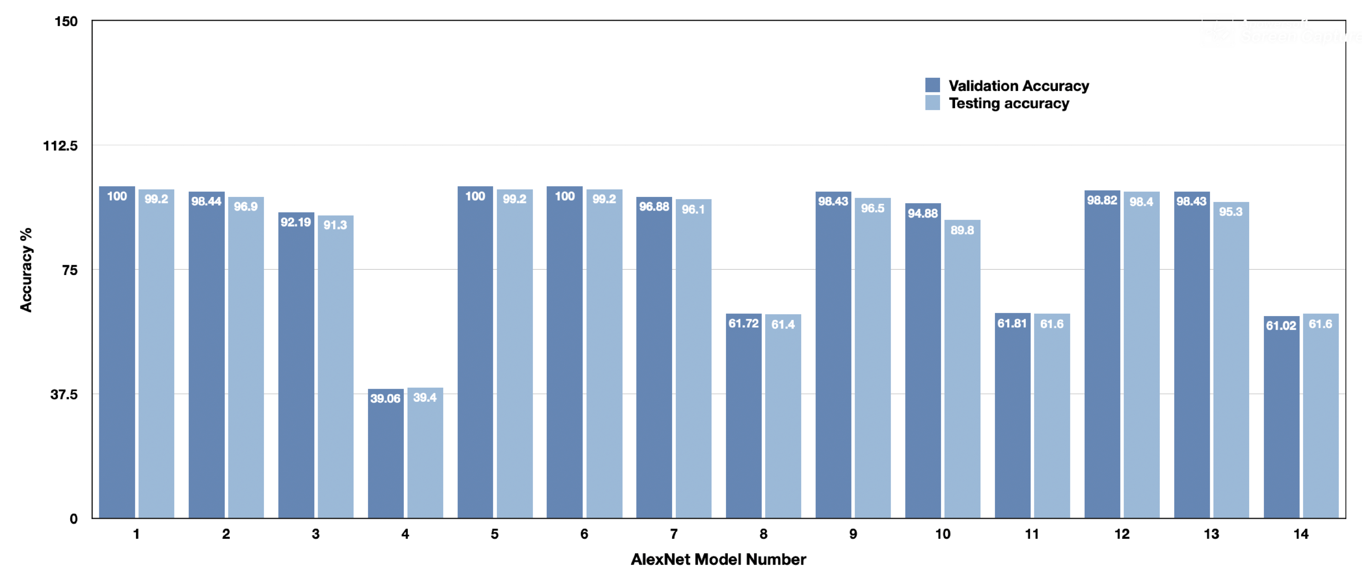
A number of models, both AlexNet and GoogLeNet, were trained. The different parameters, such as initial learning rate (ILR), training algorithm, percentage of validation-training-testing data were varied in order to verify the generalization of the model and proposed algorithm. Training algorithms called Stochastic gradient descent with momentum (SGDM) and Root Mean Square Propagation (RMSprop) were used with similar configurations to compare the outcome. SGDM is a stochastic approximation method initially proposed in [61] with a momentum added to it [62]. RMSprop was initially proposed and explained by Geoff Hinton in an online course [63] and is an unpublished optimization algorithm. The summary of the trained models and the results are shown in Table 3 and Table 4. Out of many trained models, Model 2 from Table 4 (marked as blue) was selected as the most suitable trained model. Model 5 and 6 were not chosen despite of a perfect 100% validation accuracy because they might be over-fitted. Similarly, Model 12 was not chosen because the percentage of validation data is greater in Model 2 (0.8-0.1-0.1) than in Model 12 (0.6-0.2-0.2). A confusion matrix for testing data of Model 2 is shown in Table 5. The last row and column in the confusion matrix indicate the total number of correct predictions expressed in percentage. For example, if we look at the first column, 55 instances of Daily Activities are correctly predicted as Daily Activities and 5 of them were incorrectly predicted as Fall by the model. This amounts to a total correct prediction percentage of 91.7% for daily activities. Similarly, out of a data of 255 instances, 246 were correctly predicted which amounts for a total accuracy of 96.5%.
A graphical summary of the training result is shown in Figure 8.

5.6.4. K-Fold Verification

A k-fold verification was applied on model number 2 from Table 4, as a measure to estimate the generalization of the model. Keeping the size of dataset in mind, k was set to 3. The dataset was divided in three equal parts. At each split, one set was used as the training data and the trained model was tested on both validation and testing data to obtain validation and testing accuracy respectively. An average validation accuracy of 97.69% and a testing average accuracy of 97.37% was achieved. An overview of the process is depicted in Table 6—the blue colour in the table indicates the part of data used as training data, whereas black indicates the segment used as testing data.

6. Analysis of Results

In this section analysis of different results is done to obtain a better understanding of the process.

6.1. Analysis of Fall Vs No-Fall ECG Signals

Figure 9a shows a FallECG with three falls in it. It can be observed that the amplitude has increased significantly in three areas. This can be contributed to either noise due to hit during the fall or due to an actual increase in cardiac activity. The increase lasts for about 1.6 s and then immediately goes back to normal. This time duration coincides with the time taken for the body to touch the ground. This increase in amplitude is of special interest to us. When zoomed in, as shown in Figure 9b the increase goes to an amplitude of 1 mV maximum and is followed by normal cardiac activity as we can see the normal QRS complex after the fall peaks. The other smaller peaks in heart rate in other areas are due to the movements of the subjects from the ground back to the table. The same pattern is repeated with small differences in all other recorded falls.
Figure 10 is a closer look at another fall from the ECG signal in Figure 9a. This fall is also of the same duration (1.6 s) as of in Figure 9b.
Figure 11 gives a side-by-side view of the time domain signals and the corresponding frequency domain of the signals for all three classes of the model. A distinct frequency spectrum can be seen in Figure 11 for Fall, Resting and Daily Activities. The fall is visible in time domain and is also characterized by a spike in frequency domain. The daily activities ECG graph shows considerable noise even after filtration. This is due to the constant movement of the subjects resulting in baseline wander.

6.2. Analysis of Scalograms

The scalogram is obtained by plotting the absolute value of CWT of a signal as a function of time and frequency. They are helpful in visualization of varying events in a signal. Scaling and shifting are used on a prototype wavelet to highlight the transient changes in the signal. We used ‘Morse’ wavelet as a prototype wavelet because its form is very similar to the ECG shape. The fall scalograms shown in Figure 4 have distinct localized high energy areas whereas the resting scalograms have high energy distributed all over the diagram. Now the comparison between Daily Activities scalogram with fall scalogram is interesting. The scalogram of daily activity is shown in Figure 4a. The high energy is distributed almost uniformly all over the representation. If we compare the Daily Activities to the fall scalogram (Figure 4c), it can be clearly seen that noise or high energy due to movements can be seen throughout the daily activities in contrast to a localized high energy area in fall scalogram. Additionally, the magnitude of the energy is different for Resting and Daily Activities scalograms.

7. Discussion of the Research Question

It is evident from the extension of phase I, that even after adding an additional class, the model is trained well and is generalized enough after varying the parameters. With the addition of an external database, the model has learned well the classification task.
This answers our basic research question, which was, “can a fall be detected using an ECG signal?” It is shown that not only can we detect fall in ECG signals but we were able to do it with an accuracy of greater than 90%. As for changing the parameters, it is noticeable from Table 3 and Table 4, how initial learning rate plays the most significant role in determining the validation accuracy. Varying the parameters like the algorithm and the dataset ratio does not make significant change in the validation or testing accuracy. It can be also seen from the tables that by keeping all other parameters constant, the choice of neural network does not make any significant difference in the results.
Hence, a roll over fall has some characteristics imprinted in electrocardiogram signals, which are detectable in time-scale domain (scalograms). That is why the models have learned to distinguish a fall activity from a no fall activity A visible difference with respect to energy distribution can be seen in different activities. These characteristics are distinguishable from an ECG of a resting person or a person performing daily activities. More investigation still needs to be done in the frequency spectrum of ECG signal to learn more about the pattern specific to the fall and other activities.
Our algorithm has obtained an accuracy of more than 97%, greater than that achieved in [20]. Although in [20], different movements were classified using traditional deep learning techniques and fall was not among those activities.
However, our experimental setup is not free of limitations. The focus of this paper has been on determining proof of concept in laboratory and by no means this is a deployment ready prototype. The initial experimental population is considerably small. That was compensated in the second phase by adding two different external datasets. Both datasets not only increased the instances numerically but also brought variation with respect to number of subjects, age and type of noise and signals. Both datasets had obtained signals using different devices. All these factors strengthens our proof of concept. We are also bounded by the obvious limitations of the controlled experimental set up. For example, the subjects have to wear the safety gadgets (helmet, knee caps, etc.) in order to comply with the safety regulations. This might cause an onset of anxiety and nervousness in volunteers, which in turn may effect the heart rate signals. However, these circumstances are unavoidable and we have to take them as experimental conditions.

8. Conclusions and Future Work

It is shown clearly that ECG signals can be utilized alone for not only distinguishing different activities but also fall from no-fall activities by using a combination of wavelet transform and transfer learning. The transfer learning models learned as efficiently and accurately as any other convolutional neural networks trained from scratch. In future, we plan to further analyze the transfer learning approach for time series classification by directly training the ECG signals using long short-term memory (LSTM) networks. Additionally, a detailed frequency spectrum analysis of signals can be performed to extract the features specifically present in different activities. Further experiments are planned to be carried out to include different kind of falls, activities and circumstances. As discussed in the previous section, because of the limited dataset initially acquired, we plan to carry out our experiments on a larger and more diverse (in terms of age and gender) group of people together with a hugely increased set of data to improve this study. Another extension we would like to do is to test our proposed algorithm with state of the art pre-trained networks, such as EfficientNet [64].

Author Contributions

Conceptualization L.L.B., F.S.B., J.S. and M.F.W.; methodology F.S.B., J.S. and M.F.W.; validation F.S.B.; formal analysis F.S.B., J.S. and M.F.W.; resources F.S.B.; data curation L.L.B., and F.S.B.; writing—original draft preparation F.S.B.; writing—review and editing J.S., I.M.-B., D.G.-U. and M.F.W.; visualization F.S.B.; supervision J.S., I.M.-B., D.G.-U. and M.F.W. All authors have read and agreed to the published version of the manuscript.

Funding

This research was funded by the research support program of Fb2, Frankfurt University of Applied Sciences. The research of D.G.-U. has been supported in part by the Spanish MICINN under grants PGC2018-096504-B-C33 and RTI2018-100754-B-I00, the European Union under the 2014-2020 ERDF Operational Programme and the Department of Economy, Knowledge, Business and University of the Regional Government of Andalusia (project FEDER-UCA18-108393). The research of I.M.-B. has been supported in part by the European Commission (ERDF), the Spanish Ministry of Science, Innovation and Universities [RTI2018-093608-BC33].

Institutional Review Board Statement

Our study was conducted with healthy volunteers. Each participant gave written consent to allow measurement data and images to be anonymized and used for publications. A risk assessment was established with assistance from the medical doctor, safety officer and occupational safety specialist of the university, which includes safety precautions to minimize all possible injury risks. These precautions had to be strictly respected, and all participants were instructed and encouraged to follow our instructions before starting the tests to prevent injury. Our study was conducted in accordance with the ethical principles of the Declaration of Helsinki.

Informed Consent Statement

Informed consent was obtained from all subjects involved in the study.

Data Availability Statement

All data is available at https://doi.org/10.21227/x6w8-h979.

Acknowledgments

We thank the volunteers who participated in the fall detection experiments for their time and effort. Their valuable input has lead to beneficial results which were critical to this study. We are thankful to Lorena Gutiérrez-Madroñal from the Department of Computer Science and Engineering, University of Cádiz for her software and assistance in the initial filtration of the raw ECG sensor files. We would also like to thank Sameen Arshad for her insight during the validation of ECG sensor readings and for her medical advice on ECG analysis.

Conflicts of Interest

The authors declare no conflict of interest.

Sample Availability

Data and scripts are available at https://doi.org/10.21227/x6w8-h979.

Abbreviations

The following abbreviations are used in this manuscript:
ADCAnalog to Digital Conversion
BLEBluetooth Low Energy
CNNConvolutional Neural Network
CPUCentral Processing Unit
CVComputer Vision
CWTContinuous Wavelet Transform
DADaily Activities
ECGElectrocardiogram
FIRFinite Impulse Response
GPUGraphics Processing Unit
HARHuman Activity Recognition
IIRInfinite Impulse Response
ILRInitial Learning Rate
LSTMLong Short-Term Memory
PLIPower Line Interface
RMSpropRoot Mean Square Propagation
SGDMStochastic Gradient Descent with Momentum

References

  1. World Health Organization. WHO Global Report on Falls Prevention in Older Age; WHO: Geneva, Switzerland, 2007. [Google Scholar]
  2. Allcock, L.M.; O’Shea, D. Diagnostic yield and development of a Neuro cardiovascular investigation unit for older adults in a district hospital. J. Gerontol. Ser. A Biol. Sci. Med Sci. 2000, 55, M458–M462. [Google Scholar] [CrossRef] [PubMed] [Green Version]
  3. Tinetti, M.E. Factors Associated with Serious Injury During Falls by Ambulatory Nursing Home Residents. J. Am. Geriatr. Soc. 1987, 35, 644–648. [Google Scholar] [CrossRef] [PubMed]
  4. Wild, D.; Nayak, U.S.; Isaacs, B. How dangerous are falls in old people at home? Br. Med. J. 1981, 282, 266–268. [Google Scholar] [CrossRef] [PubMed] [Green Version]
  5. Wang, Z.; Ramamoorthy, V.; Gal, U.; Guez, A. Possible Life Saver: A Review on Human Fall Detection Technology. Robotics 2020, 9, 55. [Google Scholar] [CrossRef]
  6. Genoud, D.; Cuendet, V.; Torrent, J. Soft Fall Detection Using Machine Learning in Wearable Devices. In Proceedings of the 2016 IEEE 30th International Conference on Advanced Information Networking and Applications (AINA), Crans-Montana, Switzerland, 23–25 March 2016; pp. 501–505. [Google Scholar] [CrossRef]
  7. Lu, N.; Wu, Y.; Feng, L.; Song, J. Deep Learning for Fall Detection: Three-Dimensional CNN Combined with LSTM on Video Kinematic Data. IEEE J. Biomed. Health Inform. 2019, 23, 314–323. [Google Scholar] [CrossRef]
  8. Lundervold, A.S.; Lundervold, A. An overview of deep learning in medical imaging focusing on MRI. Z. Med. Phys. 2019, 29, 102–127. [Google Scholar] [CrossRef]
  9. Tan, C.; Sun, F.; Kong, T.; Zhang, W.; Yang, C.; Liu, C. A Survey on Deep Transfer Learning. In Artificial Neural Networks and Machine Learning— ICANN 2018; Kůrková, V., Manolopoulos, Y., Hammer, B., Iliadis, L., Maglogiannis, I., Eds.; Springer International Publishing: Berlin/Heidelberg, Germany, 2018; pp. 270–279. [Google Scholar]
  10. Pan, S.J.; Yang, Q. A Survey on Transfer Learning. IEEE Trans. Knowl. Data Eng. 2010, 22, 1345–1359. [Google Scholar] [CrossRef]
  11. Xu, T.; Zhou, Y.; Zhu, J. New Advances and Challenges of Fall Detection Systems: A Survey. Appl. Sci. 2018, 8, 418. [Google Scholar] [CrossRef] [Green Version]
  12. Igual, R.; Medrano, C.; Plaza, I. Challenges, issues and trends in fall detection systems. Biomed. Eng. Online 2013, 12, 66. [Google Scholar] [CrossRef] [Green Version]
  13. Vallabh, P.; Malekian, R. Fall detection monitoring systems: A comprehensive review. J. Ambient. Intell. Humaniz. Comput. 2018, 9, 1809–1833. [Google Scholar] [CrossRef]
  14. Wang, Y.; Jiang, X.; Cao, R.; Wang, X. Robust Indoor Human Activity Recognition Using Wireless Signals. Sensors 2015, 15, 17195–17208. [Google Scholar] [CrossRef] [PubMed] [Green Version]
  15. Damodaran, N.; Schäfer, J. Device Free Human Activity Recognition using WiFi Channel State Information. In Proceedings of the 2019 IEEE SmartWorld, Ubiquitous Intelligence Computing, Advanced Trusted Computing, Scalable Computing Communications, Cloud Big Data Computing, Internet of People and Smart City Innovation (SmartWorld/SCALCOM/UIC/ATC/CBDCom /IOP/SCI), Leicester, UK, 19–23 August 2019; pp. 1069–1074. [Google Scholar] [CrossRef]
  16. Damodaran, N.; Haruni, E.; Kokhkharova, M.; Schäfer, J. Device free human activity and fall recognition using WiFi channel state information (CSI). CCF Trans. Pervasive Comput. Interact. 2020, 2, 1–17. [Google Scholar] [CrossRef] [Green Version]
  17. Jia, R.; Liu, B. Human daily activity recognition by fusing accelerometer and multi-lead ECG data. In Proceedings of the 2013 IEEE International Conference on Signal Processing, Communication and Computing (ICSPCC 2013), KunMing, China, 5–8 August 2013; pp. 1–4. [Google Scholar] [CrossRef]
  18. Castro, D.; Coral, W.; Rodriguez, C.; Cabra, J.; Colorado, J. Wearable-Based Human Activity Recognition Using an IoT Approach. J. Sens. Actuator Netw. 2017, 6, 28. [Google Scholar] [CrossRef] [Green Version]
  19. Addison, P.S. Wavelet transforms and the ECG: A review. Physiol. Meas. 2005, 26, R155–R199. [Google Scholar] [CrossRef] [Green Version]
  20. Kher, D.R.; Pawar, T.; Thakar, D. Impact Analysis of Body Movements on Wearable Ambulatory Electrocardiogram; OMICS International: Hyderabad, India, 2015. [Google Scholar] [CrossRef]
  21. Turan, A.; Barshan, Ö.; Barshan, B. Detecting Falls with Wearable Sensors Using Machine Learning Technique. Sensors 2014, 14, 10691–10708. [Google Scholar]
  22. Md Shahiduzzaman. Fall detection by Acceleromeer and Heart rate variability Measurement. Glob. J. Comput. Sci. Technol. G Interdiscip. 2015, 15. Available online: https://computerresearch.org/index.php/computer/article/view/1328 (accessed on 29 January 2021).
  23. MathWorks. Classify Time Series Using Wavelet Analysis and Deep Learning. Available online: https://de.mathworks.com/help/wavelet/examples/signal-classification-with-wavelet-analysis-and-convolutional-neural-networks.html (accessed on 20 August 2018).
  24. Hoang, H.V.; Tran, M. DeepSense-Inception: Gait Identification from Inertial Sensors with Inception-like Architecture and Recurrent Network. In Proceedings of the 2017 13th International Conference on Computational Intelligence and Security (CIS), Hong Kong, China, 15–18 December 2017; pp. 594–598. [Google Scholar] [CrossRef]
  25. Melillo, P.; Castaldo, R.; Sannino, G.; Orrico, A.; de Pietro, G.; Pecchia, L. Wearable technology and ECG processing for fall risk assessment, prevention and detection. In Proceedings of the 2015 37th Annual International Conference of the IEEE Engineering in Medicine and Biology Society (EMBC), Milan, Italy, 25–29 August 2015; pp. 7740–7743. [Google Scholar] [CrossRef]
  26. Butt, F.S. Fall Detection Using Machine Learning Techniques on ECG Signals. Master’s Thesis, Frankfurt University of Applied Sciences, Frankfurt am Main, Germany, 2019. [Google Scholar]
  27. Kim, Y.G.; Shin, D.; Park, M.Y.; Lee, S.; Jeon, M.S.; Yoon, D.; Park, R.W. ECG-ViEW II, a freely accessible electrocardiogram database. PLoS ONE 2017, 12, e0176222. [Google Scholar] [CrossRef]
  28. Goldberger, A.L.; Amaral, L.A.N.; Glass, L.; Hausdorff, J.M.; Ivanov, P.C.; Mark, R.G.; Mietus, J.E.; Moody, G.B.; Peng, C.K.; Stanley, H.E. PhysioBank, PhysioToolkit, and PhysioNet: Components of a new research resource for complex physiologic signals. Circulation 2000, 101, e215–e220. [Google Scholar] [CrossRef] [Green Version]
  29. La Blunda, L.; Corral-Plaza, D.; Wagner, M.; Ortiz, G.; Medina-Bulo, I. Distributed real-time based human activity analysis system. In Proceedings of the 16th International Conference on Applied Computing in Cagliari (ITALY), Cagliari, Italy, 7–9 November 2019; Volume 6. [Google Scholar]
  30. La Blunda, L. Fall event Analysis based on sensor fusion. In Proceedings of the Las Jornadas Predoctorales de la Escuela Superior de Ingeniería (JORPRESI), Cádiz, Spain, 2 November 2017. [Google Scholar]
  31. La Blunda, L.; Gutiérrez-Madroñal, L.; Wagner, M.F.; Medina-Bulo, I. A Wearable Fall Detection System Based on Body Area Networks. IEEE Access 2020, 8, 193060–193074. [Google Scholar] [CrossRef]
  32. World Medical Association. World Medical Association Declaration of Helsinki: Ethical principles for medical research involving human subjects. JAMA 2013, 310, 2191–2194. [Google Scholar] [CrossRef] [Green Version]
  33. Dickinson, D.F. The normal ECG in childhood and adolescence. Heart 2005, 91, 1626–1630. [Google Scholar] [CrossRef] [PubMed] [Green Version]
  34. Sucerquia, A.; López, J.; Vargas-Bonilla, J.F. SisFall: A Fall and Movement Dataset. Sensors 2017, 17, 198. [Google Scholar] [CrossRef]
  35. Fleming, J.; Brayne, C. Inability to get up after falling, subsequent time on floor, and summoning help: Prospective cohort study in people over 90. BMJ 2008, 337. [Google Scholar] [CrossRef] [PubMed] [Green Version]
  36. Jing, N. Detecting Human Falls with a 3-Axis Digital Accelerometer. Analog Dialogue 2009, 43, 3. [Google Scholar]
  37. Roggen, D.; Calatroni, A.; Rossi, M.; Holleczek, T.; Förster, K.; Tröster, G.; Lukowicz, P.; Bannach, D.; Pirkl, G.; Ferscha, A.; et al. Collecting complex activity datasets in highly rich networked sensor environments. In Proceedings of the 2010 Seventh International Conference on Networked Sensing Systems (INSS), Kassel, Germany, 15–18 June 2010; pp. 233–240. [Google Scholar] [CrossRef] [Green Version]
  38. Ordóñez, F.J.; Roggen, D. Deep Convolutional and LSTM Recurrent Neural Networks for Multimodal Wearable Activity Recognition. Sensors 2016, 16, 115. [Google Scholar] [CrossRef] [Green Version]
  39. Reiss, A.; Stricker, D. Physical Activity Monitoring Data Set. 2012. Available online: http://archive.ics.uci.edu/ml/datasets/PAMAP2+Physical+Activity+Monitoring (accessed on 2 February 2021).
  40. Zappi, P.; Lombriser, C.; Stiefmeier, T.; Farella, E.; Roggen, D.; Benini, L.; Tröster, G. Activity Recognition from On-Body Sensors: Accuracy-Power Trade-Off by Dynamic Sensor Selection. In European Conference on Wireless Sensor Networks; Springer: Berlin/Heidelberg, Germany, 2008; pp. 17–33. [Google Scholar]
  41. Guan, Y.; Plötz, T. Ensembles of Deep LSTM Learners for Activity Recognition Using Wearables. In Proceedings of the ACM on Interactive, Mobile, Wearable and Ubiquitous Technologies; ACM: New York, NY, USA, 2017; Volume 1. [Google Scholar] [CrossRef] [Green Version]
  42. Analog to Digital Conversion. Available online: https://learn.sparkfun.com/tutorials/analog-to-digital-conversion/all (accessed on 2 December 2018).
  43. Manivel, K.; Ravindran, R.S. Noise Removal for Baseline wander and power line in Electrocardiograph Signals. Int. J. Adv. Res. Electr. Electron. Instrum. Eng. 2015, 4, 1114–1122. [Google Scholar]
  44. Das, N.; Chakraborty, M. Performance Analysis of FIR and IIR filters for ECG Signal De-noising based on SNR. In Proceedings of the 2017 Third International Conference on Research in Computational Intelligence and Communication Networks (ICRCICN), Kolkata, India, 3–5 November 2017. [Google Scholar]
  45. Zhang, D. Wavelet Approach for ECG Baseline Wander Correction and Noise Reduction. In Proceedings of the 2005 IEEE Engineering in Medicine and Biology 27th Annual Conference, Shanghai, China, 1–4 September 2005; pp. 1105–1108. [Google Scholar]
  46. Ara, I.; Hossain, M.N.; Mahbub, S.Y. Baseline drift removal and de-noising of the ECG signal using Wavelet Transform. Int. J. Comput. Appl. 2014, 95, 15–17. [Google Scholar] [CrossRef]
  47. Lenis, G.; Pilia, N.; Loewe, A.; Schulze, W.H.W.; Dössel, O. Comparison of Baseline Wander Removal Techniques considering the preservation of ST changes in the Ischemic ECG: A simulation Study. Comput. Math. Methods Med. 2017, 2017, 9295029. [Google Scholar] [CrossRef]
  48. Sanjit, K.M. Digital Signal Processing; McGraw-Hill: New York, NY, USA, 1998. [Google Scholar]
  49. Milchevski, A.; Guse, M. Performance Evaluation of FIR and IIR Filtering of ECG Signals. In International Conference on ICT Innovations; Springer: Berlin/Heidelberg, Germany, 2016; pp. 103–112. [Google Scholar]
  50. Rani, S.; Kaur, A.; Ubhi, J.S. Comparative study of FIR and IIR filters for the removal of Baseline noises from ECG signal. Int. J. Comput. Sci. Inf. Technol. 2011, 2, 1105–1108. [Google Scholar]
  51. Yosinski, J.; Clune, J.; Bengio, Y.; Lipson, H. How transferable are features in deep neural networks? In Advances in Neural Information Processing Systems 27; Ghahramani, Z., Welling, M., Cortes, C., Lawrence, N.D., Weinberger, K.Q., Eds.; Curran Associates, Inc.: Red Hook, NY, USA, 2014; pp. 3320–3328. [Google Scholar]
  52. ImageNet. Available online: http://www.image-net.org/ (accessed on 7 December 2018).
  53. Shin, H.; Roth, H.R.; Gao, M.; Lu, L.; Xu, Z.; Nogues, I.; Yao, J.; Mollura, D.J.; Summers, R.M. Deep Convolutional Neural Networks for Computer-Aided Detection: CNN Architectures, Dataset Characteristics and Transfer Learning. IEEE Trans. Med Imaging 2016, 35, 1285–1298. [Google Scholar] [CrossRef] [Green Version]
  54. Visualize Activations of a Convolutional Neural Network. Available online: https://de.mathworks.com/help/deeplearning/examples/visualize-activations-of-a-convolutional-neural-network.html (accessed on 10 December 2018).
  55. Kher, R. Wearable Ambulatory Electrocardiogram (ECG) and EEG Dataset. IEEE Dataport. 2020. [Google Scholar] [CrossRef]
  56. Szegedy, C.; Liu, W.; Jia, Y.; Sermanet, P.; Reed, S.; Anguelov, D.; Erhan, D.; Vanhoucke, V.; Rabinovich, A. Going Deeper with Convolutions. In Proceedings of the Computer Vision and Pattern Recognition (CVPR), Boston, MA, USA, 7–12 June 2015. [Google Scholar]
  57. Krizhevsky, A.; Sutskever, I.; Hinton, G.E. ImageNet Classification with Deep Convolutional Neural Networks. In Advances in Neural Information Processing Systems; Pereira, F., Burges, C.J.C., Bottou, L., Weinberger, K.Q., Eds.; Curran Associates, Inc.: Red Hook, NY, USA, 2012; Volume 25, pp. 1097–1105. [Google Scholar]
  58. Iwana, B.K.; Uchida, S. An Empirical Survey of Data Augmentation for Time Series Classification with Neural Networks. arXiv 2020, arXiv:2007.15951. [Google Scholar]
  59. Cui, Z.; Chen, W.; Chen, Y. Multi-Scale Convolutional Neural Networks for Time Series Classification. arXiv 2016, arXiv:1603.06995. [Google Scholar]
  60. Deng, J.; Dong, W.; Socher, R.; Li, L.J.; Li, K.; Fei-Fei, L. Imagenet: A large-scale hierarchical image database. In Proceedings of the 2009 IEEE Conference on Computer Vision and Pattern Recognition, Miami, FL, USA, 20–25 June 2009; pp. 248–255. [Google Scholar]
  61. Robbins, H.; Monro, S. A stochastic approximation method. Ann. Math. Stat. 1951, 22, 400–407. [Google Scholar] [CrossRef]
  62. Qian, N. On the momentum term in gradient descent learning algorithms. Neural Netw. 1999, 12, 145–151. [Google Scholar] [CrossRef]
  63. Geoffrey Hinton, N.S.; Swersky, K. Neural Networks for Machine Learning Online Course. Available online: https://www.classcentral.com/course/neuralnets-398 (accessed on 2 February 2021).
  64. Tan, M.; Le, Q.V. EfficientNet: Rethinking Model Scaling for Convolutional Neural Networks. arXiv 2020, arXiv:1905.11946. [Google Scholar]
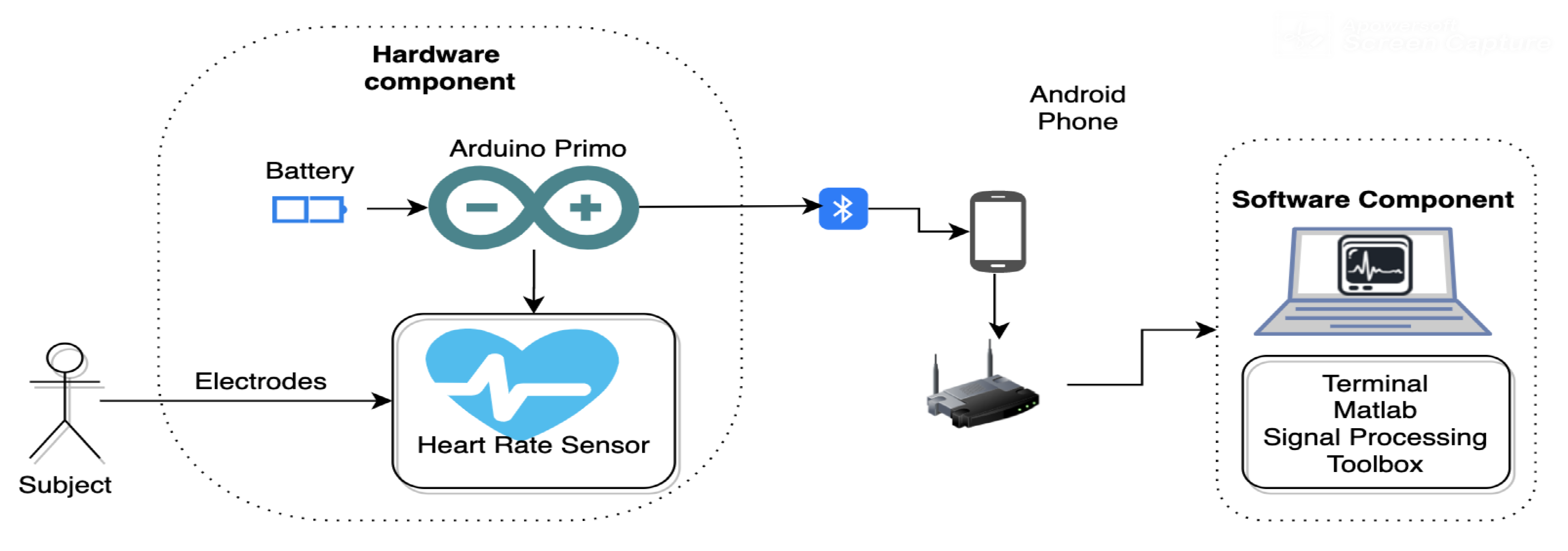
Figure 1. The system architecture diagram for a data acquisition system—hardware and software components [30].
Information 12 00063 g001
Figure 2. The rollover fall process.
Information 12 00063 g002
Figure 3. Examples of baseline wander.
Information 12 00063 g003
Figure 4. Scalograms with different classes of ECG signal in them.
Information 12 00063 g004
Figure 5. Scalogram of the FallECG: activations in The conv1 Layer For the fall scalogram.
Information 12 00063 g005
Figure 6. Scalogram of the Fall ECG and its corresponding activation. (a) Scalogram with a distinct Fall; (b) strongest activation of the image in layer 5 (conv5).
Information 12 00063 g006
Figure 7. Scalogram Of Resting ECG: activations of earlier and deeper layers.
Information 12 00063 g007
Figure 8. A graphical summary of the training results for the AlexNet model.
Information 12 00063 g008
Figure 9. Falls in ECG signals in the time domain. (a) An ECG signal with three falls; (b) the fall pattern immediately followed by normal heart activity.
Information 12 00063 g009
Figure 10. A closer look at the fall activity in an ECG Signal.
Information 12 00063 g010
Figure 11. A comparison of different ECG time domain signals with their corresponding frequency spectrum. (a) Time domain ECG signal for Daily Activities. (b) Frequency domain ECG signal for Daily Activities. (c) Time domain ECG signal for Fall. (d) Frequency domain ECG signal for Fall. (e) Time domain ECG signal for Resting. (f) Time domain ECG signal for Resting.
Information 12 00063 g011
Table 1. A summary of the collected data.
No.Participant IdGenderAgeExperiment DurationTotal Fall ReadingsTotal Resting ReadingsTotal DA ReadingsDuration of each FallDuration of each Resting Duration of each DA
1Sub1M35120 min513590 s90 s30 s
2Sub2M5250 min310090 s90 s0
3Sub3F3050 min60090 s0 s0
4Sub5F32120 min2536590 s30 s30 s
5Sub6M4045 min80090 s0 s0
6Sub7M1845 min100090 s0 s0
Table 2. Total number of samples used for training in both iterations.
Reading TypeTotal Count (Phase I)Total Count (Phase II)
Fall153500
Resting104474
Daily Activities-296
Total2571270
Table 3. Summary of GoogLeNet fine-tuned and retrained for fall detection using ECG signals with different parameters.
No.AlgorithmTrain.-Val.-Testing RatioILRVal. AccuracyTesting Accuracy
1SGDM0.8-0.1-0.1 10 4 98.44%95.3%
2SGDM0.8-0.1-0.1 10 5 95.31%93.7%
3SGDM0.8-0.1-0.1 10 6 85.94%86.6%
4RMSprop0.8-0.1-0.1 10 2 39.06%39.4%
5RMSprop0.8-0.1-0-1 10 4 98.44%98.4%
6RMSprop0.8-0.1-0-1 10 5 100%97.6%
7RMSprop0.8-0.1-0-1 10 6 96.09%92.1%
8RMSprop0.8-0.1-0-1 10 9 37.50%37.0%
Table 4. Summary of AlexNet fine-tuned and retrained for fall detection using ECG signals with different parameters.
No.AlgorithmTrain-Val.-Test RatioILRVal. AccuracyTesting Accuracy
1SGDM0.8-0.1-0.1 10 4 100%99.2%
2SGDM0.8-0.1-0.1 10 5 98.44%96.9%
3SGDM0.8-0.1-0.1 10 6 92.19%91.3%
4RMSprop0.8-0.1-0.1 10 2 39.06%39.4%
5RMSprop0.8-0.1-0-1 10 4 100%99.2%
6RMSprop0.8-0.1-0-1 10 5 100%99.2%
7RMSprop0.8-0.1-0-1 10 6 96.88%96.1%
8RMSprop0.8-0.1-0-1 10 9 61.72%61.4%
9SGDM0.6-0.2-0.2 10 5 98.43%96.5%
10SGDM0.6-0.2-0.2 10 6 94.88%89.8%
11SGDM0.6-0.2-0.1 10 9 61.81%61.6%
12RMSprop0.6-0.2-0-2 10 5 98.82%98.4%
13RMSprop0.6-0.2-0-2 10 6 98.43%95.3%
14RMSprop0.6-0.2-0-2 10 9 61.02%61.6%
Table 5. Confusion matrix for the selected trained model.
Actual
Daily ActivitiesFallRestingTotal (in Percentage)
PredictedDaily Activities551098.2%
Fall596095.0%
Resting039596.9%
Total (in percentage)91.7%96.0%100%96.5%
Table 6. An overview of k-fold verification.
Fold 1Fold 2Fold 3Val AccuracyTest Accuracy
Split 1Fold 1Fold 2Fold 397.65%98.2%
Split 2Fold 1Fold 2Fold 398.04%97.4%
Split 3Fold 1Fold 2Fold 397.39%96.5%
Training data, Testing data Average Accuracy97.69%97.36 %
Publisher’s Note: MDPI stays neutral with regard to jurisdictional claims in published maps and institutional affiliations.