Learnable Leaky ReLU (LeLeLU): An Alternative Accuracy-Optimized Activation Function

Abstract

In neural networks, a vital component in the learning and inference process is the activation function. There are many different approaches, but only nonlinear activation functions allow such networks to compute non-trivial problems by using only a small number of nodes, and such activation functions are called nonlinearities. With the emergence of deep learning, the need for competent activation functions that can enable or expedite learning in deeper layers has emerged. In this paper, we propose a novel activation function, combining many features of successful activation functions, achieving 2.53% higher accuracy than the industry standard ReLU in a variety of test cases.

1. Introduction

Activation functions originated from the attempt to generalize a linear discriminant function in order to address nonlinear classification problems in pattern recognition. Thus, an activation function is a nonlinear, monotonic function that transforms a linear boundary function to a non-linear one. The same principle was used in perceptrons in order to allow the perceptron to classify the inputs. The most straightforward activation function is the identity function (y = x), along with the binary activation function in Equation (1) that resembles an activation/classification switch.

$$y=1 if x>0 or y=0 if x\le 0$$

(1)

This is the first nonlinearity used in perceptrons and multilayer perceptrons and made its way to more complex neural networks later on. Despite its simplicity, the discontinuity at x = 0, which rendered the calculation of the corresponding derivative rather difficult, encouraged the search for new monotonic and continuous activation functions. The first continuous, nonlinear activation function that was used was the sigmoid, also called the logistic or the soft-step activation function, and is described by Equation (2).

$$\sigma \left(x\right)=\frac{1}{1+e^{-x}}$$

(2)

This allowed the computation of nonlinear problems by using a low number of neurons. The sigmoid was used in the hidden layers of common neural networks and enabled the training and inference of these systems for years. A similar function can arise from the sigmoid function through a linear transformation of the input and the output is the Hyperbolic tangent (Tanh) presented in Equation (3).

$$\tanh \left(x\right)=\frac{e^x-e^{-x}}{e^x+e^{-x}}$$

(3)

Again, this was widely used in neural networks for years, and it was generally accepted that the Tanh function favored faster training convergence, compared to the sigmoid function. However, the computation of these activation functions is rather expensive, since it entails look-up table solutions; thus, they are non-optimal choices for neural networks. The emergence of deeper architectures and deep learning, in general, has also highlighted another deficit of the two traditional activation functions. Their bounded output restricted the dissipation of derivatives in back-propagation when the network was deep. In other words, deeper layers received almost zero updates to their weights; that is, they were able to learn during the training process. This phenomenon is also known as the vanishing gradient problem.

The difficulty in computational calculation and deep learning is partially solved with the introduction of the rectified linear unit (ReLU) [1] in Equation (4).

$$y=\max \left\{0,x\right\}=x | x>0$$

(4)

The ReLU achieves great performance, while being computationally efficient. Since it poses no restriction on positive inputs, gradients have more chances to reach deeper layers in back-propagation, thus enabling learning in deeper layers. In addition, the computation of the gradient in backpropagation learning is reduced to a multiplication with a constant, which is far more computationally efficient. Thus, a whole new era in learning and inference with neural networks has emerged, dominating the last decade.

One drawback of the ReLU is that it does not activate for non-positive inputs, causing the deactivation of several neurons during training, which can be viewed again as a vanishing gradient problem for negative values. The non-activation for non-positive numbers is solved with the introduction of the Leaky rectified linear unit (Leaky ReLU) [2], which activates slightly for negative values, as expressed in Equation (5).

$$y=\{\begin{array}{cc}0.01x & if x<0\\ x& if x\ge 0\end{array}$$

(5)

One can encounter a number of other variations of ReLU in the literature. One basic variation of the ReLU is the Parametric Rectified Linear Unit (PReLU) [3], which has a learnable parameter, α, controlling the leakage of the negative values, presented in Equation (6). In other words, PReLU is a Leaky ReLU; however, the slope of the curve for negative values of x is learnt through adaptation instead of being set at a predetermined value.

$$y=\{\begin{array}{cc}\alpha x & if x<0\\ x& if x\ge 0\end{array}$$

(6)

Moving away from the family of ReLU, we see that there is the Gaussian Error Linear Unit (GELU) [4] in Equation (7). This activation function is non-convex and non-monotonic and features curvature everywhere in the input space. The authors in Reference [4] claim that GELU can offer a regularization effect on the trained network, since the output is determined on both the input and the stochastic properties of the input. Thus, neurons can be masked off the network, based on the statistical properties of x, which resembles the batch normalization [5] and the Drop-out [6] mechanisms.

$$y=\frac{1 }{2 }x(1+\mathrm{erf}(\frac{x}{\sqrt{2}}))=x\Phi \left(x\right)$$

(7)

Another nonlinear activation function is the Softplus [7,8], as described by Equation (8). The Softplus function features smooth derivatives and less computational complexity, as compared to the GELU; however, it is still more complex compared to the ReLU family.

$$y=\ln \left(1+e^x\right)$$

(8)

The exponential linear unit (ELU) [9] in Equation (9) is another smooth, continuous and differentiable function that tackles the vanishing gradient problem for negative values through an exponential function. This function saturates for great negative values; however, the degree of saturation is controlled by the learnable parameter, α.

$$y=\alpha \left(e^x-1\right) if x\le 0 or y=x if x>0$$

(9)

The scaled exponential linear unit (SELU) [10] is another version of the ELU with controllable parameters that induce self-normalizing properties.

$$y=\lambda \alpha \left(e^x-1\right) if x\le 0 or y=\lambda x if x>0$$

(10)

where the values of α = 1.6733 and λ = 1.0507.

These last activation functions act similar to the ReLU family, providing slightly higher accuracy in complex problems, while having higher computational cost due to the exponential/logarithmic part in the computation and the more complicated implied derivatives at back-propagation.

In Reference [11], Courbariauxet et al. introduced a stricter version of the original sigmoid function, coined “hard sigmoid”, which is given by the formula:

$$y=\max (0,\min (1,\frac{x+1}{2}))$$

(11)

The proposed function was less computationally expensive as compared to the original sigmoid and yielded better results in its experiments [11].

Another derivative from the original sigmoid function is the Swish activation function, which was introduced in Reference [12] and is described by the following formula:

$$y=\mathrm{swish}\left(x\right)=x \mathrm{sigmoid}\left(\beta x\right)=\frac{x}{1+e^{-\beta x}}$$

(12)

where β can be a fixed or a trainable parameter. Swish can be regarded as a smooth function that serves as an intermediate between a linear function and a ReLU.

Finally, the Mish activation function [13] is a self-regularized non-monotonic activation function that was inspired by the Softplus function and Swish and is described by the following:

$$y=x \tanh \left(\ln \left(1+e^x\right)\right)$$

(13)

There is no trainable/adjustable parameter here, nonetheless, it seems to outperform Swish and other functions in a study [13]. The computational complexity of estimating the function is noteworthy in this case.

More complicated activation functions have also recently been proposed. In Reference [14], Maguolo et al. propose the Mexican ReLU, which is described by the following equation:

$$y=PReLU\left(x\right)+{{\displaystyle \sum }}_{j=1}^{k-1}{c}_j{\phi }_{aj,\lambda j }\left(x\right)$$

(14)

where ${\phi }_{a,\lambda }\left(x\right)=\max \left(\lambda -\left|x-a\right|, 0\right)$ is a Mexican-hat-type function, and a and λ are learnable parameters. In Reference [15], the concept of reproducing activation functions is introduced, where a different activation function is applied to each neuron. The applied activation function is a weighted combination of a set of known activation functions with learnable parameters and weights for each neuron. In Reference [16], Zhou et al. define the activation function as a trainable piecewise linear unit with five learnable parameters for each neuron. In Reference [17], Shridhar et al. introduce the concept of a stochastic activation function, where y = μ(x) + σε, where ε is drawn randomly from a Gaussian pdf with N(0,1), σ is a trainable or static parameter and μ(x) can be a static or learnable function, usually initialized by the ReLU. In Reference [18], Bingham and Miikkulainen propose a genetic algorithm to create customized activation functions from a family of well-known activation functions. The evolution begins with a parent activation function that evolves through four evolutionary operations (insert, remove, change and regenerate). Each function that is generated is parameterized, and a fitness score is estimated. The functions that yield the best fitness scores are added to the population of activation functions to be used in the NN.

The objective of the paper is to propose a novel activation function that (a) expands the ReLU family by adding support to the negative values; (b) the degree of saturation for the negative values is controlled by a learnable parameter, α; (c) this parameter α simultaneously controls a learning boost for positive values; (d) in the case of α → 0, the learning at these nodes ceases, leading to a regularization of the network, similar to Drop-out, which eliminates the need of such techniques; (e) the accuracy performance gain of the proposed activation function over ReLU increases with the information complexity of the dataset (i.e., the difficulty of the problem); and it (f) remains a simple function with a single learnable/adaptive parameter and a simple update rule, in contrast to far more complicated adaptive activation functions.

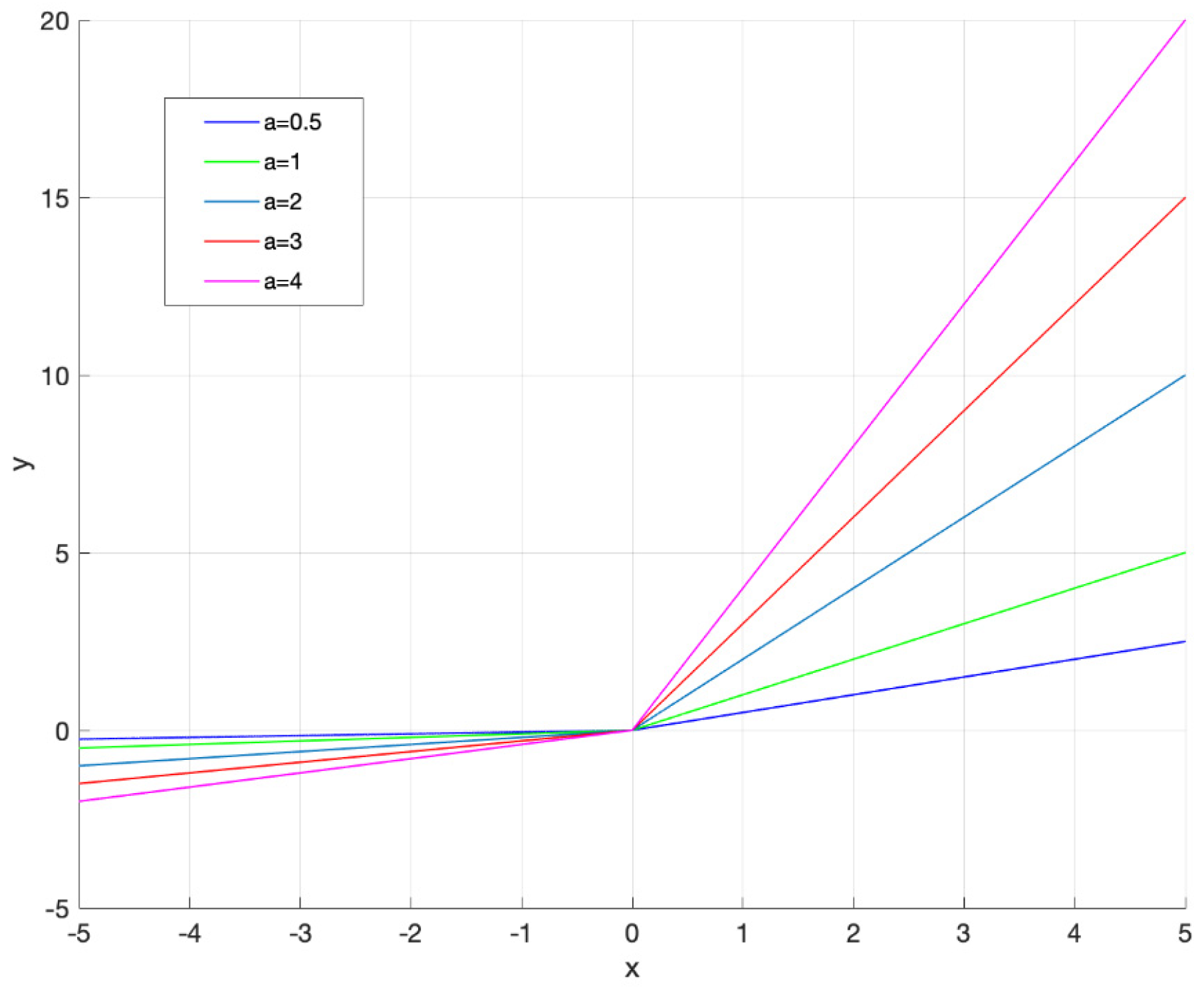
2. The Proposed Activation Function

In this paper, we propose a novel activation function combining the best qualities of the ReLU family, while having low computational complexity and more adaptivity to the actual data. The equation that describes the Leaky Learnable ReLU (LeLeLU) is as follows:

$$y=\alpha \max \left(x,0\right)+0.1\alpha \min \left(0,x\right)$$

(15)

$$y=\{\begin{array}{cc}0.1\alpha x & if x<0\\ \alpha x& if x\ge 0\end{array}$$

(16)

where α is a learnable parameter that controls the slope of the activation function for negative inputs, but what is different here is that it simultaneously controls the slope of the activation function for all positive inputs. There is a constant multiplier, 0.1, that reduces the slope for negative input values in a similar manner to the Leaky ReLU, which seems to work well in our experiments. LeLeLU is depicted in Figure 1 for various values of α.

The derivative of LeLeLU can simply be calculated by the following:

$$\frac{dy}{dx}=\{\begin{array}{cc}0.1\alpha & if x<0\\ 0& if x=0\\ \alpha & if x>0\end{array}$$

(17)

The update formulations of the parameter α can be derived by using the chain rule. The gradient of α for one layer for each neuron, i, can be given by the following:

$$\frac{\partial L}{\partial {\alpha }_i}={\displaystyle \sum }_{y_i}\frac{\partial L}{\partial f\left(y_i\right)}\frac{\partial f\left(y_i\right)}{\partial {\alpha }_i}$$

(18)

where L(•) denotes the neural network’s loss function, and y_i denote the output of the i-th neuron.

In order to reduce the computational cost in demanding situations, one can choose to keep the parameter α the same for a number of neurons, i.e., for a layer. For the layer-shared variant, the gradient of α is as follows:

$$\frac{\partial L}{\partial \alpha }={\displaystyle \sum }_i{\displaystyle \sum }_{y_i}\frac{\partial L}{\partial f\left(y_i\right)}\frac{\partial f\left(y_i\right)}{\partial \alpha }$$

(19)

where the summation Σ_i sums over all neurons of the layer. The complexity overhead of α, the learnable parameter, is negligible for both forward and backward propagation, while gradient descent with the momentum method was used during training.

$${\alpha }_i^{+}\leftarrow \mu {\alpha }_i-\eta \frac{\partial L}{\partial {\alpha }_i}$$

(20)

where η is the learning rate, and μ denotes momentum.

The parameter α is learnable per filter during training, and during testing, we observed a correlation between dataset complexity, depth-wise position of respective filter in the neural network topology and training phase.

It is obvious in Figure 1 that, for α = 1, our proposed activation function turns into the leaky ReLU activation function. The strong point of the proposed activation function is that the learnable parameter influences both the negative and the positive values. This implies that the adaptation of α can accelerate training in certain parts of the network during certain epochs of the training procedure, when α gets values that are larger than 1. In contrast, when α gets lower than 1 values, learning slows down for certain parts of the network.

In the special case that α gets values close to zero, not only learning is halted for these neurons, but their output is close to zero, which implies that these neurons are severed from the network. Hence, by de-activating several neurons, the network is automatically regularized during training in a similar manner to the popular Drop-out technique [6]. The difference is that, by using the proposed activation function, network regularization is performed by the adaptation of the activation function and network training, whereas a Drop-out is a mechanism that works as an extra step during network training. The adaptation of the parameter α is investigated in more detail in the next section.

3. Parameter Adaptation and Network Regularization

In this section, we investigate the role and behavior of parameter α during training. As a testbed, we used the Fashion MNIST dataset and the corresponding network architecture in Figure 2. The programming environment was MATLAB 2020a on a Haswell i7 4770 s, 16 GB DDR3 RAM, NVidia GTX 970 4 GB PC, running Windows 10. The code for implementing LeLeLU can be found here (https://github.com/ManiatopoulosAA/LeLeLU, accessed on 10 October 2021).

In the proposed network architecture, we included the use of Batch Normalization [5], which is a form of network regularization that keeps the mean and variance of neurons’ output normalized. The use of Drop-out is often complementary to Batch Normalization; therefore, we can see in the literature that they can be used in parallel. Since the proposed activation function is similar to PReLU, we would like to compare the performance of the proposed activation function with PReLU on the previously described testbed. In addition, since the proposed activation function is performing regularization in the same manner as Drop-out, we would like to compare its performance with a combination of PReLU, using Drop-out on each layer.

The results are very conclusive. The architecture using PReLU only yields classification accuracy of 0.82, with notably slower convergence. The architecture using PReLU and Drop-out yields a classification accuracy of 0.829, whereas the proposed activation function with batch normalization but without Drop-out achieves an accuracy of 0.912. Thus, at first, LeLeLU performed better than PReLU itself. At the same time, LeLeLU is performing better than PReLU with a regularizer (Drop-out). This implies that the adaptation of LeLeLU is regularizing the network itself and even works better than Drop-out by 8.8%. There is an extra computational cost for the adaptation of parameter α. Based on the previous testbed, the runtime of the proposed scheme is marginally longer by 2.56%, compared to the PReLU+Drop-out combination. We reckon that this might be due to the fact that Drop-out completely removes and does not process some neurons from the network, whereas, in our case, the network continues to process these neurons, even in the case that α→ 0 in their LeLeLU.

In Figure 3, we visualized the adaptation of parameter α for a random neuron/filter as it changes for every epoch. It is obvious that there is an active Drop-out-like behavior at least twice for every neuron during the training process, while there are instances where the parameter α is near 1, accelerating the learning of the neuron in question.

4. Results

In this section, we perform a more thorough comparison between the various activation functions for various different datasets.

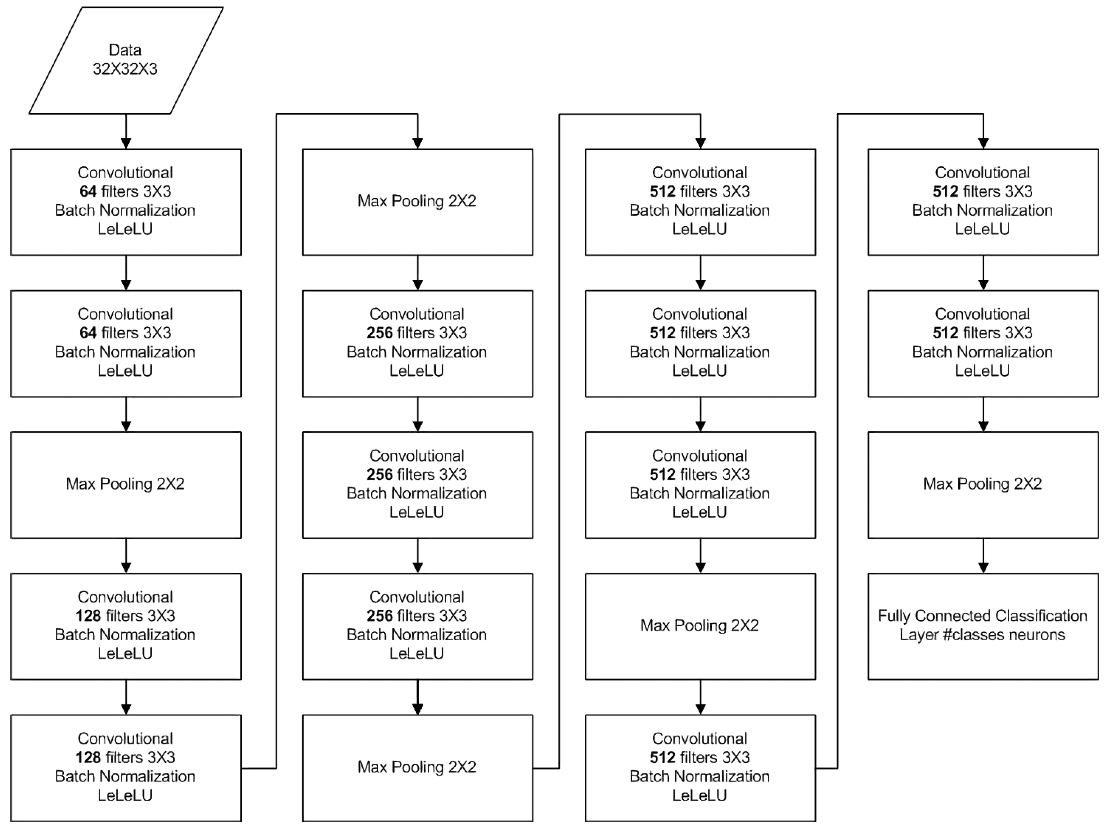
4.1. Datasets and Network Topologies

The topology of all networks used to compare the four activation functions is displayed in Figure 3.

More specifically, MNIST and Fashion MNIST run on a three-hidden-layer convolutional neural network with 16, 32 and 48 5 × 5 filters, while the last layer was a 10-neuron classification layer. The Sign MNIST runs on a five-hidden-layer convolutional neural network with 16, 32 and 48 5 × 5 filters, while the last two hidden layers have 64 and 96 3 × 3 filters, respectively. The last layer is a 24-neuron fully connected classification layer. Lastly, the CIFAR-10 classification dataset runs on a five-hidden-layer convolutional neural network with 32, 36 and 48 5 × 5 filters, while the last two hidden layers have 64 and 96 3 × 3 filters respectively, with the last layer being a 10 neuron classification layer.

The MNIST topology was trained for 15 epochs, the Fashion MNIST for 20 epochs, the Sign Language dataset for 20 and the CIFAR-10 dataset for 60 epochs. Since the scope of this paper is the comparison of different activation functions, and since the ReLU activation function is the most widely known and used, all results presented were normalized to the accuracy obtained used by the ReLU activation.

All testing was conducted with five-fold validation, and the results presented in the next section are the mean of the three median values. In other words, from the five accuracy results of five-fold validation, the largest and lowest values were dropped, and the three median values were averaged to give a more balanced score that is less prone to outliers. In our experiments, we benchmarked the following activation functions: Tanh, ReLU, PReLU, ELU, SELU, HardSigmoid, Mish, Swish and the proposed LeLeLU. These activation functions were chosen as representative examples of each category of baseline activation functions, as described earlier in the introduction. We preferred to compare with simple activation functions with minimal computational cost or adaptation, such as the proposed one, avoiding those mentioned earlier with great adaptation complexity and many trainable parameters.

4.2. Numerical Results

Here, we evaluate all experiments, using accuracy, i.e., the number of correctly classified examples over the total number of examples in the testing dataset. As stated previously, the overall accuracy is estimated via five-fold validation. Then, we consider the accuracy achieved by ReLU as the baseline result, and we calculate normalized accuracy as the ratio (in percentage) of the new activation function accuracy over the accuracy achieved by ReLU.

In

Table 1. Test accuracy in the MNIST dataset of the activation functions in question, using the corresponding neural network, and accuracy normalized to that attained by ReLU activation function.

Activation Function	Accuracy	Normalized Accuracy
ReLU	0.9875	100%
PReLU	0.9861	99.9%
Tanh	0.9835	99.6%
ELU	0.9879	100%
SELU	0.9878	100.04%
HardSigmoid	0.9756	98.79%
Mish	0.9881	100.06%
Swish	0.9878	100.04%
LeLeLU	0.9897	100.23%

, we can see the accuracy and normalized accuracy on the MNIST dataset, using the nine activation functions. All activation functions perform well, with the LeLeLU giving a small boost of 0.23% over the baseline ReLU. The proposed LeLeLU outperforms current state-of-the-art activation functions, including Swish and Mish. The MNIST dataset contains a well-studied and easy-to-classify dataset, and therefore the improvement is minimal but existent. It should be noted that PReLU slightly underperforms in this experiment, but this is minimal.

In

Table 2. Test accuracy in the Fashion MNIST dataset of the activation functions in question, using the corresponding neural network, and accuracy normalized to that attained by ReLU activation function.

Activation Function	Accuracy	Normalized Accuracy
ReLU	0.8956	100%
PReLU	0.8961	100.06%
Tanh	0.8979	100.2%
ELU	0.9071	101.2%
SELU	0.8959	100.03%
HardSigmoid	0.8704	97.19%
Mish	0.9037	100.9%
Swish	0.9019	100.7%
LeLeLU	0.912	101.8%

, we can see the accuracy and normalized accuracy on the Fashion MNIST dataset, using the nine activation functions. All activation functions perform relatively well. The LeLeLU gives a significant boost of 1.8% over the baseline ReLU, whereas PReLU improves slightly by 0.06%, with the ELU giving the second best improvement of 1.2%. Mish and Swish outperform the traditional ReLU, but they are well below the proposed LeLeLU.

In

Table 3. Test accuracy in the Sign Language dataset of the activation functions in question, using the corresponding neural network, and accuracy normalized to that attained by ReLU activation function.

Activation Function	Accuracy	Normalized Accuracy
ReLU	0.9073	100%
PReLU	0.8815	97.2%
Tanh	0.8522	93.9%
ELU	0.8721	96.1%
SELU	0.8196	93%
HardSigmoid	0.8586	97.4%
Mish	0.8974	101.8%
Swish	0.8947	101.5%
LeLeLU	0.9353	103.2%

, we can see the accuracy and normalized accuracy on the Sign Language dataset, using the nine activation functions. Here, the results are more impressive. All other activation functions clearly underperform, as compared to the baseline ReLU, with the LeLeLU giving the only improved performance with a significant boost of 3.2% over the baseline. Here, again, we witness the superiority of the proposed LeLeLU, compared to Mish and Swish, which are the only ones that offer an improvement to ReLU, but their improvement is less impressive than that of the LeLeLU. This experiment clearly demonstrated the significant ability of LeLeLU to adapt over the dataset and improve both positive and negative values learning, as compared to the stationary ReLU.

In

Table 4. Test accuracy in the CIFAR-10 dataset of the activation functions in question, using the corresponding neural network, and accuracy normalized to that attained by ReLU activation function.

Activation Function	Accuracy	Normalized Accuracy
ReLU	0.6829	100%
PReLU	0.7094	103.5%
Tanh	0.6785	99.3%
ELU	0.7065	103.4%
SELU	0.7103	104%
HardSigmoid	0.6652	97.4%
Mish	0.6938	101.6%
Swish	0.6890	100.9%
LeLeLU	0.7166	104.9%

, we can see the accuracy and normalized accuracy on the CIFAR-10 dataset, using the five activation functions. Here, the LeLeLU is again scoring the best improvement over the baseline, with a significant boost of 4.9%. PReLU and ELU have demonstrated improvement in this example of 3.5% and 3.4% respectively, with the Tanh underperforming, as expected. Mish and Swish offer less significant improvement, whereas, SELU is the second runner-up, offering an improvement of 4%.

Overall, LeLeLU shows a consistent tendency to improve classification accuracy over the baseline ReLU, which is not the case for the other tested activation function. PReLU, which is very close to LeLeLU, shows very unstable performance with cases of serious underperformance. It is evident that the performance of all competing tested activation functions depends on the dataset used. Some might underperform or overperform the original ReLU function. Only the proposed LeLeLU seems to consistently offer an improvement in all tested cases. This clearly demonstrates that the addition of a controllable slope (parameter α) in the positive values area of the activation function has improved classification performance. This parameter also controls the speed of adaptation of positive values and seems to improve performance by either accelerating or slowing down learning, in contrast to the fixed slope for positive values of ReLU and PReLU.

4.3. LeLeLU Performance in Larger Deep Neural Networks

In this section, we evaluate the performance of the proposed LeLeLU in more real-life deep network architectures, such as the VGG-16 and the ResNet-v1-56.

4.3.1. VGG-16 with LeLeLU

The first large neural network in our experimentation is the VGG-16, used to classify Cifar-10 and Cifar-100 datasets. The topology of the network and the results for different activation functions are also presented in Reference [17].

The CIFAR-100 dataset is an expansion of the Cifar-10. It has 100 classes, containing 600 images per class. From those 600 images per class, 500 are considered training images and 100 test images per class. The resolution of the images is also 32 by 32 pixels, the same as with Cifar-10.

The VGG-16 topology used in our work is the same with Reference [17], with two convolutional layers with 64 filters, followed by max pooling; two convolutional layers with 128 filters, followed by max pooling; three convolutional layers with 256 filters, followed by max pooling; and two similar blocks of three convolutional layers with 512 filters each, followed by max pooling, one after the other. The final layer is a classification layer. Figure 4 depicts the VGG-16 topology.

In

Table 5. Test accuracy in the CIFAR-10 dataset of the activation functions in question, using the VGG-16 neural network, and accuracy normalized to that attained by ReLU activation function.

Activation Function	Accuracy	Normalized Accuracy
Sigmoid	0.1	11.46%
Tanh	0.1	11.46%
ReLU	0.8727	100%
Leaky ReLU	0.8649	99.1%
PReLU	0.8635	98.94%
ELU	0.8765	100.44%
SELU	0.8665	99.29%
Swish	0.8655	99.17%
LeLeLU	0.8792	100.74%

and

Table 6. Test accuracy in the CIFAR-100 dataset of the activation functions in question, using the VGG-16 neural network, and accuracy normalized to that attained by ReLU activation function.

Activation Function	Accuracy	Normalized Accuracy
Sigmoid	0.01	1.99%
Tanh	0.01	1.99%
ReLU	0.5294	100%
Leaky ReLU	0.4944	93.39%
PReLU	0.4630	87.46%
ELU	0.5660	106.91%
SELU	0.5152	97.31%
Swish	0.5401	102.02%
LeLeLU	0.5632	106.38%

, we depict the performance of VGG-16 for Cifar10 and Cifar100 for various activation functions. We can easily see that the proposed function LeLeLU offers the best or the second best classification accuracy among the competing activation functions and a clear improvement over the widely used ReLU. More specifically, it offers the best performance for Cifar-10 and the second best for Cifar-100, behind ELU. However, it outperforms the more state-of-the-art Swish function, which is more prominent in the modern deep-learning literature. We preferred again to compare against simple activation functions with minimal computational complexity and adaptation. The ProbAct function that is proposed in Reference [17] yields a maximum of 0.8892 for Cifar10 and 0.5583 for Cifar100 for an element-wise bound trainable parameter σ (comparable to ours). Their score is better than LeLeLU in Cifar10, but far worse in Cifar100; however, it should also be noted that the parameter σ should be bound by another sigmoid function during adaptation (i.e., computational complexity) in order to stabilize the performance, which is far more complicated than our simple unbound adaptation rule.

4.3.2. ResNet-v1-56 with LeLeLU

In Reference [18], there is an extensive comparison of various activation functions, using the ResNet-v1-56 architecture for the classification of the Cifar-100 dataset. Here, we use the same topology and training methods as in Reference [18], along with the published results, to compare our proposed activation function. Again, in our comparison, we prefer baseline activation function with minimal complexity, such as the one proposed in this paper.

Table 7. Test accuracy in the CIFAR-100 dataset of the activation functions in question, using the ResNet-v1-56 neural network, and accuracy normalized to that attained by ReLU activation function.

Activation Function	Accuracy	Normalized Accuracy
Sigmoid	0.3647	52.37%
HardSigmoid	0.3255	46.74%
ReLU	0.6964	100%
Leaky ReLU	0.6978	100.2%
GELU	0.7019	100.79%
PReLU	0.7223	103.72%
ELU	0.6967	100.04%
SELU	0.6852	98.39%
Mish	0.6988	100.34%
Swish	0.6968	100.06%
Softplus	0.6971	100.1%
Softsign	0.5838	83.83%
Tanh	0.6388	91.73%
LeLeLU	0.7283	104.58%

contains the classification accuracy for CIFAR-100, along with the proposed function. The proposed LeLeLU activation function enables the network to better adapt to the complex dataset, having the highest classification accuracy in this test. Again, LeLeLU seems to perform better, as compared to modern counterparts, including Mish and Swish. It is also noteworthy that the complicated activation function produced by the genetic algorithm in Reference [18] for the ResNet-v1-56 architecture does not exceed accuracy of 0.7101.

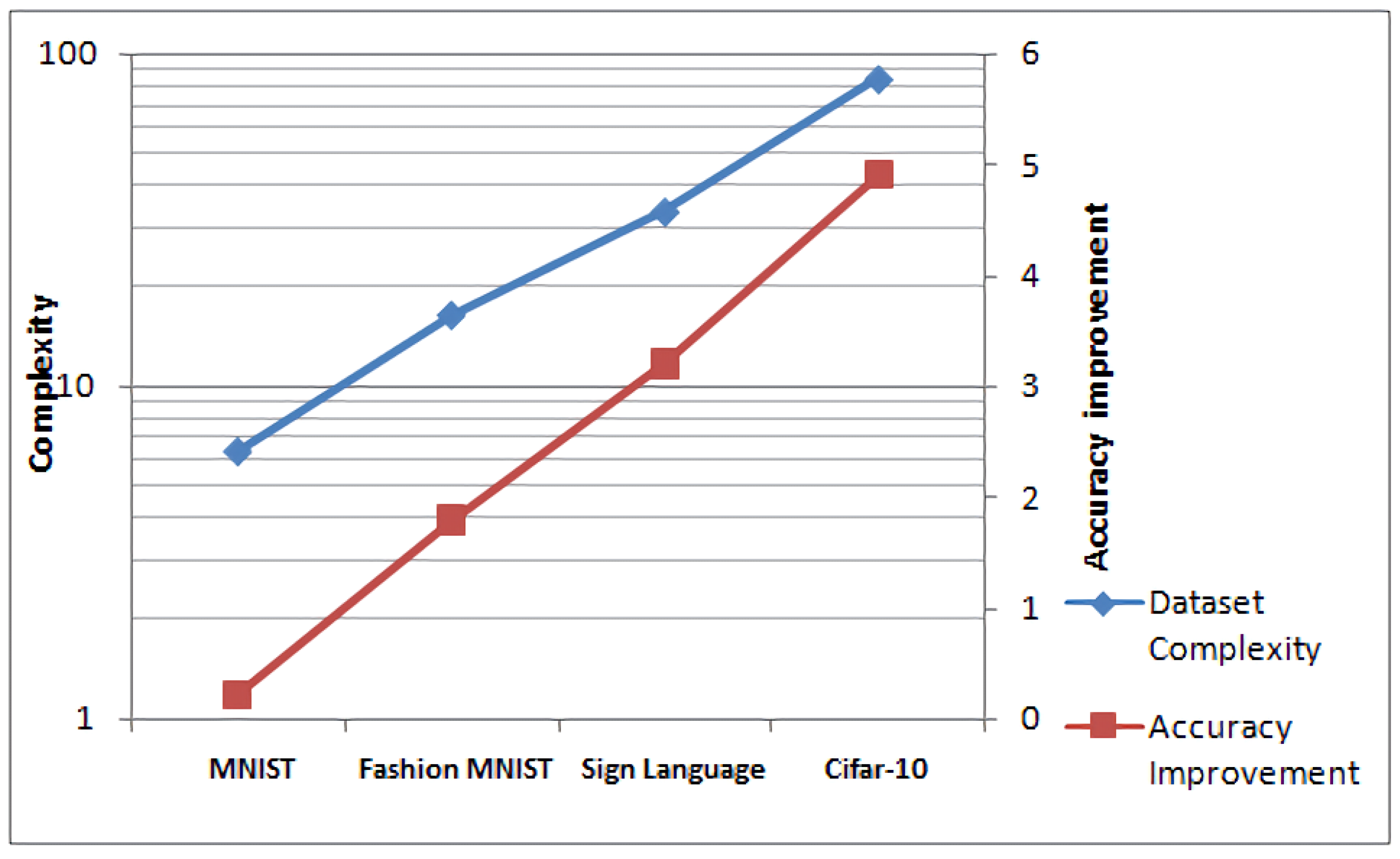
4.4. LeLeLU Performance vs. Dataset Complexity

In this section, we attempt to identify possible correlation between the gain in accuracy, offered by the proposed activation function LeLeLU, and the dataset used in the experiment. We witnessed that in the previous experiments LeLeLU featured an increasing improvement in accuracy. Thus, we attempt to quantify the difference between the four datasets.

One feature of a dataset that we can identify is its complexity. We propose to estimate the complexity of the dataset by using an approximation of the Kolmogorov complexity theorem. Kolmogorov complexity can be defined for any information source. It can be shown [19,20,21] that, for the output of Markov information sources, Kolmogorov complexity is related to the entropy of the information source [22]. More precisely, the Kolmogorov complexity of the output of a Markov information source, normalized by the length of the output, converges most probably to the entropy of the source (since the output’s length can be assumed to go to infinity) [23].

Based on this conclusion, we deduce that it is possible to evaluate the complexity of the dataset by using the product of the mean entropy of each sample and the bits required to represent every category (e.g., 7 for 80 classes). This method is very efficient, even in the case of large datasets. One could also employ only a representative amount of samples from each class and not the full dataset, without generally losing accuracy in the estimation of complexity. The following pseudocode (Algorithm 1) outlines the proposed procedure.

Algorithm 1 Dataset Complexity Estimation

Input: X_train data, number_of_classes Output: Dataset_complexity 1  x_matrix is initialized to the X_train data 2  set number_of_classes to the number of classes of the classification problem 3  set number_of_training_files N to the number of training examples contained in the dataset 4  T ← 0 5  for each data sample in x_matrix 6    calculate the entropy E of the corresponding data sample 7    T ← T + E 8  end for 9  calculate mean entropy (ME): ME ← T/N 10   calculate the bits Q required to represent the number of classes 11   Dataset_complexity = ME × Q

We use the algorithm to estimate the complexity of each dataset used in our experiments. The findings are outlined in

Table 8. Complexity of each dataset of Section 4.2, given the above algorithm and the corresponding LeLeLU accuracy improvement.

Dataset	Complexity	LeLeLU Accuracy Improvement
MNIST	6.41	100.23%
Fashion MNIST	16.466	101.8%
Sign Language	33.584	103.2%
CIFAR-10	83.993	104.9%

. It is clear that the complexity of each dataset correlates highly with the improvement offered by LeLeLU. Figure 5 depicts this finding in a logarithmic plot. We can clearly see that the more complex the dataset is, the bigger the improvement we can attain by using the proposed activation function. It also appears that the improvement is almost analogous to the logarithmic complexity of the dataset (see Figure 5. This implies that the adaptation of the parameter α for positive values helps the overall neural network to adapt faster to the complexity of the dataset, thus giving more improvement compared to the fixed non-adaptive baseline ReLU in more challenging problems.

In this section, we attempt to derive an empirical equation that provides an estimate of the accuracy improvement, offered by the LeLeLU over ReLU, given the complexity of the dataset. The equation that correlates the improvement over ReLU of the proposed function, based on our testing in small arbitrary topologies, is computed by finding the fit function of the two lines of Figure 5 and combining the two equations:

Let C denote the dataset complexity, and x the increasing integer identity of the dataset. The dataset complexity fit function can be estimated by exhaustive parameter search of an exponential function, as follows.

$$\begin{gathered} C=3.159e^{0.789x} \\ ln\left(\frac{C}{3.159}\right)=0.789x \\ x=1.267ln\left(\frac{C}{3.159}\right) \end{gathered}$$

(21)

Let AccImpr denote the accuracy improvement percentage. The accuracy improvement fit function can be estimated by linear fitting, as follows:

$$\begin{gathered} AccImpr=1.54x-2.018 \\ x=\frac{AccImpr+2.018}{1.54} \end{gathered}$$

(22)

By combining Equations (20) and (21), we can conclude the following:

$$\begin{gathered} \frac{AccImpr+2.018}{1.54}=1.267ln\left(\frac{C}{3.159}\right) \\ AccImpr=1.54\ast 1.267\left[ln\left(C\right)-ln\left(3.159\right)\right]-2.018 \\ AccImpr=1.951ln\left(C\right)-1.503-2.018 \end{gathered}$$

Thus, we end up with Equation (23), which yields the accuracy improvement offered by the proposed LeLeLU in terms of the dataset complexity. It is clear that Equation (23) is a monotonic rising function; that is, the more complex the dataset, the more accuracy improvement yielded the proposed LeLeLU.

$$AccImpr=1.951ln\left(C\right)-3.521$$

(23)

To verify the validity of Equation (23), we use the experiment of Cifar-100 with VGG-16, which was not used in the derivation of Equation (23). The Cifar-100 dataset has a complexity of 146.988, and the proposed function achieved an improvement of 6.38% over ReLU, as presented in Table 7. By substituting these figures in Equation (23), we can see that they verify Equation (23) very closely.

$$1.951ln\left(146.988\right)-3.521=6.215\cong 6.38$$

(24)

In essence, Equation (23) provides a very good estimate of the LeLeLU’s performance for any given dataset.

5. Discussion

The activation function is a core component in the neural network topology that affects both the behavior and computational complexity. By combining the best features of the ReLU family, we proposed the Learnable Leaky ReLU (LeLeLU), being linear and, thus, easily computable, while providing the parametric freedom to model the problem effectively. In our experiments, the proposed activation function consistently provided the best accuracy among the tested functions and datasets. It is very interesting that it features an almost analogous increase in accuracy gain to the complexity of the dataset. Thus, LeLeLU assists the network to adapt to the demands of challenging datasets, achieving almost analogous performance gain.

In the future, we will investigate methods to overcome the limitation of having to use batch normalization as a core component when implementing LeLeLU in a network. We will also investigate the effect of using higher-order polynomial versions of the original LeLeLU activation function and/or adding noisy perturbations in a similar manner to ProbAct [17].

References

1. Nair, V.; Hinton, G.E. Rectified Linear Units Improve Restricted Boltzmann Machines. In Proceedings of the 27th International Conference on International Conference on Machine Learning, 2010 ICML’10, Haifa, Israel, 21–24 June 2010; Omnipress: Madison, WI, USA; pp. 807–814, ISBN 9781605589077. [Google Scholar]
2. Maas, A.L.; Hannun, A.Y.; Ng, A.Y. Rectifier nonlinearities improve neural network acoustic models. In Proceedings of the 30th International Conference on Machine Learning, Atlanta, GA, USA, 16–21 June 2013; Volume 30. [Google Scholar]
3. He, K.; Zhang, X.; Ren, S.; Sun, J. Delving Deep into Rectifiers: Surpassing Human-Level Performance on ImageNet Classification. arXiv 2015, arXiv:1502.01852. [Google Scholar]
4. Hendrycks, D.; Gimpel, K. Gaussian Error Linear Units (GELUs). arXiv 2016, arXiv:1606.08415. [Google Scholar]
5. Ioffe, S.; Szegedy, C. Batch normalization: Accelerating deep network training by reducing internal covariate shift. arXiv 2015, arXiv:1502.03167. [Google Scholar]
6. Srivastava, N.; Hinton, G.; Krizhevsky, A.; Sutskever, I.; Salakhutdinov, R. Dropout: A simple way to prevent neural networks from overfitting. J. Mach. Learn. Res. 2014, 15, 1929–1958. [Google Scholar]
7. Dugas, C.; Bengio, Y.; Bélisle, F.; Nadeau, C.; Garcia, R. Incorporating second-order functional knowledge for better option pricing. In Advances in Neural Information Processing Systems; The MIT Press: Cambridge, MA, USA, 2001; pp. 472–478. [Google Scholar]
8. Glorot, X.; Bordes, A.; Bengio, Y. Deep sparse rectifier neural networks. In Proceedings of the International Conference on Artificial Intelligence and Statistics, Fort Lauderdale, FL, USA, 11–13 April 2011. [Google Scholar]
9. Clevert, D.-A.; Unterthiner, T.; Hochreiter, S. Fast and Accurate Deep Network Learning by Exponential Linear Units (ELUs). arXiv 2015, arXiv:1511.07289. [Google Scholar]
10. Klambauer, G.; Unterthiner, T.; Mayr, A.; Hochreiter, S. Self-normalizing neural networks. In Proceedings of the 31st International Conference on Neural Information Processing Systems, Long Beach, CA, USA, 4–9 December 2017; pp. 972–981. [Google Scholar]
11. Courbariaux, M.; Bengio, Y.; David, J.-P. BinaryConnect: Training deep neural networks with binary weights during propagations. In Proceedings of the NIPS’15: Proceedings of the 28th International Conference on Neural Information Processing Systems, Montreal, QC, Canada, 7–12 December 2015; Volume 2, pp. 3123–3131. [Google Scholar]
12. Ramachandran, P.; Zoph, B.; Le, Q.V. Swish: A Self-Gated Activation Function. arXiv 2017, arXiv:1710.05941v1. [Google Scholar]
13. Misra, D.M. A self regularized non-monotonic neural activation function. arXiv 2019, arXiv:1908.08681. [Google Scholar]
14. Maguolo, G.; Nanni, L.; Ghidoni, S. Ensemble of convolutional neural networks trained with different activation functions. Expert Syst. Appl. 2021, 166, 114048. [Google Scholar] [CrossRef]
15. Liang, S.; Lyu, L.; Wang, C.; Yang, H. Reproducing Activation Function for Deep Learning. arXiv 2021, arXiv:2101.04844. [Google Scholar]
16. Zhou, Y.; Zhu, Z.; Zhong, Z. Learning specialized activation functions with the Piecewise Linear Unit. arXiv 2021, arXiv:2104.03693. [Google Scholar]
17. Shridhar, K.; Lee, J.; Hayashi, H.; Mehta, P.; Iwana, B.K.; Kang, S.; Uchida, S.; Ahmed, S.; Dengel, A. ProbAct: A Probabilistic Activation Function for Deep Neural Networks. arXiv 2020, arXiv:1905.10761v2. [Google Scholar]
18. Bingham, G.; Miikkulainen, R. Discovering Parametric Activation Functions. arXiv 2021, arXiv:2006.03179v4. [Google Scholar]
19. Burgin, M. Generalized Kolmogorov complexity and duality in theory of computations. Not. Russ. Acad. Sci. 1982, 25, 19–23. [Google Scholar]
20. Kaltchenko, A. Algorithms for Estimating Information Distance with Application to Bioinformatics and Linguistics. arXiv 2004, arXiv:cs.CC/0404039. [Google Scholar]
21. Vitányi, P.M.B. Conditional Kolmogorov complexity and universal probability. Theor. Comput. Sci. 2013, 501, 93–100. [Google Scholar] [CrossRef] [Green Version]
22. Solomonoff, R. A Preliminary Report on a General Theory of Inductive Inference; Report V-131; Office of Scientific Research, United States Air Force: Washington, DC, USA, 1960. [Google Scholar]
23. Jorma, R. Information and Complexity in Statistical Modeling; Springer: New York, NY, USA, 2007; p. 53. ISBN 978-0-387-68812. [Google Scholar]
Figure 1. Proposed activation function LeLeLU for various values of α.
Information 12 00513 g001
Figure 2. Neural networks’ topologies that were employed for each dataset (MNIST, Fashion MNIST, Sign MNIST and CIFAR-10).
Information 12 00513 g002
Figure 3. Values of parameter a during training for 3 neurons in different layers.
Information 12 00513 g003
Figure 4. Neural networks VGG-16 topology that was employed for Cifar-10 and Cifar-100.
Information 12 00513 g004
Figure 5. Correlation between the dataset’s complexity and accuracy improvement.
Information 12 00513 g005