Robustness Analysis of an Electrohydraulic Steering Control System Based on the Estimated Uncertainty Model

Abstract

The impossibility of replacing hydraulic drives with other type drives in heavy duty machinery is the main reason for the development of a system for controlling hydraulic power steering. Moreover, the need for remote automatic control of the steering in specific types of mobile machinery leads to significant scientific interest in the design of embedded systems for controlling electro-hydraulic steering units. This article introduces an approach, which has been developed by authors, for robust stability and robust performance analysis of two embedded systems for controlling electro-hydraulic power steering in mobile machinery. It is based on the suggested new more realistic “black box” SIMO model with output multiplicative uncertainty. The uncertainty is obtained by parameters confidence interval and Gauss approximation formula. The embedded control systems used a linear-quadratic Gaussian (LQG) controller and H_∞ controller. The synthesis of the controllers was performed on the basis of a nominal part of an uncertainty model. Robust stability and robust performance analyses were performed in the framework of a so-called structured singular value, μ. The obtained theoretical results were experimentally approved by real experiments with both of the developed control systems, which were physically realized as a laboratory test rig.

1. Introduction

One of the most important applications of electro-hydraulic servo positioning systems is the power steering systems of various types of mobile machinery. This type of steering control is used by all agricultural, road-building, materials handling, and other internal production vehicles, in which the main drive system is hydraulic. The high density of transmitted power in the hydraulic drives is the main reason why they are used not only for running and working movements but also for controlling the direction of movement. The transmission of energy is carried out through hydraulic oil at the expense of only hydraulic losses, unlike conventional steering systems for cars where there are also mechanical losses due to the mechanical feedback from the steering wheel to the steering axle. The advantage of this type of control is that it is applicable to both wheeled and tracked machines regardless of their weight. Moreover, this type of steering system facilitates the operation of the machine during its specific function, which is mainly outside of public roads and is related to overcoming obstacles in different terrains. It should be noted that this type of steering system is permissible for use in mobile machinery whose speed does not exceed 60 km/h. The wide range of the mentioned applications along with the growing need for remote control motivates the development of digital control algorithms for electro-hydraulic devices [1]. The growing demand for remote control of the steering led to the progress of the embedded control systems that mainly determine the behavior of the entire electro-hydraulic drive system. From a control point of view, the electro-hydraulic power steering (EHPS) unit is a non-linear plant that can be regarded as both a single-input, single-output (SISO) system or a single-input, multiple-output (SIMO) system, depending on sensors that are used to form feedback signals. The main source of non-linearities is the construction of some elements, such as different types of valves, orifices, closed volumes, springs, and others [2]. In general, the existing embedded systems for the control of an EHPS unit are based on a simple PID controller and its modifications [3,4]. The main advantages of such types of controllers are that they can be tuned with well-known approved in practice control methods. However, in the case of multivariable plant control, the PID controller cannot provide control system performance [5,6]. Another reason for using mainly SISO plant models is that the deriving or estimating of the many-inputs, many-outputs (MIMO) model are more sophisticated. There are some papers that consider the advanced control of electro-hydraulic steering based on H₂, H_∞ $\mu$ controllers [7,8,9,10], in which only simulation results are given and the real experiments with derived control algorithms are not presented. Most of them use analytical models that are not derived from real experimental data. Moreover, in the literature, there is a lack of papers that consider embedded control of power steering systems of heavy-duty mobile machinery. These give the motivation to perform a series of investigations and develop an embedded system for the control of an EHPS unit based on the SIMO model. In such investigations, the whole process of development is regarded. It includes hardware setup design and assembly, estimating and validating the SIMO plant model, design of controllers, execution of simulation analysis with a designed controller, implementation of a control algorithm in an appropriate control device, and, finally, performing real experiments. Based on our previous investigation it is proper for embedded control of the regarded type of EHPS to use the single-input, three-output model, which involves multivariable controller design. Due to the plant non-linearities, unmodeled dynamics, noises, and disturbances, which exist in real EHPS units, the controller should provide robustness of the closed-loop system [11]. Control theory suggests various types of multivariable algorithms such as linear-quadratic Gaussian (LQG) control, H_∞ control, and $\mu$ control [12]. The main advantage of a $\mu$ controller is that it guarantees the robust performance of the closed-loop system, but it is well known that such a type of controller is more sophisticated and is of a high order, even for the low-order plant model. The LQG and H_∞ controllers are simpler than the $\mu$ controller, which makes them appropriate for multivariable, real-time control of an EHPS unit, but they cannot guarantee a priori robustness of the closed-loop system. However, after their design, we can investigate the robustness of the closed-loop system. For this aim, the model of an EHPS unit with realistic uncertainty should be developed. These give a motivation to develop a procedure for robust performance and robust stability analyses of the multivariable system for control of the EHPS unit.

The main goal of this article is to develop an approach for robust stability and robust performance analyses of embedded systems for the control of an EHPS in heavy-duty mobile machinery. This analysis are based on the new uncertainty model of EHPS units, suggested by the authors. The methodology should be used after controller design and before implementation of the control algorithm into an actual control device. It was performed on two embedded control systems that were designed in our previous works [13,14]. They were based on a linear-quadratic Gaussian (LQG) controller and an H_∞ controller. The synthesis of the two controllers was performed via an experimentally estimated SIMO state space model. In robustness analysis, this model was regarded as nominal. In contrast with our previous work for robustness analysis [15], where the 30% input multiplicative uncertainty was introduced in the estimated model, which was generally based on our experience with such types of EHPS units, here we derive a new model with output multiplicative uncertainty based on experimental data. The uncertainty in the new model is evaluated via parameters confidence interval and Gauss approximation formula. This model is more conservative than one from our previous work [15] but it is more realistic and close to the real servo system dynamics. The robust stability and robust performance analysis of both embedded control systems are performed on the basis of a structured singular value μ framework. In order to approve experimentally obtained results, the workability of both systems is verified through real experiments on a laboratory test rig.

The paper is structured as follows: Section 2 shows the first general contribution of the paper—deriving of the uncertain steering system model, Section 3 briefly present the design of LQG and H_∞ controllers, Section 4 shows the second general proposition of the paper-robust stability and robust performance analysis of both closed-loop control systems based on the new model, Section 5 presents experimental results for performance verification and in Section 6 some conclusions are given.

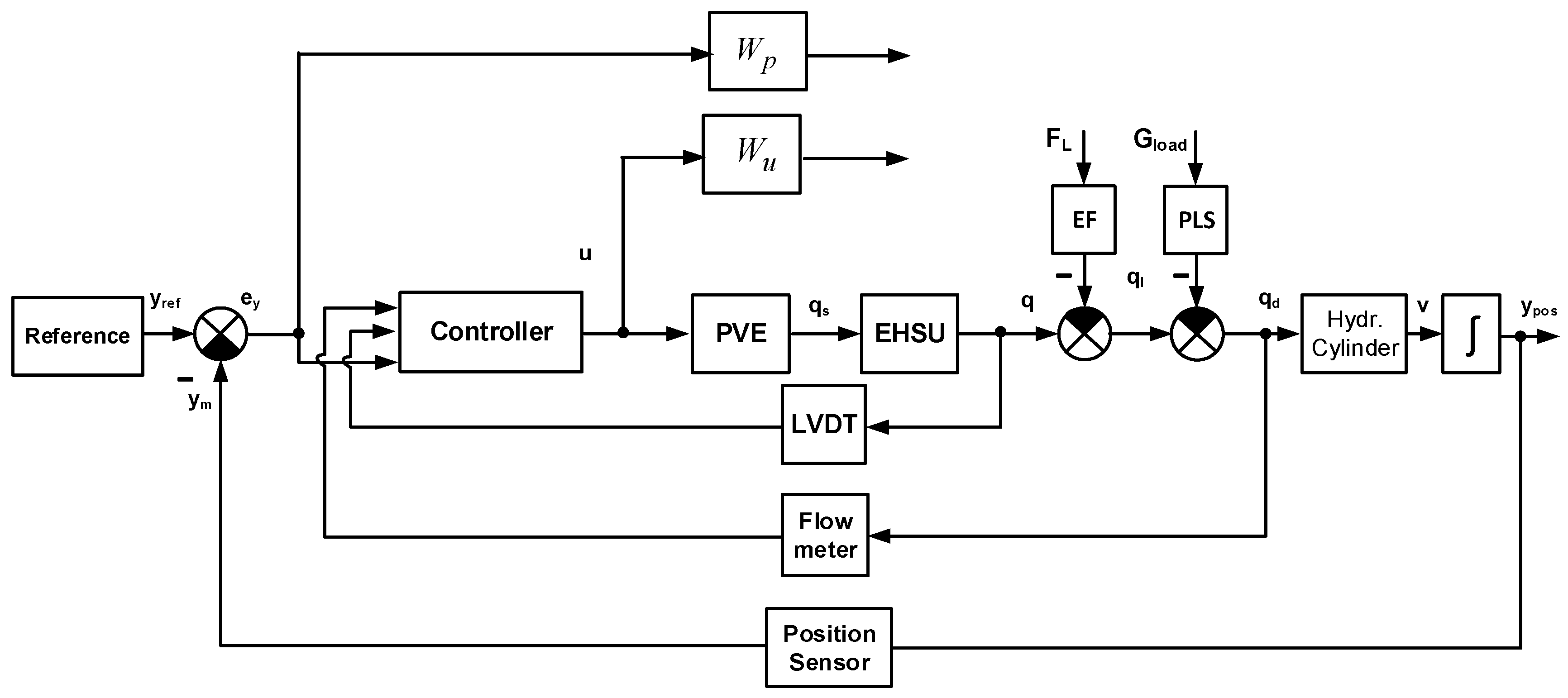
2. Nominal Servo System Model

For the investigation of EHPS, a laboratory test rig for the examination of different types of embedded controllers is designed. The electrohydraulic steering unit (EHSU) introduced into the test rig is OSPEC200 LSRM [16]. The designed hydraulic circuit diagram and detailed description of the test rig system are shown in [17] and real implementation is presented in Figure 1.

In order to design linear multivariable controllers, it is necessary to derive a linear state space model of the plant. In this case, a “black box” type model of an electrohydraulic power steering system is obtained through an identification approach using an experimental dataset. The details on identification were presented in [18]. In this section, only a short representation of the identified model is shown. The system can be modeled sufficiently well by third order state space model with single-input and three outputs. The input is a control action and outputs are the proportional spool position $y_{spool}$, the measured flow rate $y_{flow}$ consumed by the servo cylinder, and the cylinder piston position $y_{pos}$. The first output is measured by the linear variable differential transducer (LVDT), the second is measured by gear flowmeter with coupled encoder and the third output is measured with the linear resistive transducer. The state space form of the estimated plant model is:

$$\begin{array}{l}x(k+1)=A(\theta )x(k)+B(\theta )u(k)+K(\theta )e(k)\\ y(k)=C(\theta )x(k)+D(\theta )u(k)+e(k)\end{array},$$

(1)

where $x={\left[\begin{array}{ccc}{x}_1& x_2& x_3\end{array}\right]}^T$, $y={\left[\begin{array}{ccc}{y}_{spool}& y_{flow}& y_{pos}\end{array}\right]}^T$ are the state vector and the output signal, $\theta$-is the parameters vector and $e={\left[\begin{array}{ccc}{e}_{spool}& e_{flow}& e_{pos}\end{array}\right]}^T$ are the residuals, that are white Gaussian noises. The matrices of the model are:

$$\begin{array}{l}A=\left[\begin{array}{ccc}-1.05& 0.19& 6.27\\ -0.04& 1& 0.198\\ -0.371& 0.033& 2.044\end{array}\right],B={10}^{-3}\left[\begin{array}{c}-0.37\\ -0.034\\ -0.23\end{array}\right],\\ C=\left[\begin{array}{ccc}-31& 0.67& -6.58\\ -0.584& 0.007& -0.25\\ 0.059& -2.019& 0.125\end{array}\right],D={10}^{-3}\left[\begin{array}{c}0.117\\ 0.014\\ 0.0021\end{array}\right].\\ K=\left[\begin{array}{ccc}-0.025& -0.023& -0.022\\ -0.002& 0.0066& -0.429\\ -0.007& -0.01& 0.0033\end{array}\right]\end{array}$$

(2)

Further, the deterministic part of (2) will be regarded as a nominal model and will be used for designing of H_∞ controller and LQG, whereas the stochastic part will be utilized for designing a Kalman filter. It is well known that the designed controllers will ensure nominal stability and performance of the control system, but a priori robust stability and robust performance are not guaranteed. In order to ensure control system performance in presence of disturbances, unmodeled dynamics, non-linearities, and noises the robustness analysis of a closed-loop system should be performed. To achieve this the conservative uncertainty model should be derived.

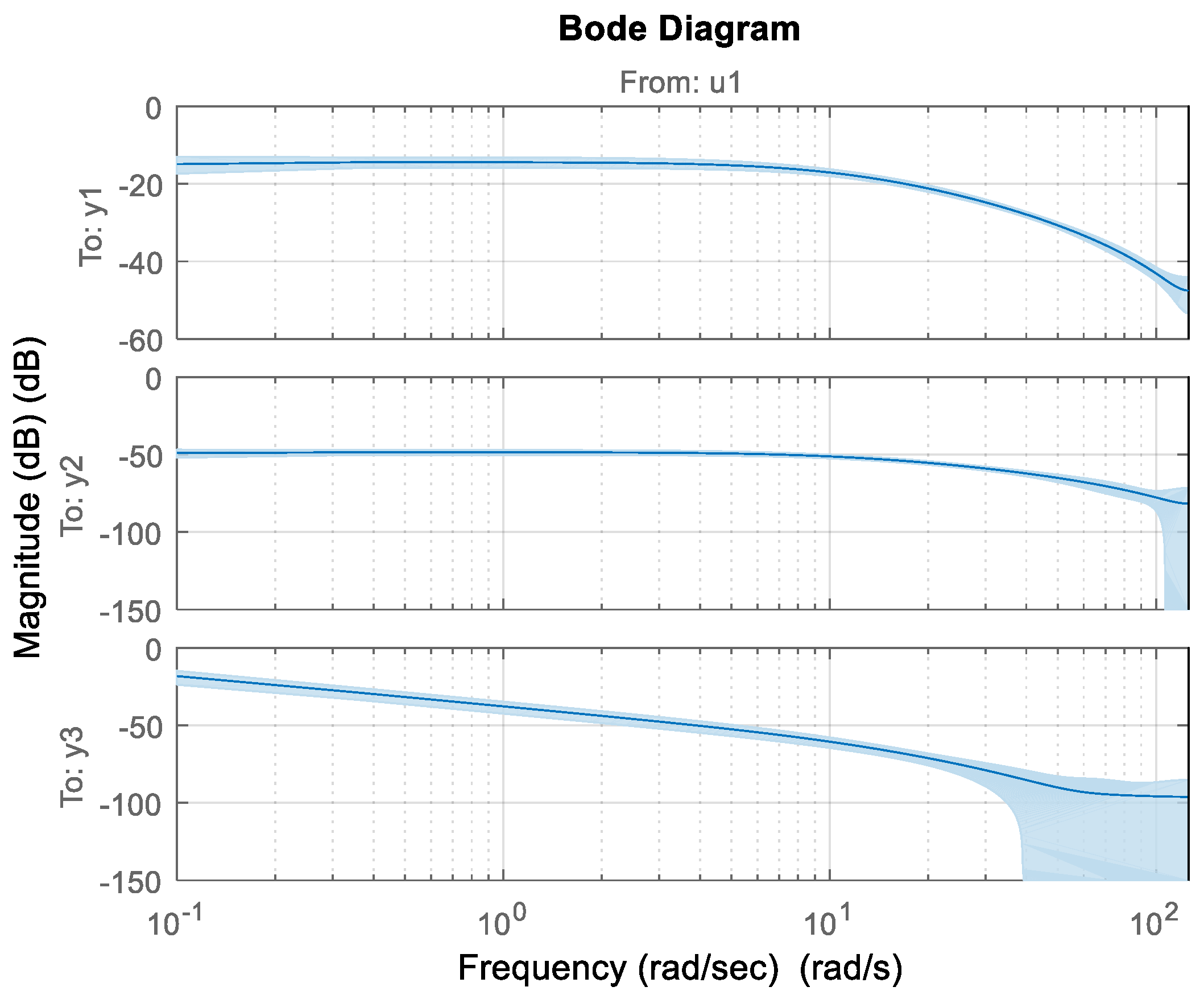
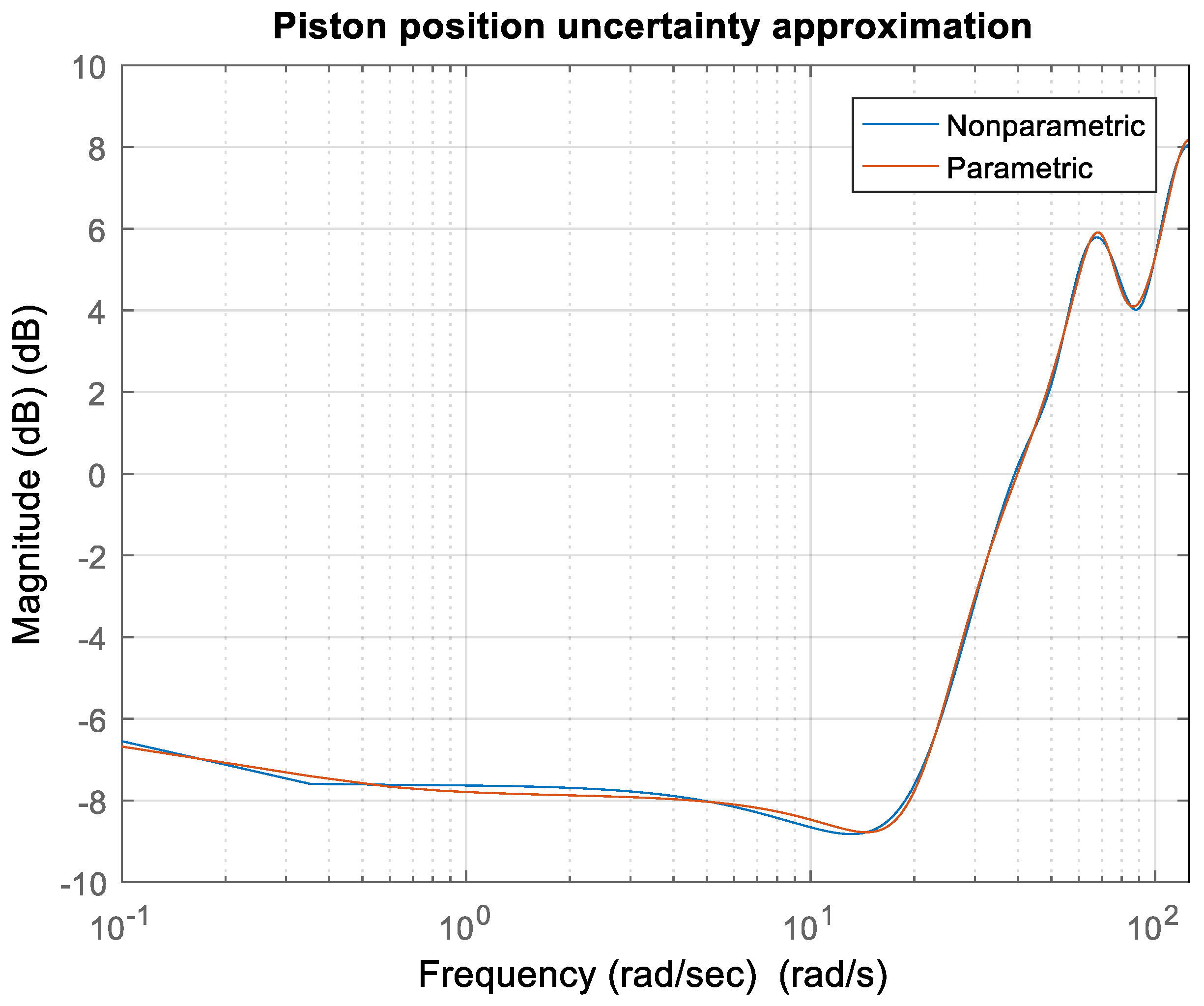
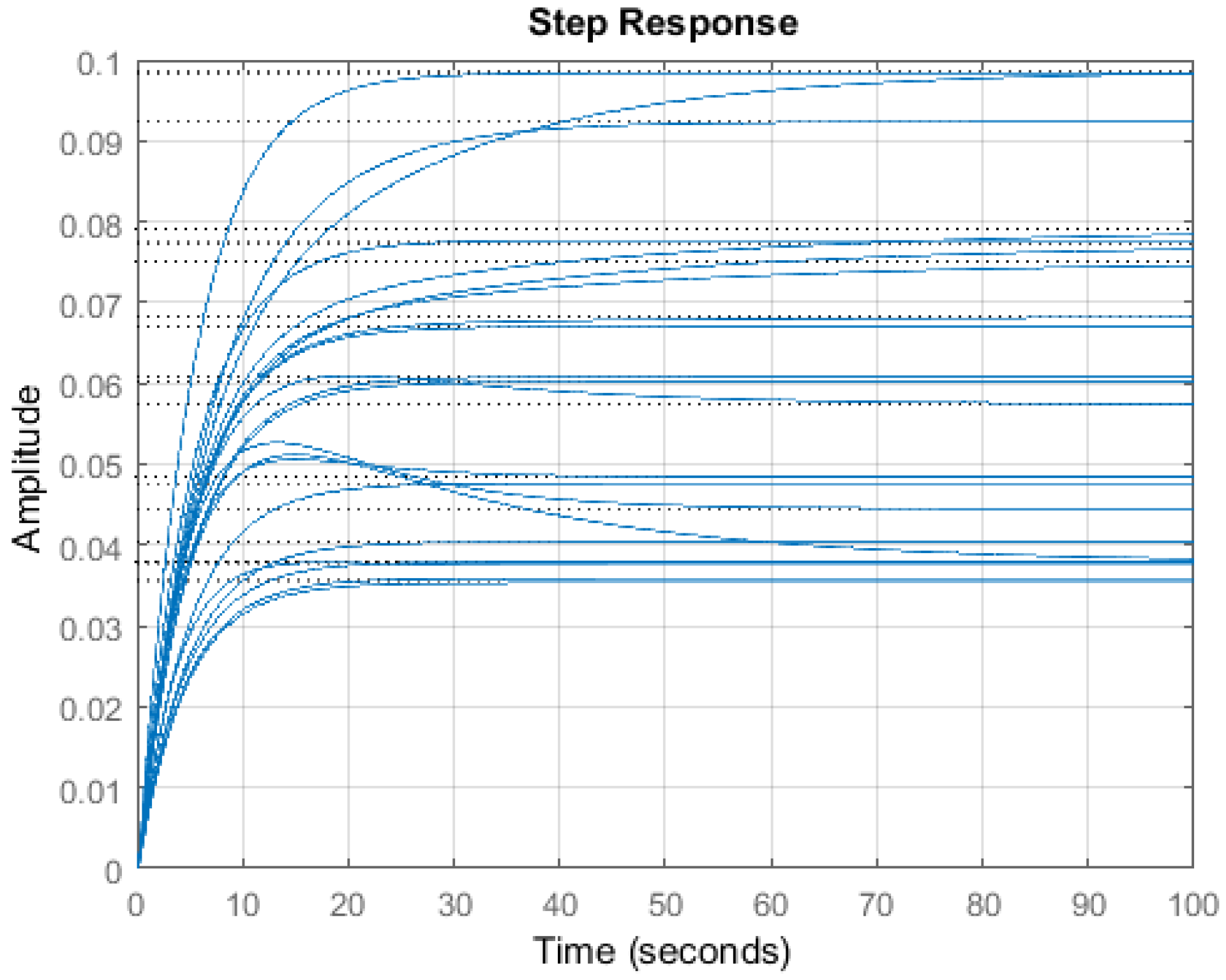
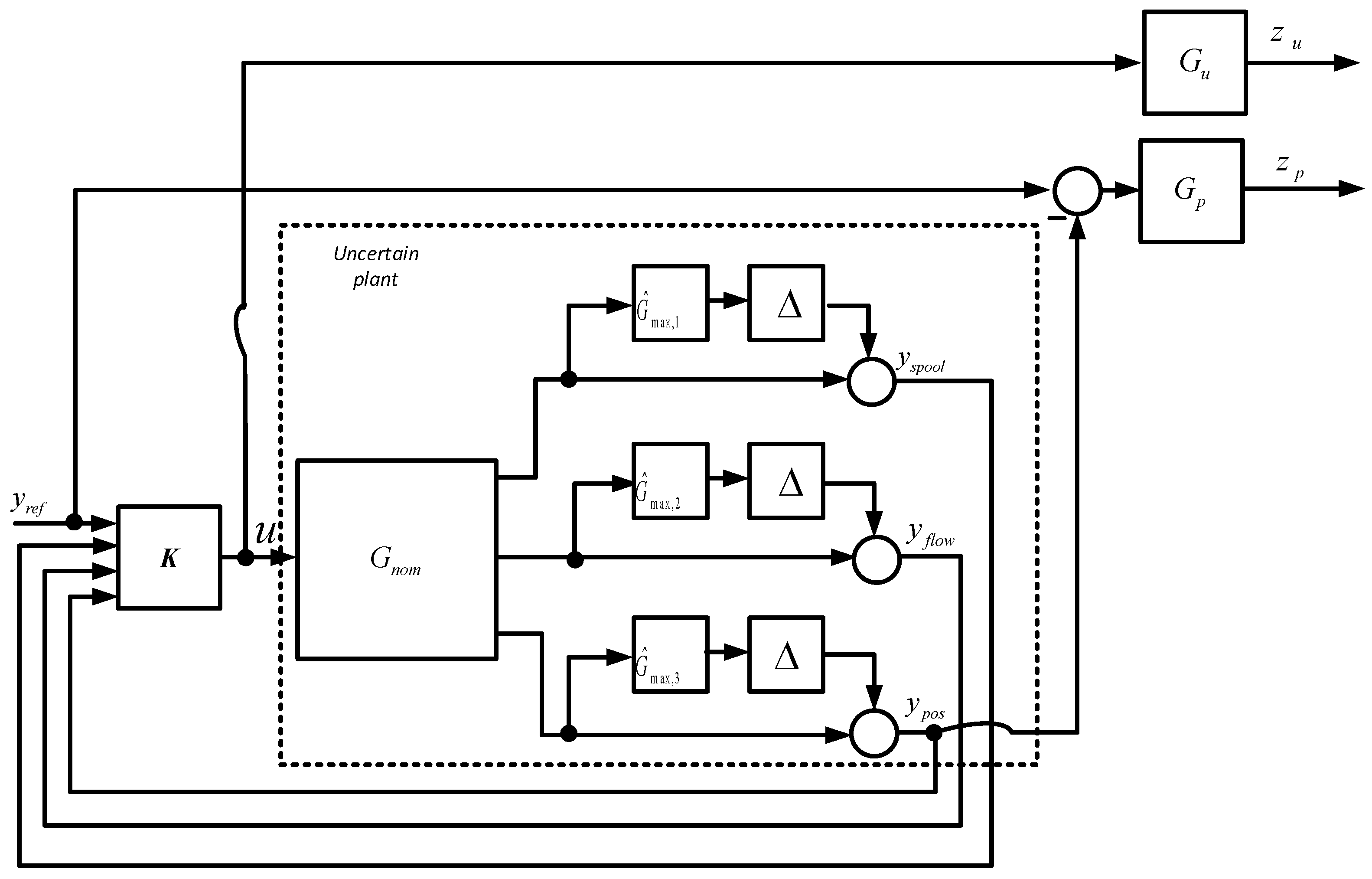
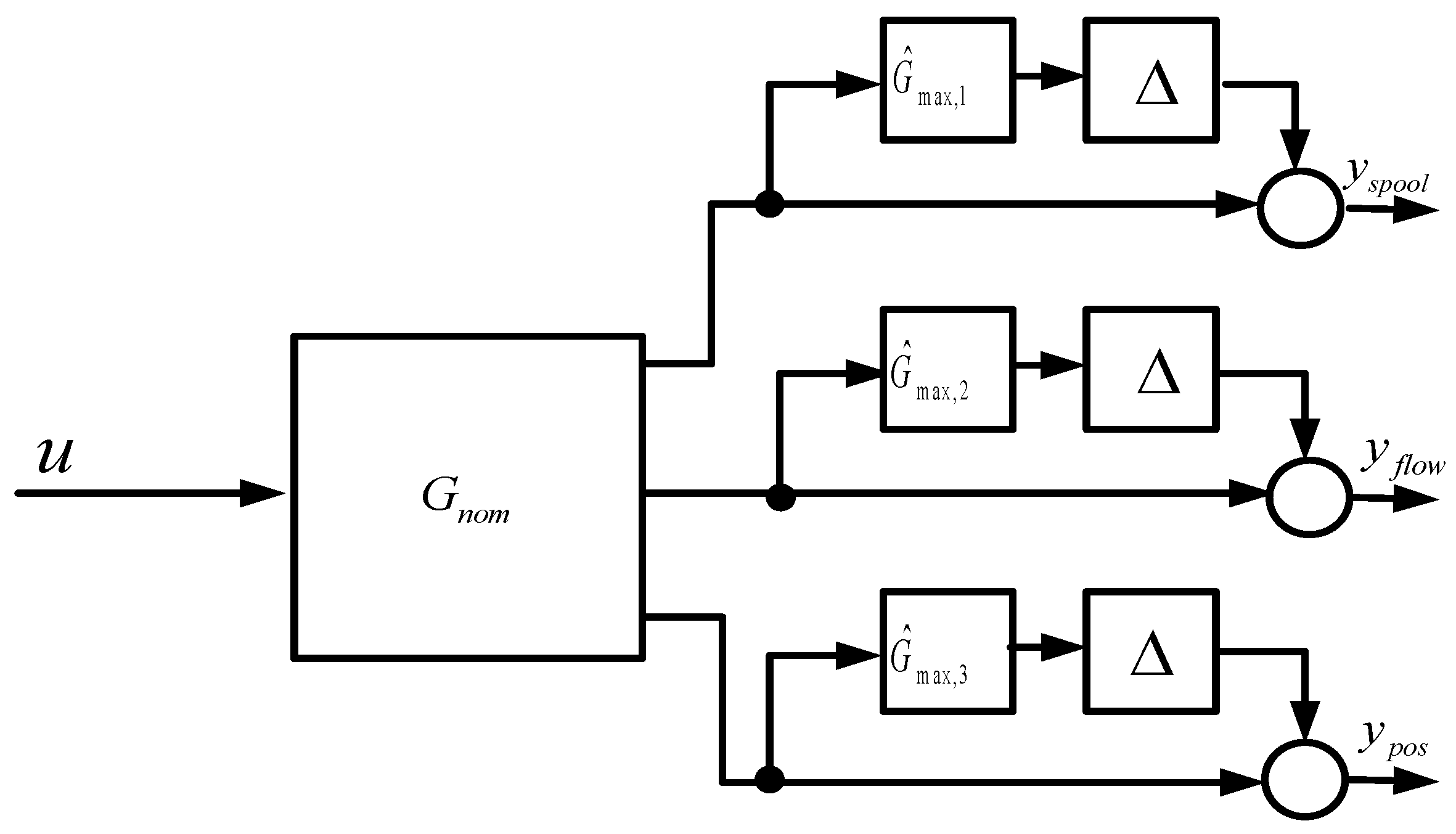
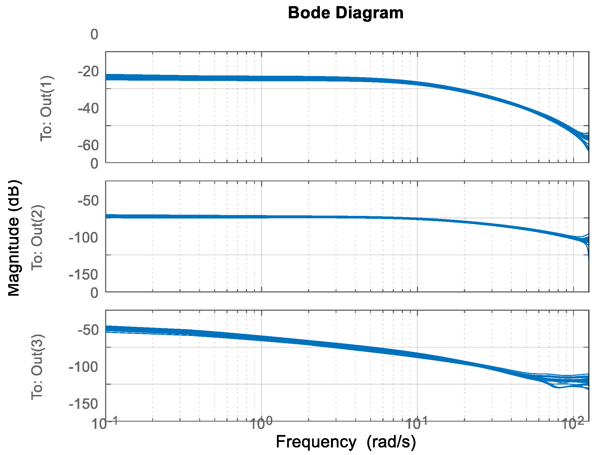
3. Uncertainty Servo System Model

The system identification procedure assumes that the input signal $u\left(k\right)$, output vector $y\left(k\right)$, as well as the residuals $e\left(k\right)$, are zero mean random vectors with Gaussian distribution. Hence, the estimated parameters of the state space model (1) also become random variables with Gaussian distribution. Moreover, the results of residuals correlation tests (Figure 2) show that estimates of parameters are unbiased. This means that the true values of the plant parameters fall in the confidence interval of 3 standard deviations with respect to the nominal values with probability close to 1. Thus, the confidence intervals may be interpreted as parameters uncertainties, which can be used to derive a model with so-called structured uncertainty. However, if the model has many uncertainty parameters there are some difficulties to use it for robust controller design or robustness analysis. In this case, it is more convenient to derive a model with so-called unstructured uncertainties. It is obtained by a representation of parameters uncertainty as uncertainty in closed-loop system frequency responses.

However, the frequency responses are non-linear functions of parameter estimates, but for computing, the uncertainty bounds their first Taylor order approximation is usually taken. For example, the magnitude responses $\left|G_i\left(j\omega ,\theta \right)\right|$ of the identified model, for each of the output channels $i$ can be represented as a random variable with normal distribution. It depends on the standard deviations of the model parameters ${\sigma }_{\theta }$, which give a confidence region around each frequency calculated as

$$\left|G_i\left(i\omega +3{\sigma }_{\theta }\right)\right|=\left|G_{i,nom}\left(i\omega \right)\left(1+G_{\max ,i}\left(j\omega \right){\mathsf{\Delta }}_i\right)\right|,i=1,2,3.$$

(3)

The $G_{\max ,i}\left(j\omega \right)$ and $\left|{\mathsf{\Delta }}_i\left(j\omega \right)\right|<1,i=1,2,3$ are the magnitude response bounds and the scalar uncertainty blocks, respectively. The $G_{i,nom}\left(i\omega \right)$ are transfer functions correspond to the nominal state space model (1). The magnitude responses along with their bounds are presented in Figure 3.

Since the magnitude response bounds $G_{\max ,i}(j\omega )$ are non-parametric functions of frequency, which are inconvenient to use directly in robust stability and robust performance analysis. Hence, a parametric approximation for each of them is constructed with help of the stable minimal phase discrete time transfer functions. For the approximation of the relative uncertainty between the control signal and spool valve, a 5th order transfer function is selected. The approximation is obtained using non-linear least squares optimization which fits the transfer function parameters to match the non-parametric response. The resultant parametric approximation is:

$${\widehat{G}}_{\max ,1}(z)=\frac{0.15(z+0.33)(z-0.82)(z-0.997)(z^2-0.47z+0.51)}{(z+0.78)(z-0.89)(z-0.9995)(z^2-0.25z+0.44)}$$

(4)

The quality of the approximation can be judged from Figure 4, where non-parametric and parametric models are compared for a specific frequency range relevant for the controller’s stability and performance. From a parametric approximation, it is seen that most of the uncertainty in this output channel is in the high frequency domain, however, there is also elevated uncertainty in the low frequency domain, which can be attributed to the dead-band non-linearity of the proportional spool valve.

For the parametric approximation of the relative uncertainty between the control signal and flow rate a 3rd order model with the following discrete time transfer function is used:

$${\widehat{G}}_{\max ,2}(z)=\frac{0.36(z-0.96)(z-0.45)(z+0.19)}{(z+0.84)(z-0.98)(z-0.33)}$$

(5)

As can be seen, the uncertainty in this channel is predominantly in the high frequency range, because the poles and zeros are relatively farther from the unit circle in the z-domain. The fit between non-parametric data and parametric approximation is examined in Figure 5.

Finally, for the parametric approximation of the relative uncertainty bounds between the control signal and the piston position the following transfer function from the 6th order is obtained:

$${\widehat{G}}_{\max ,3}(z)=\frac{1.2(z-0.993)(z-0.19)(z^2-1.43z+0.63)(z^2+0.41z+0.36)}{(z+0.53)(z-0.994)(z^2-1.12z+0.45)(z^2+0.2z+0.52)}$$

(6)

This transfer function also has pronounced high and low frequency components, however, the low frequency part can be mostly neglected due to the proximity between the respective zero and pole pair. The fit between the non-parametric model and its parametric approximation is presented in Figure 6.

Therefore, the final result of the system identification covariance analysis is an approximation of the relative uncertainty bounds $G_{\max ,i}(j\omega )$ with stable discrete time minimal phase transfer function ${\widehat{G}}_{\max ,i}(z)$, where $z=e^{j\omega T_S}$. That allows to map the probability density function over the model set used for system identification to a confidence set of linear systems, or equivalently to an uncertain LTI representation, which in our case utilize a multichannel output multiplicative uncertainty structure presented in Figure 7.

The resultant representation of the uncertain model is:

$$\left(\begin{array}{c}{y}_{spool}(z)\\ y_{flow}(z)\\ y_{pos}(z)\end{array}\right)=\left(\begin{array}{ccc}1+{\widehat{G}}_{\max ,1}(z){\mathsf{\Delta }}_1& 0& 0\\ 0& 1+{\widehat{G}}_{\max ,2}(z){\mathsf{\Delta }}_2& 0\\ 0& 0& 1+{\widehat{G}}_{\max ,3}(z){\mathsf{\Delta }}_3\end{array}\right)G_{non}(z),$$

(7)

where $G_{nom}(z)={\left(\begin{array}{ccc}{G}_{nom,1}(z)& G_{nom,2}(z)& G_{nom,3}(z)\end{array}\right)}^T$ is the transfer matrix corresponding to the SIMO state space model from the system identification represented with expressions (1) and (2). In the above expression, ${\mathsf{\Delta }}_i$ are uncertain SISO transfer functions bounded by norm such that ${\mathsf{\Delta }}_i{}_{\infty }\le 1$.

In Figure 8 and Figure 9, the frequency responses and step responses for 30 random values of plant uncertainty are shown.

As can be seen from the Bode diagram the magnitude responses of the constructed uncertain system with output multiplicative uncertainty are closely matched to bounds of the magnitude response inferred from the system identification.

It should be noted that in the time domain the uncertainty is occurred in time constants and in static gain.

4. Design of LQG and H_∞ Controllers

In previous work, several LQG and H_∞ controllers for electrohydraulic steering systems based on various identification models are developed. These developments are presented in articles [19,20].

Model (2) is used to design the LQG and H_∞ controllers. A detailed description of the procedure for LQG and H_∞ controllers synthesis is presented in [13,14]. The main proposition of this article is the investigation of robust stability and robust performance of the developed embedded electrohydraulic power steering system based on the new uncertainty model. Due to that here only a brief presentation of the controller design procedure is given. The scheme of designed systems is depicted in Figure 10. The block named “Controller” represents designed LQG or H_∞ controllers.

To ensure the performance of reference tracking the integral action LQG controller is designed. For this aim, the nominal model (2) is modified as

$$e_{\mathrm{int},pos}(k+1)=e_{\mathrm{int},pos}(k)+T_s{e}_{pos}(k), e_{pos}(k)=T_s(y_{ref}(k)-y_{pos}(k)),$$

(8)

where $y_{ref}(k)$ is the reference of cylinder piston position, $T_s=0.01s$—the sample time, $e_{\mathrm{int},pos}(k)$—the discrete time integral of cylinder piston position error, and $e_{pos}(k)$—the cylinder piston position error. Combining model (1) and Equation (8) the description of the augmented plant is obtained as

$$\begin{array}{l}\overline{x}(k+1)=\overline{A}\overline{x}(k)+\overline{B}u(k)+\overline{G}{y}_{ref}(k),\\ y(k)=\overline{C}\overline{x}(k),\end{array}$$

(9)

where $\overline{x}(k)=\left|\begin{array}{c}x(k)\\ e_{\mathrm{int},pos}(k)\end{array}\right|,\overline{A}=\left|\begin{array}{cc}A& 0\\ -T_{s}C& 1\end{array}\right|,\overline{B}=\left|\begin{array}{c}B\\ 0\end{array}\right|,\overline{C}=\left|\begin{array}{cc}C& 0\end{array}\right|,\overline{G}=\left|\begin{array}{c}0\\ T_s\end{array}\right|$. The controller formed control signal as:

$$u(k)=-K_c\widehat{x}(k)-K_i{e}_{\mathrm{int},pos}(k)$$

(10)

where $K_c$ and $K_i$ are the proportional and integral parts of the controller. The state estimates $\widehat{x}(k)$ are computed by the Kalman filter.

$$\widehat{x}(k+1)=A\widehat{x}(k)+Bu(k)+K_f(y(k+1)-CBu(k)-CA\widehat{x}(k))$$

(11)

where $K_f$ is matrix Kalman filter gain. It is obtained by MATLAB^® function Kalman [21]. The covariance of residual in the model (1) is used in the Kalman filter design procedure.

The obtained LQG controller minimizes performance criteria [22]

$$J(u)={\displaystyle \sum _{k=0}^{\infty }{\overline{x}}^T(k)Q\overline{x}(k)+u^T(k)Ru(k)}$$

(12)

where $Q=\left[\begin{array}{cc}1000& 0\\ 0& 500C_3^T{C}_3\end{array}\right]$, $R=100$ and $C_3$ is the third row of a matrix $C$.

In order to design H_∞ controller, two weighting transfer functions $W_p$, $W_u$ and are introduced. They are used to specify the performance requirements for the closed loop control system. Thus the plant description used in the design of H_∞ controller is

$$x_{ext}(k+1)=A_{ext}{x}_{ext}(k)+B_{ext}\left(\begin{array}{c}e\\ y_{ref}\\ u\end{array}\right),\left(\begin{array}{c}{z}_u\\ z_y\\ y_{cont}\end{array}\right)=C_{ext}{x}_{ext}+D_{ext}\left(\begin{array}{c}e\\ y_{ref}\\ u\end{array}\right)$$

(13)

where $x_{ext}=\left[x_1,x_2,x_3,x_u,x_p\right]$, $x_u$ and $x_p$ are the states corresponding to $W_p$, $W_u$ and $y_{cont}={[\begin{array}{ccc}{y}_{spool}& y_{flow}& e_{pos}\end{array}]}^T$ is the input of H_∞ controller. The controller parameters are determined by solving the mixed sensitivity optimization problem [23]

$$\min {\Vert \begin{array}{c}{W}_{p}S\\ W_{u}KS\end{array}\Vert }_{\infty }<\gamma$$

(14)

where $\gamma >0$, $S$ is the output sensitivity function and $K$ is the controller transfer matrix. It is known that in practice a suboptimal H_∞ controller is obtained. If after optimization $\gamma$ in (14) is smaller than 1, this means that the prescribed by weighting transfer functions nominal system performance is achieved. The controller design is performed for weighting functions

$$W_p=\frac{0.3(0.001s+1)}{300s+1},W_u=\frac{0.001(0.3s+1)}{0.001s+1}.$$

(15)

The obtained value for $\gamma$ is 0.5387, which guarantees nominal performance. The step responses of nominal systems with both controllers are depicted in Figure 11.

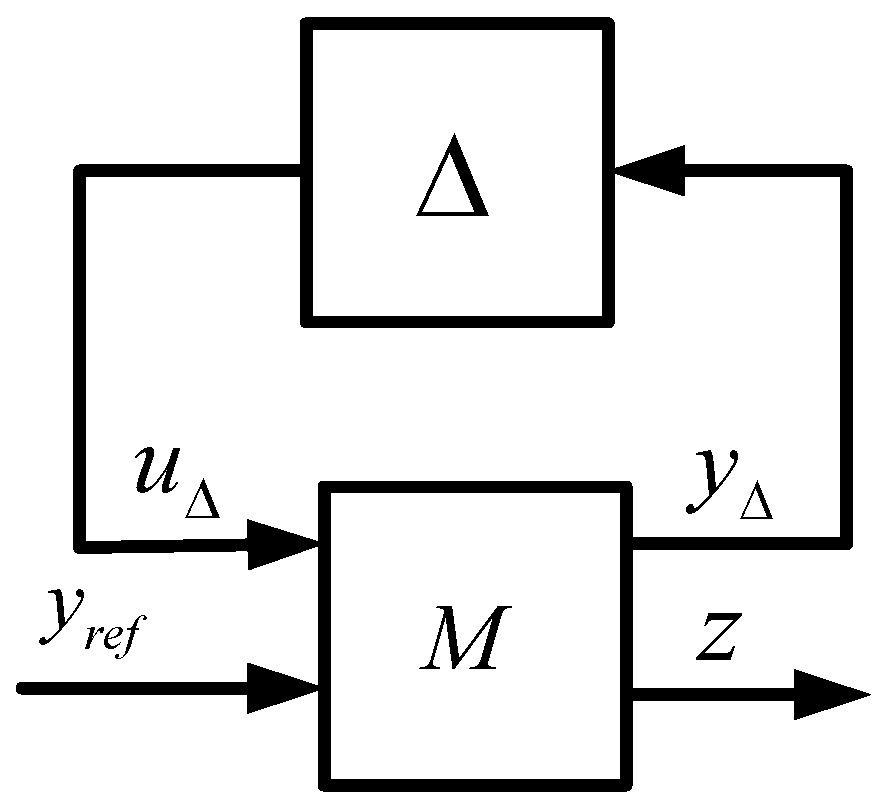
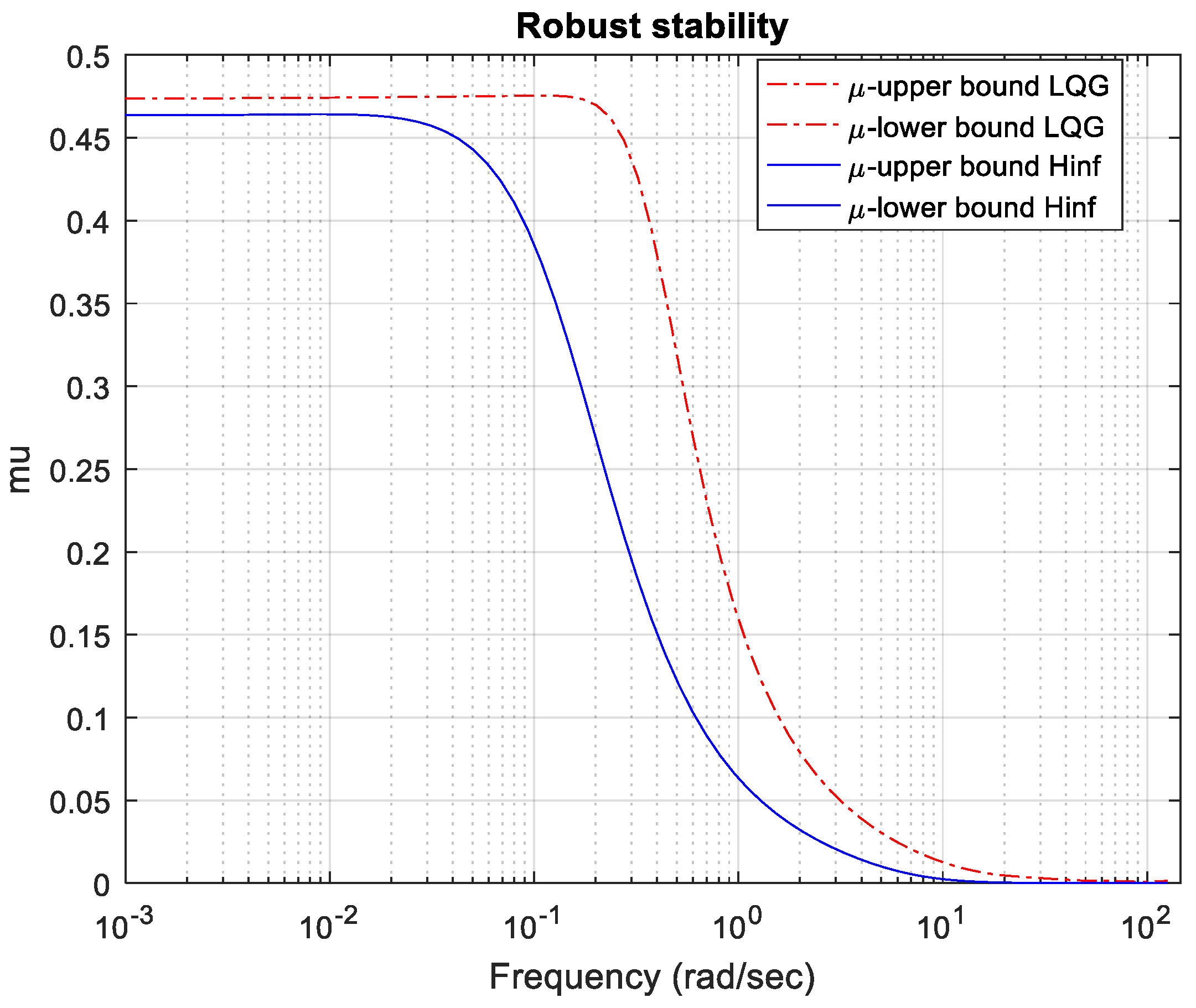
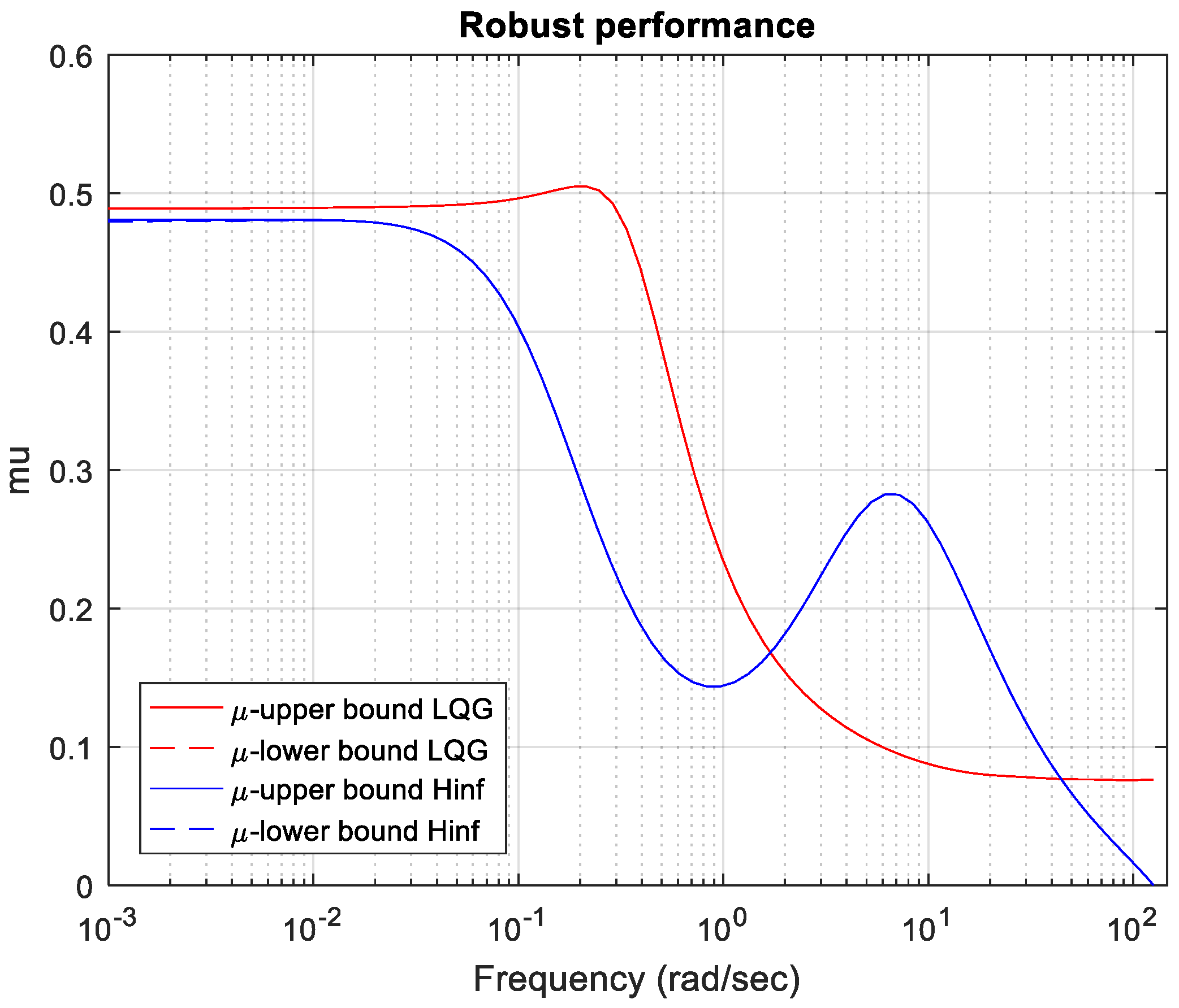
5. Robust Stability and Robust Performance Analysis

The block diagram of a closed-loop system with the uncertain model (7) that is used for robust stability and robust performance analysis is presented in Figure 12. The block named $K$ is the transfer matrix of designed LQG or H_∞ controllers. In order to investigate the robust stability, it is convenient to transform the structure scheme of the control system from Figure 12 to the standard $M-\mathsf{\Delta }$ structure, depicted in Figure 13. In this loop $y_{\mathsf{\Delta }}$ is the uncertainty output, $z={\left[\begin{array}{cc}{z}_u& z_p\end{array}\right]}^T$ is the external (performance) output, and $u_{\mathsf{\Delta }}$ is the uncertainty input. In case of robust stability analysis $z_u=u$$z_p=y_{ref}-y_{pos}$ and. The block named $M$ is a lower Linear Fractional Transformation of nominal plant $G_{nom}$ and controller $K$

$$M=F_l(P,K).$$

(16)

The system depicted in Figure 13 achieved robust stability for all $\mathsf{\Delta }$ if, and only if, [12,24]:

$${\mu }_{\mathsf{\Delta }}[F_l(G_{nom},K)]<1,$$

(17)

where ${\mu }_{\mathsf{\Delta }}[F_l(G_{nom},K)]$ is the structure singular value of the closed-loop system. The robust performance of the control system with both controllers is investigated for weighting functions (15).

The robust performance test is performed concerning an extended uncertain structure. For the designed control system the extended uncertain structure, take a form:

$${\mathsf{\Delta }}_{G_{nom}}=\left\{\left[\begin{array}{cc}\mathsf{\Delta }& 0\\ 0& {\mathsf{\Delta }}_F\end{array}\right]:{\mathsf{\Delta }}_F\in C^{1\times 2}\right\}$$

(18)

where ${\mathsf{\Delta }}_F$ is a fictitious complex uncertainty with two inputs $z_u$ and $z_p$, and one output $y_{ref}$. The system with controller $K$ reach robust performance if, and only if,

$${\mu }_{{\mathsf{\Delta }}_{Gnom}}\left[F_l\left(G_{nom},K\right)\left(j\omega \right)\right]<1$$

(19)

where ${\mu }_{{\mathsf{\Delta }}_{Gnom}}\left[F_l\left(G_{nom},K\right)\left(j\omega \right)\right]<1$ is the structured singular value evaluated with respect in the extended uncertainty (18).

In Figure 14 the limits of structured singular value (17) for both control systems are presented. It is seen that both closed-loop systems are robustly stable. Both systems can tolerate approximately up to 215% of the modeled uncertainty. For both controllers the sensitivity concerning uncertainty is mostly due to ${\mathsf{\Delta }}_3\left(j\omega \right)$, for example, 25% increasing in this uncertain element leads to a 25% decreasing in the stability margin. The sensitivity of stability margin with respect to ${\mathsf{\Delta }}_1\left(j\omega \right)$ or ${\mathsf{\Delta }}_2\left(j\omega \right)$ is negligible. That can be explained with the presence of an additional integrator concerning piston position channel.

In Figure 15, the bounds of structured singular value (19) for both control systems are presented. It is seen that both systems achieved robust performance. The system with H_∞ controller is more robust than the one with LQG controller. The system with H_∞ controller can tolerate up to 208% of the modeled uncertainty without losing robust performance, whereas the system with LQG controller can tolerate up to 192% of modeled uncertainty. Again, the sensitivity of the performance margin concerning the uncertainty ${\mathsf{\Delta }}_3\left(j\omega \right)$ (piton position) is highest. This means that the third output is most important for control system performance.

In Figure 16, the step responses of both closed-loop systems for 50 random values of plant uncertainty are shown. As can be seen, the step responses are close to these of nominal closed-loop systems (see Figure 11), which again confirm the robust performance of designed systems. The transient response of the system with LQG has a negligible overshoot of approximately 5%, whereas the ones of the system with H_∞ controller do not have an overshoot.

In Figure 17 and Figure 18, the position sensitivity and position complementary sensitivity for 50 random values of plant uncertainty are shown. The bandwidth of the system with LQG controller is a bit wider than one of the system with H_∞ controller. Again, it is seen robustness of both closed-loop systems.

The disturbance attenuation for both systems is close. For instance, the disturbance with a frequency of 0.01 rad/s will be suppressed 10 times by the system with H_∞ controller and 12 times by the system with LQG controller. The bandwidth of the LQG system is wider than one of system with H_∞ controller.

In Figure 19, the control signal sensitivity to noise of the designed control systems for 50 random values of plant uncertainty are shown. The LQG controller is more sensitive to noises than H_∞ controllers. This means that the real control signal of the system with LQG controller may have more oscillations than the one for a control system with H_∞ controller, which influences on system’s energy efficiency.

The quantitative analysis of the performance of both control systems in frequency and time domain is performed. It is based on the maximal and minimal values of the following indices which are evaluated for 50 random values of plant uncertainty:

Maximal and minimal values of H_∞ norm:

$$M_s={\Vert \left|S(j\omega )\right|\Vert }_{\infty }$$

(20)

where $\left|S(j\omega )\right|$ is output sensitivity of the closed-loop system.

Maximal and minimal closed-loop bandwidth ${\omega }_{BT}$. The ${\omega }_{BT}$ is defined as the frequency at which complementary sensitivity $\left|T(j\omega )\right|$ concerning cylinder piston position crosses the line −3 db from above.

Maximal and minimal overshoot:

$$\sigma =\frac{y_{pos,\max }-y_{pos}(\infty )}{y_{pos}(\infty )}100,\%$$

(21)

where $y_{pos,\max }$ is the first peak of the transient response with respect to cylinder piston position and $y_{pos}(\infty )$ is its steady state value.

Maximal and minimal settling time $t_s$. It is defined as the minimum period of time after which the cylinder piston position remains within 5% of its steady state value.

The maximal and minimal square root of integral error with respect to cylinder piston position:

$$J_e=\sqrt{\frac{1}{N}{\displaystyle \sum _{i=0}^{N-1}{(r(i)-y_{pos}(i))}^2}}$$

(22)

The maximal and minimal values of above described indices for both control systems are given in

Table 1. Performance indices obtained by Monte Carlo simulation.

	${\mathit{M}}_{\mathit{S},\mathbf{max}}$	${\mathit{M}}_{\mathit{S},\mathbf{min}}$	${\mathit{\omega }}_{\mathit{B}\mathit{T},\mathbf{max}}$	${\mathit{\omega }}_{\mathit{B}\mathit{T},\mathbf{min}}$	${\mathit{\sigma }}_{\mathbf{max}}$	${\mathit{\sigma }}_{\mathbf{min}}$	${\mathit{t}}_{\mathit{s}\mathit{t},\mathbf{max}}$	${\mathit{t}}_{\mathit{s}\mathit{t},\mathbf{min}}$	${\mathit{J}}_{\mathit{e},\mathbf{max}}$	${\mathit{J}}_{\mathit{e},\mathbf{min}}$
	dB	dB	rad/s	rad/s	%	%	s	s	mm	mm
LQG	2.5	1.8	0.36	0.27	6.5	0.1	16.00	12.00	12.07	10.61
$H_{\infty }$	0.5	0.3	0.2	0.1	0	0	30	16.4	14.79	11.12

. They are evaluated according to 50 random values of plant uncertainty, which are obtained by Monte Carlo simulation.

It is seen that the difference between maximal and minimal values of corresponding indices are small for both control systems, which show their robustness. Only one exclusion can be seen for the settling time of H_∞ system, where the difference between maximal and minimal settling time is approximately equal to the minimal value. However, this system has not overshoot in transient response.

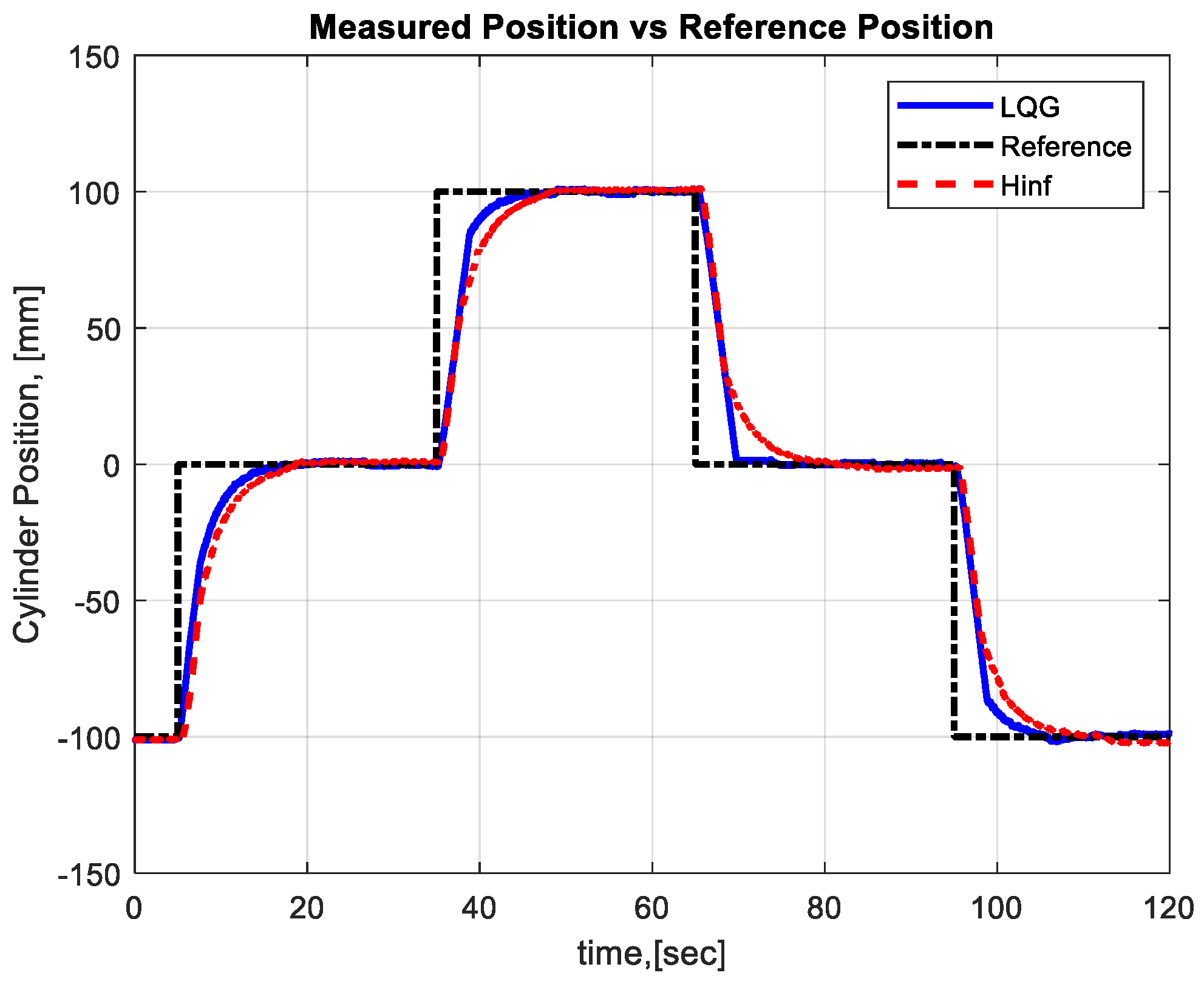
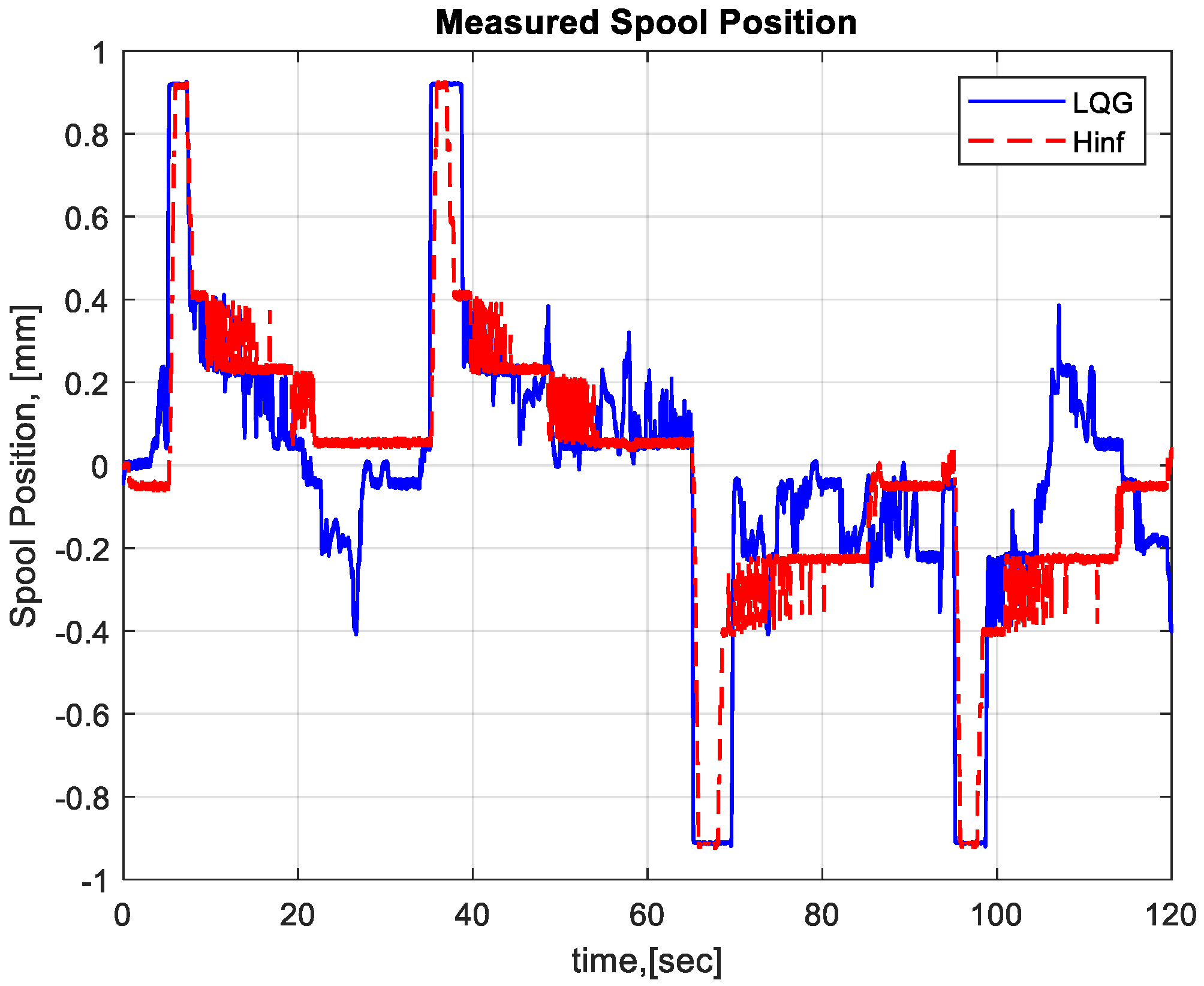
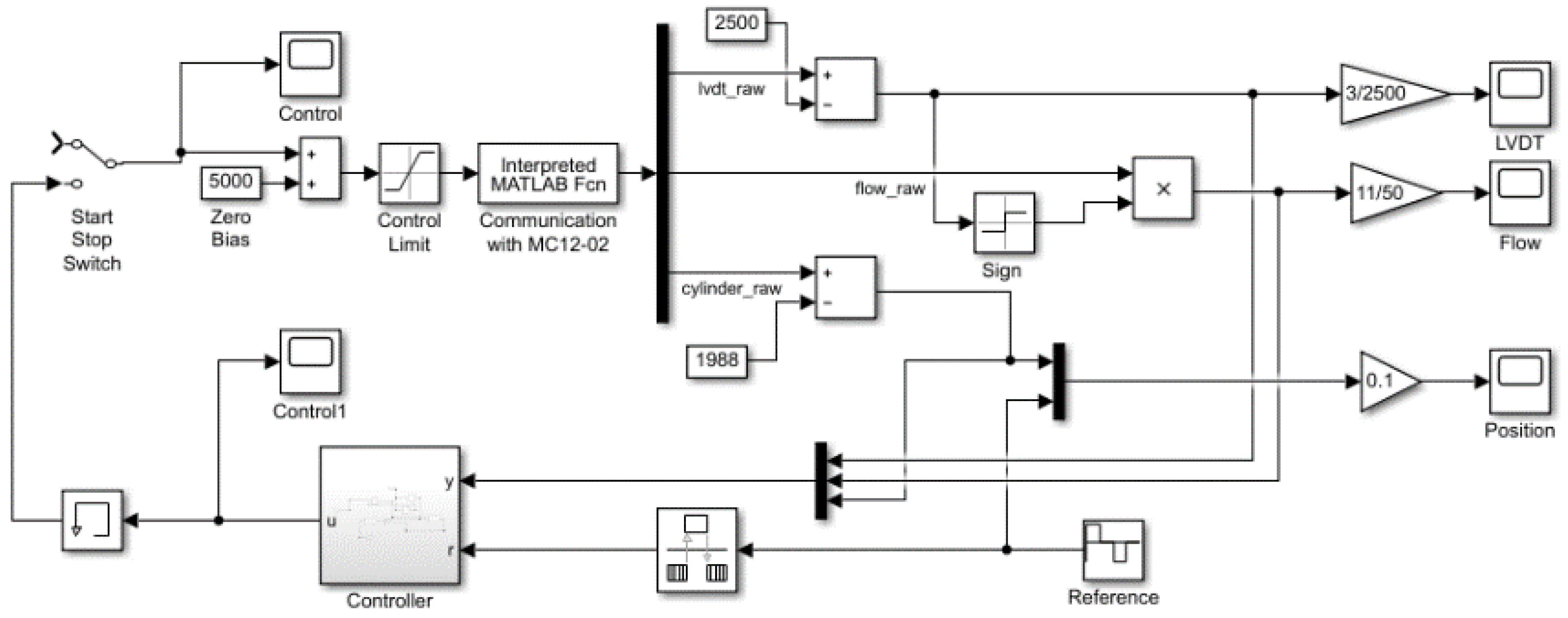
6. Experimental Results for Performance Verification

The developed real time Simulink^® structure used for experiments with LQG and $H_{\infty }$ controllers is presented in Figure 20 [14]. The main block in the model is the MATLAB^® function block which realizes the communication on the CAN channel between the microcontroller MC012-022 [25] and the workstation. A more detail description of the developed laboratory test rig for examination of different types of embedded controllers can be found in [16]. Here, in order to approve obtained results for the robustness of control systems, we briefly give some experimental results for both control systems.

Figure 21 compares the transient response of the steering cylinder piston obtained with both controllers (LQG and H_∞). These experiments confirm the observation from the simulation that both controllers share similar performance in terms of settling time and steady state accuracy (settling time for the LQG system is approximately 12 s, as one for H_∞ system is 15 s). Both controllers do not overshoot, but the LQG has a faster response in both directions, that is according to its wider bandwidth (see Figure 17).

The comparison between control signals obtained with both closed-loop systems is presented in Figure 22. As can be seen, the amplitude of the control signal of the LQG system is higher than one of the H_∞ system. In a steady state regime, the control signal of the H_∞ system is less oscillatory than LQG one, which can be explained by its lower sensitivity to output disturbances (see Figure 19). The energy necessary to control an EHPS unit with a H_∞ controller is significantly less than one to control unit with LQG controller.

Figure 23 and Figure 24 compare the internal system variables—flow rate and spool position. It can be observed that both controllers affect on flow rate and spool position. On the other side, there is strong relation between both variables, which indicates the accuracy of the proportional spool valve.

In

Table 2. Performance indices obtained by experimental results.

	$\mathit{\sigma }$	$\mathit{t}$	$\mathit{J}$
	%	s	mm
LQG	0	10.00	732.5
$H_{\infty }$	0	14.4	885.7

some of the performance indices of both systems obtained via experimental data are shown.

It is seen that both system has similar performance, which in accordance with the analysis made in the previous section.

7. Conclusions

The article presents the developed approach for robust stability and the robust performance investigation of an embedded system for control of electrohydraulic power steering based on two different advanced control strategies—linear-quadratic Gaussian (LQG) and H_∞. The approach uses the framework of structured singular value $\mu$ that is one of the basic tool for analysis in robust control theory. In contrast with existing approaches for robustness analysis of EHPS control systems, the analysis in this article is performed via the new uncertainty SIMO model of the EHPS unit. The uncertainty in this model is obtained via experimental data and it is more realistic than one in existing uncertainty models of the EHPS unit. In such a manner, the new model takes into account the effects of unmodeled dynamics, non-linearities, disturbances, and measurement noises to the control system performance. The obtained results show that both control systems achieved robust stability and performance with similar robust stability and performance margins. In order to approve theoretical results, the designed controllers are implemented in the PLC and real experiments of the EHPS unit control system are performed. They confirm the robustness of the closed-loop system and are similar to the results obtained via simulation analysis. The assessment of the control performance is derived on the basis of performance indices (see Table 1 and Table 2). A comparative analysis of these indices for LQG and H_∞ controller obtained from the simulation and experimental results is made. The results of this analysis once again confirm the robustness of the developed embedded system with both advanced control techniques.

References

1. Milić, V.; Šitum, Ž.; Essert, M. Robust H position control synthesis of an electro-hydraulic servo system. ISA Trans. 2010, 49, 535–542. [Google Scholar] [CrossRef] [PubMed]
2. Proca, A.; Keyhani, A. Identification of Power Steering System Dynamic Models. Mechatronics 1998, 8, 255–270. [Google Scholar] [CrossRef]
3. Más, F.; Zhang, Q.; Hansen, A.C. Mechatronics and Intelligent Systems for Off-Road Vehicles; Springer: London, UK, 2010. [Google Scholar]
4. Qiu, H.; Zhang, Q. Feedforward-plus-proportional-integral-derivative controller for an off-road vehicle electrohydraulic steering system. Proc. Inst. Mech. Eng. Part D J. Automob. Eng. 2017, 2003, 375–382. [Google Scholar] [CrossRef]
5. Atherton, D.P.; Majhi, S. Limitations of PID Controllers. In Proceedings of the 1999 American Control Conference, San Diego, CA, USA, 2–4 June 1999; Volume 6, pp. 3343–3847. [Google Scholar]
6. Åström, K.; Hägglund, T. The Future of PID Control. Control Eng. Pract. 2001, 9, 1163–1175. [Google Scholar] [CrossRef]
7. Jin, Z.; Zhang, L.; Zhang, J.; Khajepour, A. Stability and optimized H control of tripped and untripped vehicle rollover. Veh. Syst. Dyn. 2016, 54, 1405–1427. [Google Scholar] [CrossRef]
8. Wang, C.; Deng, K.; Zhao, W.; Zhou, G.; Zhou, D. Stability control of steer by wire system based on μ synthesis robust control. Sci. China Technol. Sci. 2017, 60, 16–26. [Google Scholar] [CrossRef]
9. Min, Y.; Quan, W.; Shengjie, J. Robust H2/H Control for the Electrohydraulic Steering System of a Four-Wheel Vehicle. Math. Probl. Eng. 2014, 4, 1–12. [Google Scholar]
10. Zhao, W.; Li, Y.; Wang, C.; Zhao, T.; Gu, X. H control of novel active steering integrated with electric power steering function. J. Cent. South Univ. 2013, 20, 2151–2157. [Google Scholar] [CrossRef]
11. Dannöhl, C.; Müller, S.; Ulbrich, H. H-control of a rack-assisted electric power steering system. Int. J. Veh. Mech. Mobil. 2012, 50, 527–544. [Google Scholar] [CrossRef]
12. Petkov, P.; Slavov, T.S.; Kralev, J. Design of Embedded Robust Control Systems Using MATLAB®/Simulink®; The Institution of Engineering and Technology: London, UK, 2018. [Google Scholar]
13. Mitov, A.L.; Kralev, J.; Slavov, T.S.; Angelov, I.L. Reference Tracking LQG Control of Electrohydraulic Servo System for Mobile Machines. In Proceedings of the 10th IEEE International Conference on Intelligent Systems, Varna, Bulgaria, 26–28 June 2020; pp. 475–480. [Google Scholar]
14. Mitov, A.L.; Kralev, J.; Slavov, T.S.; Angelov, I.L. Design of H-infinity Tracking Controller for Application in Autonomous Steering of Mobile Machines. In Proceedings of the 19th International Scientific Conference Engineering for Rural Development, Jelgava, Latvia, 20–22 May 2020; pp. 871–876. [Google Scholar]
15. Mitov, A.; Slavov, T.; Kralev, J.; Angelov, I. Lecture Notes of the Institute for Computer Sciences, Social-Informatics and Telecommunications Engineering, LNICST. In Robust Stability and Performance Investigation of Electrohydraulic Steering Control System; Springer: Berlin/Heidelberger, Germany, 2021; Volume 382, pp. 386–400. [Google Scholar]
16. Danfoss Inc. OSPE Steering Valve. Technical Information. 11068682. November 2016. Available online: https://www.sauerbibus.de/fileadmin/editors/countries/sab/Produkte/Danfoss_Neu/Lenkungskomponenten/OSPE_Steering_Valve_Technical_Information_englisch.pdf (accessed on 25 September 2021).
17. Angelov, I.; Mitov, A. Test Bench for Experimental Research and Identification of Electrohydraulic Steering Units. In Proceedings of the 10th International Fluid Power Conference, Dresden, Germany, 8–10 March 2016; pp. 225–236. [Google Scholar]
18. Mitov, A.L.; Kralev, J.; Slavov, T.S.; Angelov, I.L. SIMO System Identification of Transfer Function Model for Electrohydraulic Power Steering. In Proceedings of the 16th International Conference on Electrical Machines, Drives and Power Systems (ELMA), Sofia, Bulgaria, 6–8 June 2019; pp. 130–135. [Google Scholar]
19. Slavov, T.S.; Mitov, A.L.; Kralev, J. Advanced Embedded Control of Electrohydraulic Power Steering System. Cybern. Inf. Technol. 2020, 20, 105–121. [Google Scholar] [CrossRef]
20. Mitov, A.L.; Slavov, T.S.; Kralev, J.; Angelov, I.L. Comparison of Robust Stability for Electrohydraulic Steering Control System Based on LQG and H-infinity Controller. In Proceedings of the 42st International Conference on Telecommunications and Signal Processing TSP, Budapest, Hungary, 1–3 July 2019; pp. 712–715. [Google Scholar]
21. The Mathworks Inc. Control System Toolbox. In User’s Guide; The Mathworks Inc.: Portola Valley, CA, USA, 2016. [Google Scholar]
22. Goodwin, G.; Graebe, S.; Salgado, M. Control System Design; Prentice Hall: Upper Saddle River, NJ, USA, 2001. [Google Scholar]
23. The Mathworks Inc. Robust Control Toolbox. In User’s Guide; The Mathworks Inc.: Portola Valley, CA, USA, 2016. [Google Scholar]
24. Zhou, K.; Doyle, J. Robust and Optimal Control; Prentice Hall International: Upper Saddle River, NJ, USA, 1996. [Google Scholar]
25. Danfoss Inc. Plus+1 Controllers MC012-020 and 022. Data Sheet, 11077167. September 2013. Available online: https://www.danfoss.com/en/products/dps/electronic-controls/controllers/plus1-controllers/plus1-mc-microcontrollers/#tab-documents (accessed on 25 September 2021).
Figure 1. The real implementation of laboratory electrohydraulic power steering test rig.
Information 12 00512 g001
Figure 2. Residuals correlation test.
Information 12 00512 g002
Figure 3. Frequency responses with their maximal deviations.
Information 12 00512 g003
Figure 4. Approximation of the relative uncertainty in the spool position.
Information 12 00512 g004
Figure 5. Approximation of the relative uncertainty in the flow rate.
Information 12 00512 g005
Figure 6. Approximation of the relative uncertainty in the piston position.
Information 12 00512 g006
Figure 7. The obtained model with output multiplicative uncertainty.
Information 12 00512 g007
Figure 8. Frequency responses of uncertainty model.
Information 12 00512 g008
Figure 9. Step responses of the uncertain model.
Information 12 00512 g009
Figure 10. Structure of closed-loop system.
Information 12 00512 g010
Figure 11. Step responses of nominal closed-loop systems.
Information 12 00512 g011
Figure 12. Block diagram of the closed-loop system with the uncertain plant.
Information 12 00512 g012
Figure 13. M—Δ Representation of EHPS.
Information 12 00512 g013
Figure 14. µ bounds for robust stability analysis.
Information 12 00512 g014
Figure 15. µ bounds for robust performance analysis.
Information 12 00512 g015
Figure 16. Transient characteristics with respect to the cylinder piston position.
Information 12 00512 g016
Figure 17. The sensitivity of cylinder piston position to disturbances.
Information 12 00512 g017
Figure 18. The sensitivity of cylinder piston position to reference.
Information 12 00512 g018
Figure 19. The control signal to noise sensitivity.
Information 12 00512 g019
Figure 20. Simulink® model for implementation of the LQG and H controllers in real-time.
Information 12 00512 g020
Figure 21. Measured cylinder piston position.
Information 12 00512 g021
Figure 22. Measured control signals.
Information 12 00512 g022
Figure 23. Measured flow rate.
Information 12 00512 g023
Figure 24. Measured spool position.
Information 12 00512 g024