Article

Exploring the Impact of COVID-19 on Social Life by Deep Learning

by
Jose Antonio Jijon-Vorbeck
and
Isabel Segura-Bedmar
*
Computer Science Department, Universidad Carlos III de Madrid, Avenida Universidad, 28911 Madrid, Spain
*
Author to whom correspondence should be addressed.
Information 2021, 12(11), 459; https://doi.org/10.3390/info12110459
Submission received: 8 October 2021 / Revised: 1 November 2021 / Accepted: 3 November 2021 / Published: 5 November 2021
(This article belongs to the Special Issue Sentiment Analysis and Affective Computing)

Abstract

:
Due to the globalisation of the COVID-19 pandemic, and the expansion of social media as the main source of information for many people, there have been a great variety of different reactions surrounding the topic. The World Health Organization (WHO) announced in December 2020 that they were currently fighting an “infodemic” in the same way as they were fighting the pandemic. An “infodemic” relates to the spread of information that is not controlled or filtered, and can have a negative impact on society. If not managed properly, an aggressive or negative tweet can be very harmful and misleading among its recipients. Therefore, authorities at WHO have called for action and asked the academic and scientific community to develop tools for managing the infodemic by the use of digital technologies and data science. The goal of this study is to develop and apply natural language processing models using deep learning to classify a collection of tweets that refer to the COVID-19 pandemic. Several simpler and widely used models are applied first and serve as a benchmark for deep learning methods, such as Long Short-Term Memory (LSTM) and Bidirectional Encoder Representations from Transformers (BERT). The results of the experiments show that the deep learning models outperform the traditional machine learning algorithms. The best approach is the BERT-based model.

1. Introduction

The massive spread of the COVID-19 virus throughout the world in a very fast and uncontrolled manner has resulted in one of the most difficult crises that our society has faced in the last several decades. In July 2021, the total number of deaths related to COVID-19 worldwide surpassed 4 million. Moreover, COVID-19 has led to the most serious economic crisis in a century.
However, the impact of the COVID-19 pandemic has not only affected our health and economy, but it has also significantly affected other aspects of human life. Never before in the history of humankind has information been transferred so rapidly and reached so many people during a pandemic or any other kind of event [1]. The internet has made it possible to reach any country in the world in a matter of seconds, and social media has connected millions of people, who can express their feelings, concerns and thoughts with just a few clicks. Social media platforms such as Facebook and Twitter can be useful tools to communicate between family, friends and other groups of people, but they can also be used as a tool to spread misinformation and hate. As González-Padilla and Tortolero-Blanco mention, the worst aspect of social media is the potential to disseminate erroneous, alarmist and exaggerated information that can cause fear, stress, depression and anxiety in people with or without underlying psychiatric illnesses.
This is where natural language processing (NLP) comes into play. Several NLP applications can help to detect erroneous, alarmist and hateful messages. Besides this, NLP can also identify users’ emotions regarding a given topic—for example, the pandemic. These NLP techniques can analyse millions of tweets within a very short time, preventing the spread of this kind of information and finding solutions to deal with the infodemic. Moreover, both governments and public health organisations are some of the most benefiting actors, since, with the appropriate application of NLP, they will be able to better decide where, how and when to tackle new social problems before they arise and become more difficult to manage. For example, depression or anxiety problems among youth populations might be detected early on, and some strategies can be applied to balance and come to solutions early on in the process. Thus, NLP technology can be a new strategy to detect and prevent mental health problems among the population [2].
The main contribution of this study is to make a comparison between different machine learning and deep learning models to perform sentiment analysis on a collection of tweets about the COVID-19 pandemic. The tweets were gathered for a data science competition in Kaggle, Coronavirus tweets NLP —Text Classification [3]. The tweets were classified into five different sentiment categories (from extremely negative to extremely positive), and the whole collection was divided into training and test datasets. Thus, we performed a finer-grained sentiment analysis of tweets about the COVID-19 pandemic than previous works. We explored several traditional machine learning algorithms and some more advanced deep learning techniques, such as Long Short-Term Memory (LSTM) [4] and Bidirectional Encoder Representations from Transformers (BERT) [5]. These deep learning models have been proven to outperform the classical machine learning approaches for many NLP tasks [5].

2. Materials and Methods

2.1. Dataset

The dataset consisted of a collection of tweets gathered for the purpose of a competition in Kaggle, Coronavirus tweets NLP-Text Classification, https://www.kaggle.com/datatattle/covid-19-nlp-text-classification/activity (accessed on 3 November 2021). It was manually tagged by a team of linguistics experts. Moreover, all private names and surnames were removed in order to maintain data privacy.
The tweets were manually annotated into five different classes: extremely positive, positive, neutral, negative and extremely negative. The task of annotating the tweets with a sentiment was always a subjective decision. In particular, distinguishing between negative and extremely negative (or positive and extremely positive) could be very difficult. For example, the tweet “ Yesterday no chicken breast on the truck today no redmeat. #HoardersGonnaHoard ??” was annotated as negative, but it could also have been annotated as extremely negative.
The dataset was then split in two different sets: the training dataset, with 41,156 tweets, and the test datasets, with 3798 tweets.
Figure 1 and Figure 2 show the class distribution of the training and test datasets, respectively. All the classes were balanced in both datasets.
Some prepossessing tasks were applied to the input tweets in order to allow them to be processed more practically by the algorithms. Firstly, cleaning of the tweets using regular expressions to remove hashtags, mentions and web page links was performed. These items were removed because they did not provide a proper semantic relation with the rest of the words in the text.

2.2. Traditional Machine Learning Algorithms

First, we proposed several traditional machine learning algorithms, such as Support Vector Machine (SVM), Logistic Regression, Gaussian and Multinomial Naive Bayes and Random Forest, which have been successfully used for the task of text classification.
All the classical machine learning models were developed using the Python Sklearn library [6], which allows the performance of Hyper Parameter Optimisation (HPO).
Optimising the hyperparameters is essential to obtain good performance. The different options of hyperparameters could have a great impact in the evaluation of the model [7]. Therefore, techniques such as grid search or randomised search for hyperparameter tuning are very common and have been used by many researchers [8]. During this experiment, both approaches were used to find the best hyperparameters for the classical machine learning algorithms.
All the hyperparameters for the models are presented in Table 1. For this purpose, both the randomised and grid search were used. In the case of the Logistic Regression model, the randomised search took more than 12 h to run and did not converge to a solution. Therefore, we only used grid search for this classifier.

2.3. Deep Learning Models

We now present the three different deep learning approaches used in this work: MultiLayer Perceptron (MLP), LSTM and BERT.
An MLP is a class of feed-forward artificial neural network that consists of at least three layers of nodes: one input layer, one hidden layer and one output layer. It uses the back-propagation training algorithm [9]. This consists of running the gradients of the obtained forward bass backwards in the chain of the “neurons”, thus obtaining the error terms and then tuning their weights to obtain a lower loss [10]. MLP can be used as a benchmark for deep learning models.
Figure 3 provides information about the MLP architecture used in this work. It can be seen that an embedding layer was used at the beginning, followed by an average pooling layer and, finally, two dense layers with eight and five shapes were used. This architecture was based on some previous research dealing with the optimal architectures of NN [11]. The output layer used a “softmax” activation function, providing a probability output for each of the output neurons, each representing a sentiment class. This layer needed to have the same number of neurons as the number of classes in the problem—that is, five neurons. A total of over one million parameters were trained in this model, since most of them were derived from the embedding layer, which was a complex layer in itself, and the rest came from the dense layers.
Our second deep learning architecture was LSTM, which is part of the family of Recurrent Neural Networks (RNN) [12]. Classical RNN might be difficult to train using the back-propagation algorithm used in simpler networks, because of the vanishing gradient problem [13]. This problem consists of the back-propagation error growing or decaying exponentially, thus impeding the weights from updating in an optimal manner [13]. LSTM avoids this problem by using gates that regulate the flow of information in the network. In particular, each LSTM cell has three gates: an input gate to read the relevant information, a forget gate to remove the non-relevant information and an output gate that produces the information for the next LSTM cell. This gating mechanism also allows the capture of long-term dependencies.
Figure 4 shows the different layers used in our LSTM model. As in the previous model, the first layer was the embedding layer, where each token was represented by a word embedding. Then, we used a bidirectional layer of LSTM, which allowed us to read the input sequence from left to right and from right to left. Some extra dropout layers and dense layers were added to the model. A total of more than 1.5 million parameters were tuned in this model. It is worth mentioning that the tuning of the different layers and parameters is an important topic in itself, which is beyond the scope of this work. Our LSTM model was trained for 20 epochs.
Our third deep learning model was BERT, which was published by a group of engineers working at Google in 2018 [5]. BERT is designed to pre-train deep bidirectional representations from unlabelled text by jointly conditioning on both the left and right context in all layers. This model was pre-trained with all the content from BookCorpus and Wikipedia, which together reach more than 3200 million words. To learn these representations, approximately 15% of the words were masked, and the model had to infer them from their corresponding contexts. The input of the model needed to be formatted in a particular way, which consisted of a word embedding for each token, a position embedding representing its location in the sentence and the segment embedding, which identified the sentence of the word. In addition, a mask embedding was used to represent whether the token was masked or not.
Figure 5 shows the different layers used to build our BERT model. After the input layers, we had the BERT layer (Keras layer), which learned a representation for each input token. Finally, a dense layer with five neurons was used as the output layer. A total of 109 million parameters formed part of the model, and this is one hundred times more than before. Our BERT model was trained for 20 epochs.
For training the deep learning models, we used the Google Colaboratory Environment (Google Colab) [14], since it provides a free virtual GPU machine. The models were implemented by using the library Keras [15]. This was chosen because of its simplicity of use, and because it runs on top of TensorFlow.
To make our experiments easily reproducible for the NLP community, we have created a public GitHub repository available at https://github.com/Joseantonio-96/Sentiment_Analysis, accessed on 3 November 2021, with the code of all our models.

3. Evaluation

3.1. Metrics

First, it is necessary to describe the binary classification. In a binary classification problem, where there are only two cases, the confusion matrix resembles the example shown in Figure 6.
Overall, we can only have four outcomes, which are briefly explained below.
  • True Positive (TP): when the algorithm prediction matches the actual class of the instance, which is positive.
  • True Negatives (TN): when the algorithm prediction matches the actual class of the instance, it being negative.
  • False Positives (FP): when the prediction indicates that the instance is a positive when it truly is a negative.
  • False Negatives (FN): when the prediction indicates that the instance is a negative when it truly is a positive.
The assessment of an algorithm in machine learning is usually done using the following metrics: precision, recall, F1-score and accuracy [16].

3.1.1. Accuracy

The accuracy of a model measures the number of instances that were correctly classified, whether negative or positive cases. The equation below describes the accuracy in mathematical terms.
Accuracy = T P + T N T P + T N + F P + F N
Accuracy is one of the metrics most used for classification tasks; it is not suitable for unbalanced datasets [17]. Achieving very high accuracy scores for a highly skewed dataset, when one of the classes might be less than one percent of the whole, is not meaningful at all. In our case, this was not a problem, since our dataset was balanced.

3.1.2. Precision

Precision determines how many of the instances that are classified as positive are truly positive. This measure is given by Equation (2).
Presicion = T P T P + F P
A model with a very high precision score would mean that the number of false positive cases is very low.

3.1.3. Recall

Recall, on the other side, determines the proportion of the instances classified as positive that are actually positive. The false negatives are taken into consideration in this metric.
Recall = T P T P + F N
In this case, a model with a very high recall score would contain almost zero false negative values.

3.1.4. F1-Score

As a model that has a high precision score tends to have a low recall score, and vice-versa, the F1 is a combination of both metrics, used to obtain a unique metric through which to compare both aspects of the model. Mathematically, it is the harmonic mean between the recall and the precision. Its formula is given below:
F 1 = 2 * p r e c i s i o n * r e c a l l p r e c i s i o n + r e c a l l
These metrics have been shown based on binary classification, but can be easily expanded to the multi-classification problem. Each of the classes will have its own precision, recall and F1.
Combining the different metrics for all the classes into a single number can be done using the macro-, micro- and the weighted averages. The macro-average is computed as the arithmetic mean of the individual scores of every class, while the weighted average takes into account the number of instances per class with respect to the total number of instances [18].
The micro-averaging metrics are used when each instance or prediction must be measured equally, while the macro-averaging metrics are used when the classes are to be treated equally, and they measure the performance of the classifier with regard to the most frequent class observed. Equations (5) and (6) show the mathematical expression of each of these averaging techniques, with the example of the precision score.
P r e c i s i o n M i c r o a v e r a g e = T P 1 + T P + 2 + + T P n T P 1 + T P + 2 T P n + F P 1 + F P 2 + + F P n
P r e c i s i o n M a c r o a v e r a g e = P r e c i s i o n 1 + P r e c i s i o n 2 + + P r e c i s i o n n n
where n is the number of classes existing in the dataset.
The sklearn library [6] can be used to easily obtain all of these scores. A more detailed description of these metrics can be found in [16].
A suitable combination of these metrics must be used in order to select the best model. For sentiment analysis, the most common metrics are the accuracy and F1, with the latter being the most popular [19]. In our problem, we could consider accuracy as the reference score to compare the models because our dataset was balanced (see Figure 1 and Figure 2).

3.2. Results

Table 2 shows a summary of the macro-average results and the accuracy of all the models. At first glance, it is easy to observe that the deep learning models all performed better than the classical machine learning ones. The BERT model obtained the highest scores, with an F1 of 71%, which is more than double that of the Gaussian Naive Bayes model.
As there were five different classes in the study, a dummy classifier, which would assign all predictions to the greater class, would achieve a baseline score of 20% if the dataset was perfectly balanced. In our case, it would be closer to 25%. Thus, this must be taken into account as the lowest possible accuracy rate. A model with an accuracy value lower than this would perform very poorly. Therefore, it was necessary to use this as the lowest possible benchmark that we could achieve.
The model with the lowest accuracy was the Gaussian Naive Bayes. This model only reached an accuracy of 35%, with similar levels of precision and recall, but a very low F1-score of 35%. Then, we observed a significant jump in performance to reach the Multinomial Naive Bayes model, with an accuracy of 45% and similar values for the other metrics. It could be seen that the two probabilistic models were the lowest-performing models. This was because the size of the dataset, with the different classes and the non-normal distribution of the vectorized words, caused the probabilistic models to perform worse than the deterministic ones. The Random Forest model was next on the list, but not by a large margin, as its overall accuracy was only 47%.
SVM and Logistic Regression obtained accuracy values of 55% and 56%, respectively. Both classifiers provided the same F1-score of 55% over the test dataset. They were the best traditional machine learning classifiers for this task. In fact, previous works have proven that Logistic Regression usually achieves the best results in multiclass text classification tasks [20]. As could be seen, their performances were not great, and only 5 out of 10 tweets would have been correctly classified in their sentiment.
The top tier of models that were analysed in this study corresponded to the neural network models. Thus, MLP had an F1-score of 65%, 10 points greater than SVM and Logistic Regression. Its accuracy was also 10 points greater than Logistic Regression.
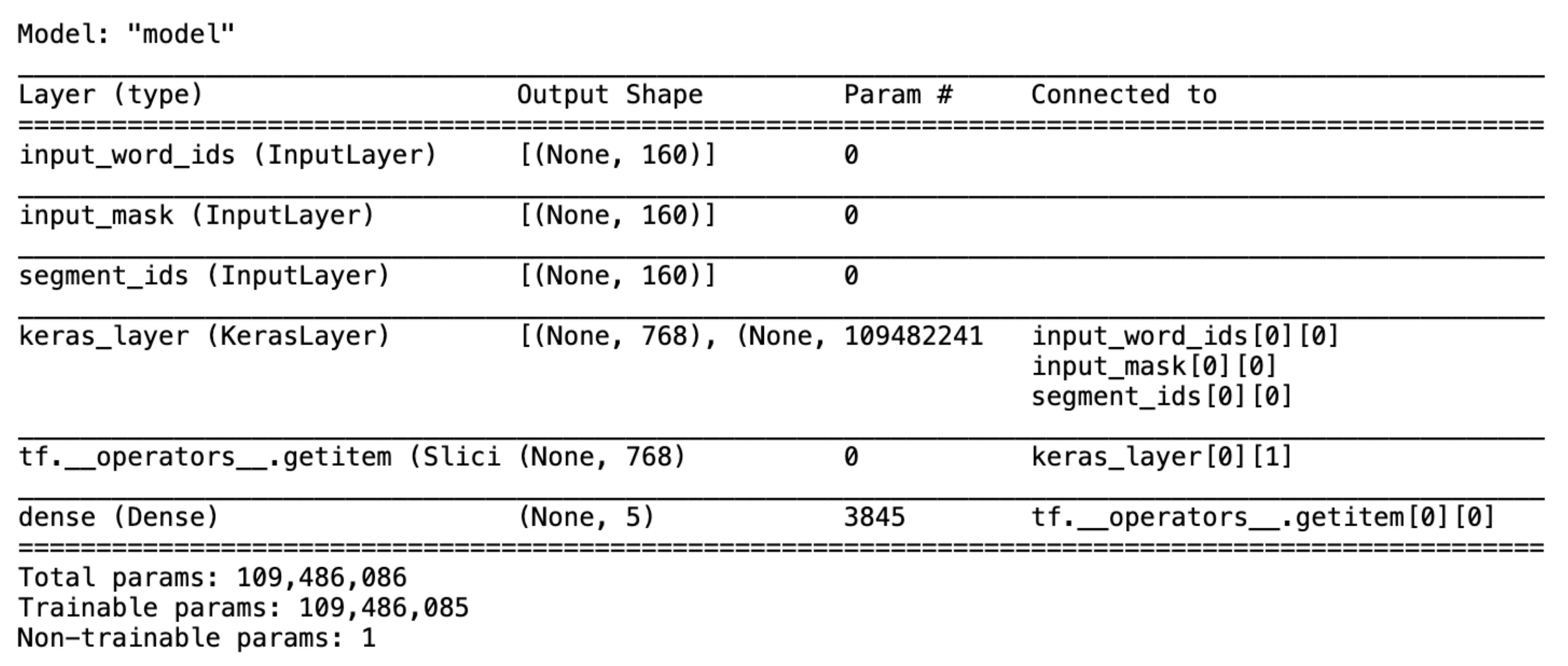
We now focus on the deep learning models. The LSTM model obtained an accuracy and an F1-score of 67%. In other words, LSTM provided slightly better results than MLP and significantly overcame the traditional machine learning classifiers. Finally, BERT achieved the best results, reaching an accuracy and an F1-score of 71%. BERT obtained improvements of 16% in accuracy and 15% in the F1-score over Logistic Regression, the best of the traditional machine learning models. BERT’s scores were also significantly better than those obtained by the MLP, with a difference of 6 points above the accuracy of MLP (65%). When comparing the deep learning methods, it can be said that BERT showed an improvement of 4 points in terms of accuracy and F1-score.
Table 3 shows the classification scores of the logistic model divided by the sentiment classes. Both the negative and the positive class were the ones with the lowest F1-scores, with 45% and 53%, respectively. These instances might have been wrongly classified in the extremely negative or positive categories, since they could be difficult to distinguish.
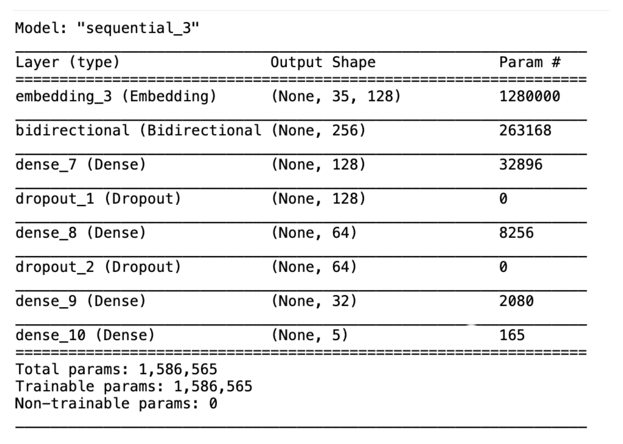
LSTM has a similar behaviour (see Table 4), but the classes with the lowest performance were the negative and the extremely negative classes. A large increase in the neutral class was seen, and the positive class remained similar to the negative class in terms of F1-score.
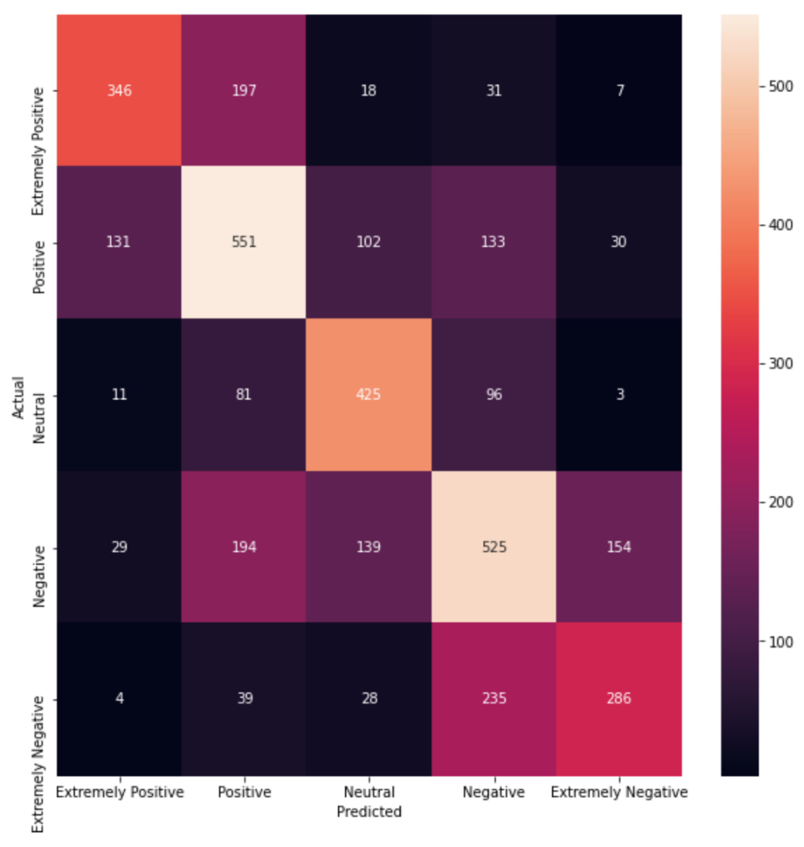
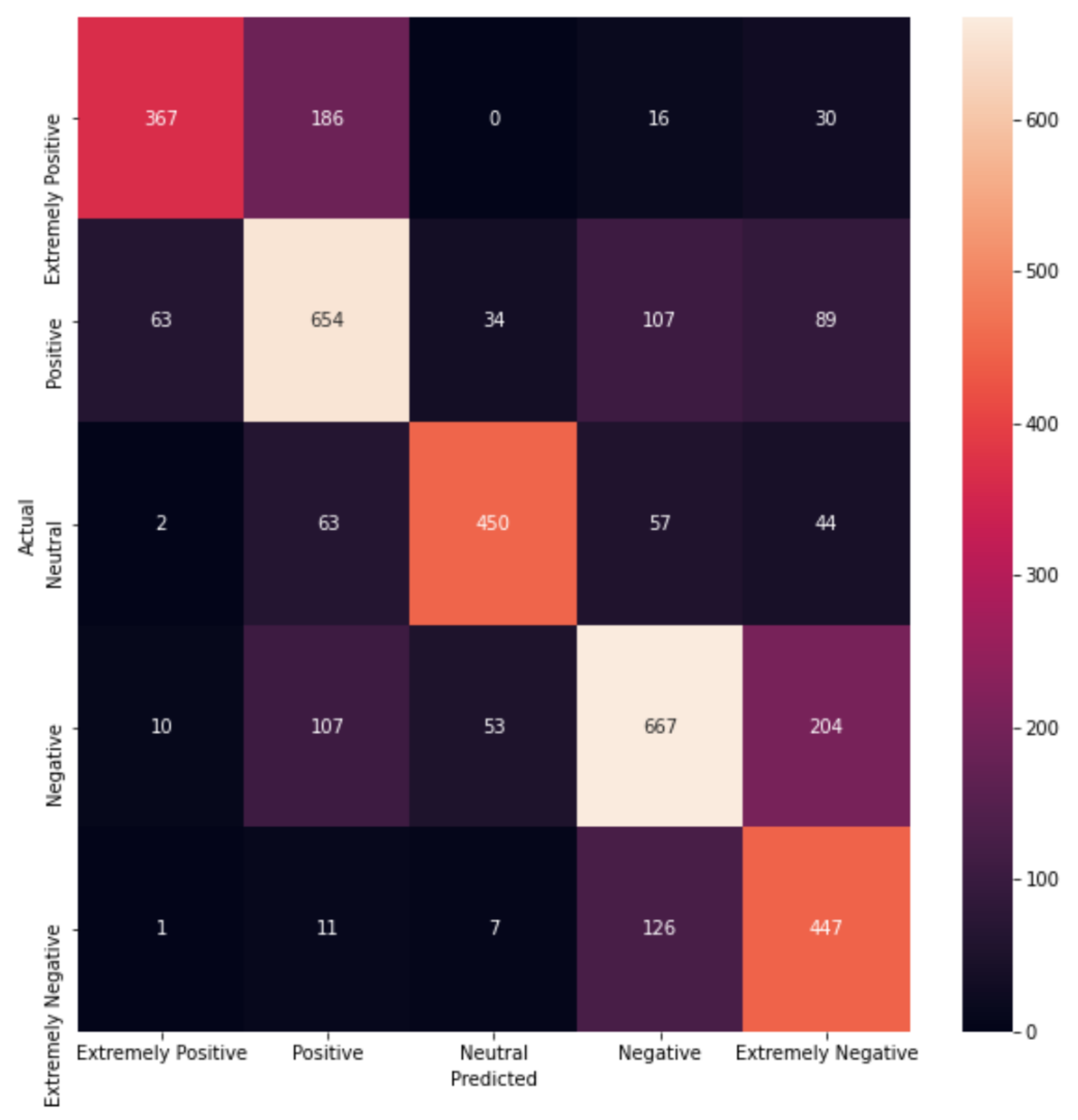
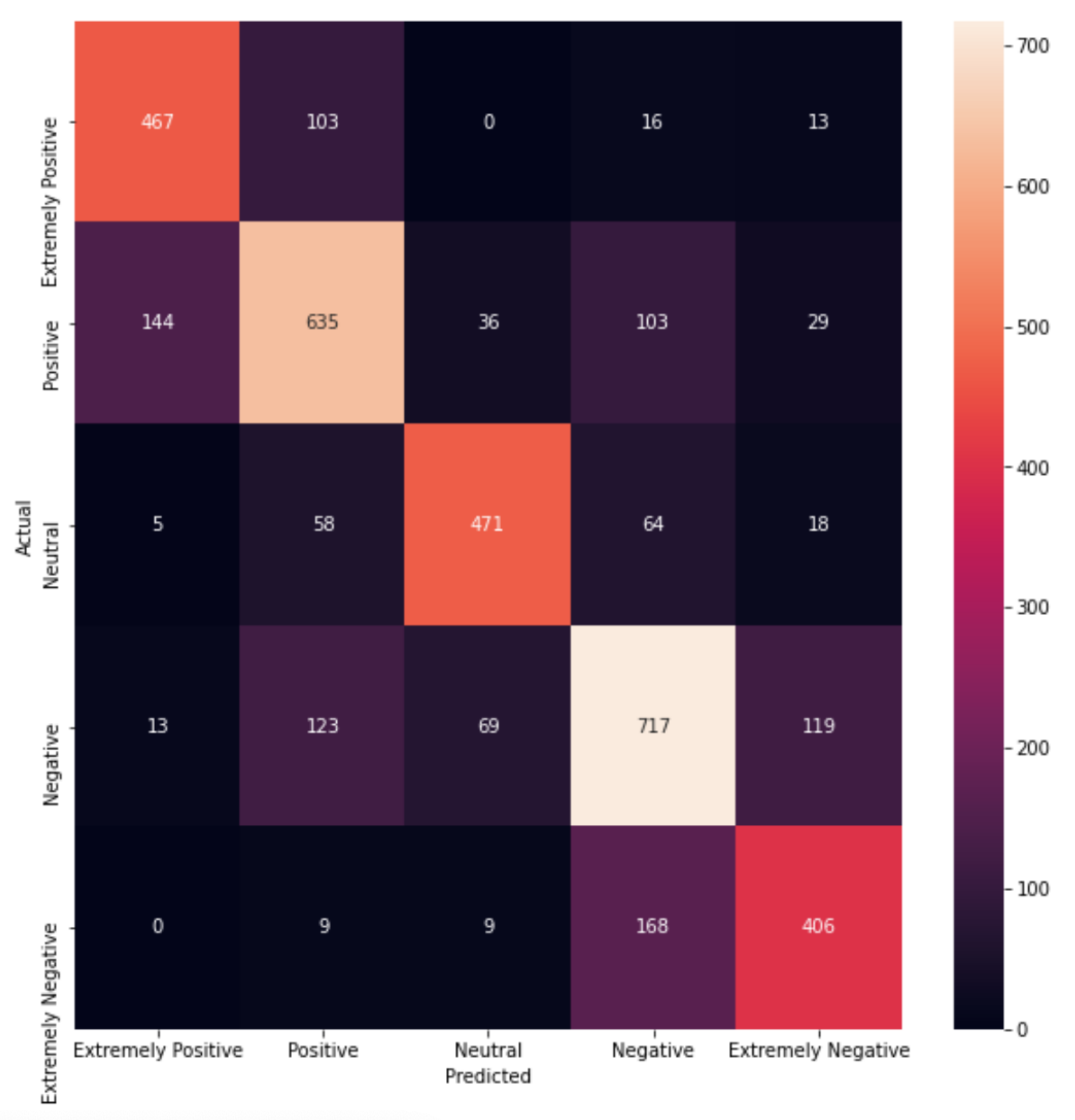
Table 5 shows a more detailed evaluation for the BERT model, providing scores for each class. It can be seen that the precision scores for the negative and the extremely negative classes were much lower than those of the positive or the neutral ones. In terms of the F1-score, the worst-performing classes were the positive and the negative, with a value of 68% each. Compared to the neutral class, this was very poor, since the neutral class had an F1-score of 78%, ten points higher. Overall, the accuracy of the model was 71%, which, at first glance, does not appear particularly high, but dealing with multiple classes is not as simple as the binary classification problem, where the benchmark is at 50%. As mentioned before, in this study, having five categories, a dummy classifier would obtain a 20% accuracy score. Therefore, achieving more than 70% shows very good performance indeed.
Finally, we can conclude that BERT showed its clear superiority in this task and was clearly the most accurate model to use in this sentiment classification task.
All the previous systems [21,22,23] trained on the same Kaggle dataset [3] only addressed the task of classifying negative, neutral and positive messages. In other words, they merged the instances from the extremely negative and negative classes, and they did the same for the extremely positive and positive classes. Therefore, a direct comparison to these systems’ models cannot be done. Similarly, the study presented in [24] only detected negative, neutral and positive tweets, obtaining a very high F1-score (around 98%). However, its results cannot be directly compared to ours, because we performed a finer-grained sentiment analysis of tweets about the COVID-19 pandemic.

3.3. Confusion Matrices

Confusion matrices are an excellent visual tool that allow the observer to distinguish the classes in which a model performs better [25]. Figure 7 shows the confusion matrix created with the predictions provided by the Logistic Regression model. In this case, we can see that the model was not very accurate, especially on the negative side, as there was much more distortion in this part of the model. It could also be noted that the neutral class might have been the most complicated class to choose. The main diagonal around this class was more disperse, as values predicted as neutral might actually have been negative or positive, or vice versa. In fact, this is a very difficult problem, even for humans, since, sometimes, correctly labelling a tweet as neutral or not might be a very challenging task. It is also very subjective, and since the tweets were all annotated by different people, their different perceptions might have affected the results.
The confusion matrices for the rest of the classical machine learning algorithms can be easily obtained by using the notebooks https://github.com/Joseantonio-96/Sentiment_Analysis (accessed on 3 November 2021).
Continuing with the analysis of the results, the confusion matrices of the LSTM and BERT models are presented in Figure 8 and Figure 9, respectively. It is easy to see the differences in these matrices compared to the matrix in Figure 7. The main diagonals are much more highlighted than in the matrix of Logistic Regression, meaning that the predicted categories of the instances matched their actual values with greater frequency.
The main issue in the predictions of these two models was no longer the neutral class, but the difference between the extremely positive or extremely negative with the positive and the negative classes, respectively. The reader might note that there is a connection between the misclassified observations in the four categories. Although the BERT model improved the precision of the positive polarities, the negative polarities still remained an issue. In fact, the difference between the extremely negative and negative class might be very different coming from two distinct persons, since it is a very subjective borderline.

3.4. Performance of the Models

The computational complexity of the models is also a topic of great interest, since, when dealing with very large datasets, we should keep in mind the time that the model will spend training and then predicting each instance. If the model is to be used in daily applications, it must be agile as well as accurate. We now discuss the training time of each model.
Table 6 below shows the training times of each model. It can be seen that, in general, the classical machine learning models would take only a few seconds to train. For the deep learning models, MLP was the fastest, taking only 2.3 min to train and reaching a convergence in only seven epochs.
Another observation that is worth discussing is the great difference in time elapsed from the LSTM and the BERT models; the former took only 8.25 min to converge, while the latter took 196.25 min. Although the F1-score of the BERT model was 72%, which is higher than that of the LSTM model by almost a 6% difference, the elapsed time to train this model was almost 25 times higher. This must be considered when choosing the best model, but it will obviously depend on the kind of application in which it will be used. The model with the highest accuracy/time ratio was MLP.

3.5. Convergence of the Deep Learning Models

Deep learning models are trained in epochs. An epoch refers to when all the data from the training set are passed through the model [26]. This is usually done in batches of a fixed amount of instances. It must be noted that, normally, a model can learn and achieve better validation accuracy scores by training in every new epoch. However, overfitting must also be considered, as more epochs do not necessarily mean better results. To this end, a percentage of the training set was used as the validation dataset.
Figure 10, Figure 11 and Figure 12 show that the training and validation loss and accuracy scores converge as the model trains through more epochs. It is interesting to note that both the MLP and LSTM model needed very few epochs to converge, 6 and 5, respectively. In particular, in MLP, we see a divergence of the training and validation very early on.
The BERT model, on the contrary, trains for 12 epochs until the validation and the training scores start to diverge, and early stopping is applied to avoid overfitting.
As an example, some of the predictions given by the model are presented in Table 7. It can be seen that, in most cases, the model accurately matches the actual sentiment of the tweet. The two first rows contain a positive and an extremely positive example, which were correctly classified. In both these examples, words such as “sweet”, “best” and “nice” were used, which might have made the decision easier. However, in the case of the fourth example, where the model classified the tweet as being negative but it was actually labelled as positive, the tweet did not contain any specific words with positive or negative polarity, and therefore was much more difficult to classify.

4. Conclusions

The spread of messages through social media platforms, particularly Twitter, during the COVID-19 pandemic has had a significant impact on almost every user of the platform. Of course, the messages have infinite implications, with some of them being positive, others negative and others being completely neutral. The use of NLP can have a positive impact by identifying and preventing the spread of erroneous, alarmist and hateful messages. Moreover, depression or anxiety problems could be prevented, and some solutions might be implemented to tackle these problems early on, by not allowing them to become out of control.
This study has explored several algorithms for the multi-class classification of tweets related to the COVID-19 pandemic.
The best model was the BERT model, achieving a macro F1-score of 71%, followed by the LSTM model, with an overall macro F1-score of 67%. The deep learning models clearly outperformed the traditional machine learning models.
Future works should be performed by including contextual information such as the date and location of the tweet. These two aspects could give relevant information and more conclusions could be made regarding certain dates and geographical locations around the world.
We also plan to explore other pre-trained language models such as RoBERTa (Robustly Optimized BERT Pretraining Approach) OpenAI’s GPT-3, ALBERT or XLNet [27].

Author Contributions

Methodology, J.A.J.-V. and I.S.-B.; software, J.A.J.-V.; validation, J.A.J.-V.; formal analysis, J.A.J.-V. and I.S.-B.; investigation, J.A.J.-V. and I.S.-B.; writing J.A.J.-V. and I.S.-B.; supervision, I.S.-B. All authors have read and agreed to the published version of the manuscript.

Funding

This work has been supported by the Madrid Government (Comunidad de Madrid) under the Multiannual Agreement with UC3M in the context of “Fostering Young Doctors Research” (NLP4RARE-CM-UC3M), as well as in the context of “Excellence of University Professors” (EPUC3M17) and in the context of the V PRICIT (Regional Programme of Research and Technological Innovation).

Institutional Review Board Statement

Not applicable.

Informed Consent Statement

Not applicable.

Data Availability Statement

All code used for this study can be found in the following Github repository: https://github.com/Joseantonio-96/Sentiment_Analysis (accessed on 3 November 2021). As for the data used, they can be found at the following Kaggle competition website https://www.kaggle.com/c/sentiment-analysis-of-covid-19-related-tweets/overview/description (accessed on 3 November 2021).

Conflicts of Interest

The authors declare no conflict of interest.

Abbreviations

The following abbreviations are used in this manuscript:
NLPNatural language Processing
MLMachine Learning
DLDeep Learning
SVMSupport Vector Machine
LSTMLong Short-Term Memory
BERTBidirectional Encoder Representation for Transformers

References

  1. González-Padilla, D.A.; Tortolero-Blanco, L. Social media influence in the COVID-19 pandemic. Int. Braz. J. Urol. 2020, 46, 120–124. [Google Scholar] [CrossRef] [PubMed]
  2. Losada, D.E.; Crestani, F.; Parapar, J. Overview of erisk 2018: Early risk prediction on the internet (extended lab overview). In Proceedings of the 9th International Conference of the CLEF Association, CLEF, Avignon, France, 10–14 September 2018; pp. 1–20. [Google Scholar]
  3. Coronavirus Tweets NLP-Text Classification. Available online: https://www.kaggle.com/c/sentiment-analysis-of-covid-19-related-tweets/overview/description (accessed on 25 March 2021).
  4. Hochreiter, S.; Schmidhuber, J. Long short-term memory. Neural Comput. 1997, 9, 1735–1780. [Google Scholar] [CrossRef] [PubMed]
  5. Devlin, J.; Chang, M.; Lee, K.; Toutanova, K. BERT: Pre-training of Deep Bidirectional Transformers for Language Understanding. In Proceedings of the 2019 Conference of the North American Chapter of the Association for Computational Linguistics: Human Language Technologies, NAACL-HLT 2019, Minneapolis, MN, USA, 2–7 June 2019; Volume 1 (Long and Short Papers). Burstein, J., Doran, C., Solorio, T., Eds.; Association for Computational Linguistics: Minneapolis, MN, USA, 2019; pp. 4171–4186. [Google Scholar] [CrossRef]
  6. Pedregosa, F.; Varoquaux, G.; Gramfort, A.; Michel, V.; Thirion, B.; Grisel, O.; Blondel, M.; Prettenhofer, P.; Weiss, R.; Dubourg, V.; et al. Scikit-learn: Machine Learning in Python. J. Mach. Learn. Res. 2011, 12, 2825–2830. [Google Scholar]
  7. Bergstra, J.; Bardenet, R.; Bengio, Y.; Kégl, B. Algorithms for hyper-parameter optimization. In Proceedings of the 25th Annual Conference on Neural Information Processing Systems (NIPS 2011), Neural Information Processing Systems Foundation, Granada, Spain, 12–15 December 2011; Volume 24. [Google Scholar]
  8. Bergstra, J.; Yamins, D.; Cox, D. Making a science of model search: Hyperparameter optimization in hundreds of dimensions for vision architectures. Int. Conf. Mach. Learn. PMLR 2013, 28, 115–123. [Google Scholar]
  9. Leung, H.; Haykin, S. The complex backpropagation algorithm. IEEE Trans. Signal Process. 1991, 39, 2101–2104. [Google Scholar] [CrossRef]
  10. Ramchoun, H.; Idrissi, M.A.J.; Ghanou, Y.; Ettaouil, M. Multilayer Perceptron: Architecture Optimization and Training. Int. J. Interact. Multim. Artif. Intell. 2016, 4, 26–30. [Google Scholar] [CrossRef]
  11. Wang, Y.; Huang, M.; Zhu, X.; Zhao, L. Attention-based LSTM for aspect-level sentiment classification. In Proceedings of the 2016 Conference on Empirical Methods in Natural Language Processing, Austin, TX, USA, 1–5 November 2016; pp. 606–615. [Google Scholar]
  12. Sherstinsky, A. Fundamentals of recurrent neural network (RNN) and long short-term memory (LSTM) network. Phys. D Nonlinear Phenom. 2020, 404, 132306. [Google Scholar]
  13. Sundermeyer, M.; Schlüter, R.; Ney, H. LSTM neural networks for language modeling. In Proceedings of the Thirteenth Annual Conference of the International Speech Communication Association, Portland, OR, USA, 9–13 September 2012. [Google Scholar]
  14. Bisong, E. Google colaboratory. In Building Machine Learning and Deep Learning Models on Google Cloud Platform; Springer: Berlin/Heidelberg, Germany, 2019; pp. 59–64. [Google Scholar]
  15. Brownlee, J. Deep Learning with Python: Develop Deep Learning Models on Theano and TensorFlow Using Keras; Machine Learning Mastery. 2016. Available online: https://core.ac.uk/download/pdf/41172947.pdf (accessed on 3 November 2021).
  16. Hossin, M.; Sulaiman, M. A review on evaluation metrics for data classification evaluations. Int. J. Data Min. Knowl. Manag. Process 2015, 5, 1. [Google Scholar]
  17. Menardi, G.; Torelli, N. Training and assessing classification rules with imbalanced data. Data Min. Knowl. Discov. 2014, 28, 92–122. [Google Scholar] [CrossRef]
  18. Forman, G. An extensive empirical study of feature selection metrics for text classification. J. Mach. Learn. Res. 2003, 3, 1289–1305. [Google Scholar]
  19. El Alaoui, I.; Gahi, Y.; Messoussi, R. Big data quality metrics for sentiment analysis approaches. In Proceedings of the 2019 International Conference on Big Data Engineering, Hong Kong, China, 11–13 June 2019; pp. 36–43. [Google Scholar]
  20. Tyagi, A.; Sharma, N. Sentiment analysis using logistic regression and effective word score heuristic. Int. J. Eng. Technol. (UAE) 2018, 7, 20–23. [Google Scholar] [CrossRef]
  21. Tokenization in NLP. Available online: https://www.kaggle.com/satishgunjal/tokenization-in-nlp (accessed on 20 May 2021).
  22. Birla, V. [Transformers] COVID-19 Tweets Sentiment Analysis. Available online: https://www.kaggle.com/immvab/transformers-covid-19-tweets-sentiment-analysis (accessed on 21 May 2021).
  23. Anubhavsanyal. Tensorflow with LSTM- 83% Accuracy. Available online: https://www.kaggle.com/anubhavsanyal/tensorflow-with-lstm-83-accuracy/notebook (accessed on 20 May 2021).
  24. Satu, M.S.; Khan, M.I.; Mahmud, M.; Uddin, S.; Summers, M.A.; Quinn, J.M.; Moni, M.A. Tclustvid: A novel machine learning classification model to investigate topics and sentiment in covid-19 tweets. Knowl.-Based Syst. 2021, 226, 107126. [Google Scholar] [CrossRef] [PubMed]
  25. Loomis, J.M. Analysis of tactile and visual confusion matrices. Percept. Psychophys. 1982, 31, 41–52. [Google Scholar] [CrossRef] [PubMed]
  26. Osawa, K.; Tsuji, Y.; Ueno, Y.; Naruse, A.; Yokota, R.; Matsuoka, S. Second-order optimization method for large mini-batch: Training resnet-50 on imagenet in 35 epochs. arXiv 2018, arXiv:1811.12019. [Google Scholar]
  27. Yang, Z.; Dai, Z.; Yang, Y.; Carbonell, J.; Salakhutdinov, R.R.; Lee, Q.V. XLNet: Generalized Autoregressive Pretraining for Language Understanding. In Proceedings of the Advances in Neural Information Processing Systems, Vancouver, BC, Canada, 8–14 December 2019. [Google Scholar]
Figure 1. Class distribution of the training dataset.
Information 12 00459 g001
Figure 2. Class distribution of the test dataset.
Information 12 00459 g002
Figure 3. Hyperparameters of MLP.
Information 12 00459 g003
Figure 4. Architecture of our LSTM model.
Information 12 00459 g004
Figure 5. Architecture of our BERT model.
Information 12 00459 g005
Figure 6. Binary classification confusion matrix.
Information 12 00459 g006
Figure 7. Confusion matrix for the logistic model predictions.
Information 12 00459 g007
Figure 8. LSTM model.
Information 12 00459 g008
Figure 9. BERT model.
Information 12 00459 g009
Figure 10. MLP—loss and accuracy convergence.
Information 12 00459 g010
Figure 11. LSTM—loss and accuracy convergence.
Information 12 00459 g011
Figure 12. BERT—loss and accuracy convergence.
Information 12 00459 g012
Table 1. Hyperparameters selected per model.
ModelHyperParametersHPO Method
SVN{C = 1, kernel = ‘rbf’, tol = 1 × 10 3 and gamma = ’scale’}Randomised Search
Logistic Regression{ C = 25, penalty = ‘l2’, tol = 1 × 10 4 , solver = ’lbfgs}Grid Search
Gaussian Naive Bayes{proirs = 5, var_smoothing = 1 × 10 9 }Randomised Search
Multinomial Naive Bayes{alpha = 1, fit_prior = True, fit_classes = 5}Randomised Search
Random Forest{min_samples_split: 100, min_samples_leaf: 2, max_depth: 256}Randomised Search
Table 2. Macro-averaged resulsts for each model. Best scores are in bold.
ModelPrecisionRecallF1Accuracy
Gaussian Naive Bayes0.360.420.320.35
Multinomial Naive Bayes0.520.420.430.45
Random Forest0.490.470.470.47
Support Vector Machine0.540.550.550.53
Logistic Regression Model0.560.570.560.55
Multilayer Perceptron0.660.660.660.65
LSTM0.680.670.670.67
BERT0.720.720.710.71
Table 3. Results per class obtained by the logistic model.
ClassPrecisionRecallF1-ScoreSupport
Extremely Negative0.560.560.56592
Negative0.500.410.451041
Neutral0.590.690.64616
Positive0.500.560.53947
Extremely Positive0.660.630.64599
Table 4. Results per class of the LSTM model.
ClassPrecisionRecallF1-ScoreSupport
Extremely Negative0.550.720.62592
Negative0.660.600.631041
Neutral0.800.720.76616
Positive0.620.680.65947
Extremely Positive0.790.630.70599
Table 5. Evaluation scores per class for the BERT model.
ClassPrecisionRecallF1-ScoreSupport
Extremely Negative0.660.760.71592
Negative0.670.680.681041
Neutral0.810.760.78616
Positive0.690.670.68947
Extremely Positive0.790.730.76599
Table 6. Training times per model.
ModelTime Elapsed (min.)
Support Vector Machine0.05
Logit Model2.5
Gaussian Naive Bayes0.04
Multinomial Naive Bayes0.025
Random Forest4.3
NN-MLP2.3
NN-LSTM8.25
NN-BERT196.91
Table 7. Example tweets with actual and predicted sentiment class.
TweetActual SentimentPredicted Sentiment
If you re considered at risk during the outbreak now is the time to stock up on supplies including food medicine amp cleaning supplies Be sure you have over the counter medicines amp medical supplies to treat fever amp other symptoms.PositivePositive
best thing right spread compassion stressed anxious effort nice grocery store clerk reach friend online compliment stranger outfit wash handExtremely PositiveExtremely Positive
SkinCare: order grocery online standing q master link cooking grocery food household supply skincareNeutralNeutral
The parade of pharma, and other consumer issues is about the MARKET. Plain and simple. This sociopath does not care about us. #coronapocalypse #Covid19 parade pharma consumer issue market plain simple sociopath careNegativePositive
remember afford stock pile month food toilet paper sensitive live pay check pay checkNegativeNegative
Publisher’s Note: MDPI stays neutral with regard to jurisdictional claims in published maps and institutional affiliations.

