Predicting Stock Movements: Using Multiresolution Wavelet Reconstruction and Deep Learning in Neural Networks

Abstract

Stock movement prediction is important in the financial world because investors want to observe trends in stock prices before making investment decisions. However, given the non-linear non-stationary financial time series characteristics of stock prices, this remains an extremely challenging task. A wavelet is a mathematical function used to divide a given function or continuous-time signal into different scale components. Wavelet analysis has good time-frequency local characteristics and good zooming capability for non-stationary random signals. However, the application of the wavelet theory is generally limited to a small scale. The neural networks method is a powerful tool to deal with large-scale problems. Therefore, the combination of neural networks and wavelet analysis becomes more applicable for stock behavior prediction. To rebuild the signals in multiple scales, and filter the measurement noise, a forecasting model based on a stock price time series was provided, employing multiresolution analysis (MRA). Then, the deep learning in the neural network method was used to train and test the empirical data. To explain the fundamental concepts, a conceptual analysis of similar algorithms was performed. The data set for the experiment was chosen to capture a wide range of stock movements from 1 January 2009 to 31 December 2017. Comparison analyses between the algorithms and industries were conducted to show that the method is stable and reliable. This study focused on medium-term stock predictions to predict future stock behavior over 11 days of horizons. Our test results showed a 75% hit rate, on average, for all industries, in terms of US stocks on FORTUNE Global 500. We confirmed the effectiveness of our model and method based on the findings of the empirical research. This study’s primary contribution is to demonstrate the reconstruction model of the stock time series and to perform recurrent neural networks using the deep learning method. Our findings fill an academic research gap, by demonstrating that deep learning can be used to predict stock movement.

1. Introduction

In the financial world, stock price forecasting is crucial [1,2,3,4]. The purpose of stock price prediction is optimizing stock investments. However, due to the high volatility of stock prices, it is difficult to investigate the uncertainty of factors, such as time series [5,6], which affect the stock price behavior [7]. As a result, predicting stock price movement accurately is a necessary, but difficult, task.

In the past decades, to improve the predictability of the results, research has been conducted. However, dealing with non-linear, non-stationary, and large-scale financial time series features remains a difficult task, as it is difficult to illustrate the stock market’s features comprehensively. Because the stock market is an inherently volatile, complex, and highly non-linear system [8], and it is affected by policies and many other factors, it cannot be easily measured or calculated. Thus, researchers focusing on this area continuously seek to improve the accuracy of these predictions by developing more advanced tools and methods [3]. As a useful time-frequency analysis tool, wavelet analysis has good localized properties. This tool is especially suitable for multi-scale analysis because it can reflect the change of the instantaneous frequency structure in the time series with multi-level and multiresolution advantages. With this tool, the stock market data can be decomposed into multi-scale time series data via wavelet multiresolution [9]. Following this, the stock market time series information is extracted at different scales.

Deep learning is a rapid growth machine learning method. It is attractive to researchers and traders not only because it can deal with a massive amount of historical data, but also because it can find hidden non-linear rules. It creates a better feature space by utilizing multiple layers [10]. However, there is insufficient research to support the claim that deep learning is a suitable tool for stock price prediction.

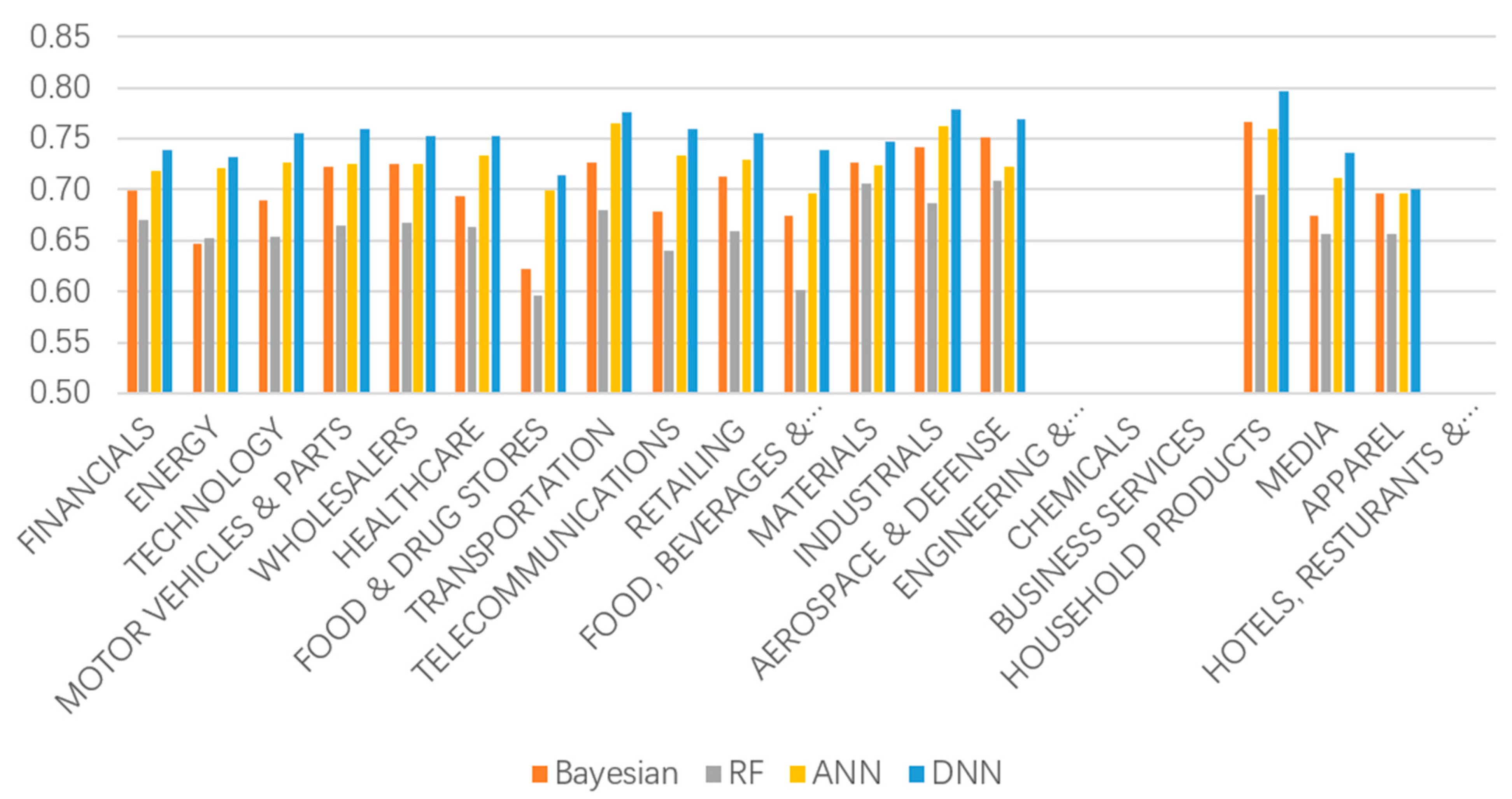
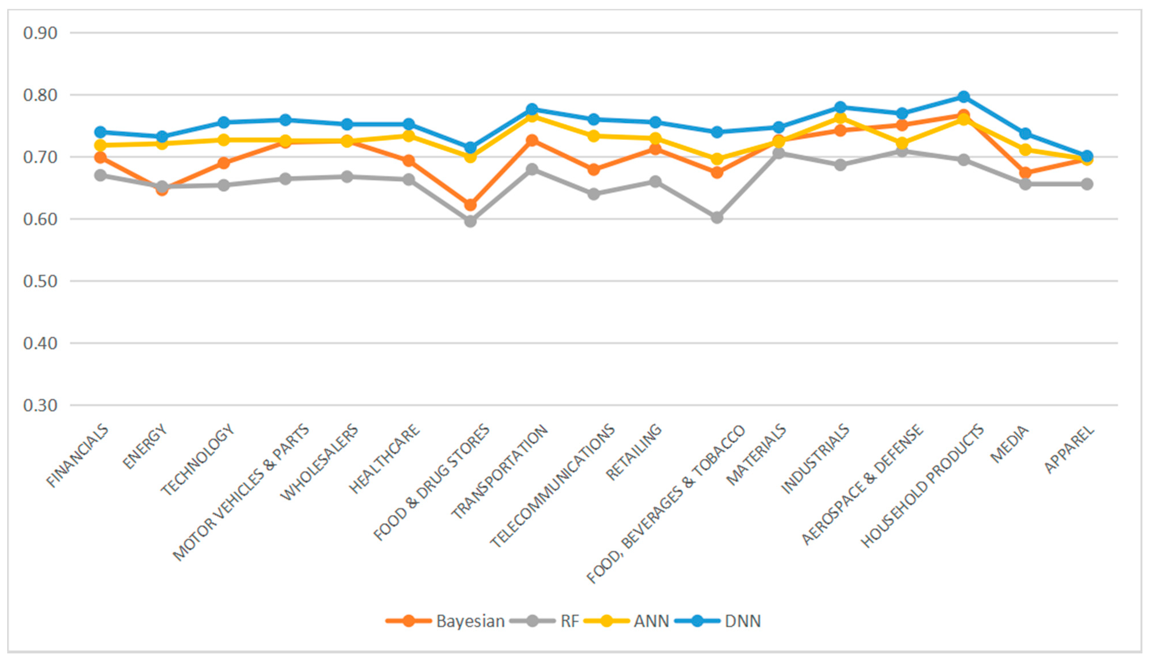
The primary contribution of this study is to demonstrate the reconstruction model of the stock time series and to perform recurrent neural networks by using the deep learning method. In particular, firstly, the number of instances (transaction dates) and the number of sample stocks we used is bigger. We selected the stock price data ranging from 1 January 2009 to 31 December 2017; the data set of which is big enough to capture a high diversity in price movements. We studied a more substantial number of stocks and tested the behavior of each of the 168 stocks to learn more instances. Secondly, we focus on medium-term stock predictions to predict future stock behavior over 11 days of horizons. Because trades do not have to happen within milliseconds, but can be liquid, and open and close in a trading day, mid-term predictions are more helpful for the long-term decisions. Thirdly, we found that the deep learning method works more stably and reliably than the traditional machine learning methods. Lastly, we stand on the industry view to do the comparison analysis. In most industries, the DNN prediction results are higher than 75%. Among these, the mean result of DNN for the financial industry, energy industry, and technology industry, which have a large sample of stocks, is roughly around 75%. The empirical results show that the practical result of our algorithm is higher than 75%. We observed that by using our model, the household products industry gets the highest accuracy result, and the apparel industry gets the lowest. One explanation is that these two industries do not have a sufficient number of stocks in this sample, so one single stock will have a significant impact on the industry average.

Historically, the DNNs method has been used infrequently in conjunction with wavelet analysis to forecast stock movement. Our research attempted to bridge the gap. The rest of the paper is organized as follows: First, in Section 2, we list some recent work related to our study. Section 3 describes our model and method using MRA. Section 4 describes our data set and assesses the results of the empirical tests. As the last section, Section 5 concludes our research and discusses future work.

2. Related Work

In this section, we review the relevant research, including stock price behavior prediction, wavelet analysis, deep learning, and neural networks. Based on the limitation of previous studies, our research model and solutions are proposed.

2.1. Predictability of Stock Price Movement

In the discussion of whether stock price behavior is predictable, investors and some researchers have accepted the efficient market hypothesis (EMH) [11]. The EMH states that the past behavior of stock prices can be studied to reflect both current and future information to predict unpredictable stock prices [12,13]. For stock predictions, a level of directional accuracy, with a 56% hit rate, is often recognized as a satisfying result [14,15]. Therefore, multiple methods and algorithms have been shown to explain how the stock price behavior can be forecasted, and how to improve the forecast results.

There are several types of prediction. Past attempts can be classified into three categories, namely, technical analysis, fundamental analysis, and traditional time series forecasting [16,17]. Professional traders and researchers tried to use more-advanced techniques to get more-precise results. Therefore, to make it simple, the primary methods for stock price prediction can be classified into two categories—technical analysis and fundamental analysis [18]. Fundamental analysis studies a company’s operations, economic indicators, and financial conditions to predict future stock price. Contrarily, technical analysis uses a stock’s historical price as a reference to predict the future price [12]. This approach covers technical methods, from traditional statistical methods, such as the autoregressive-moving average model, to the new artificial intelligence (AI) [19]. Machine learning methods are primarily used nowadays [1]. Our research uses different algorithms as part of the technical methods.

Stock movement prediction is useful for both short-term and long-term forecasting. Some studies make short-term-oriented predictions. They predict the immediate stock price reaction following the measure of stock prices between minutes and the end of the trading day [20]. Trades do not have to happen within milliseconds, but can be liquid, and open and close in a trading day. Therefore, in this paper, we focus on medium-term stock predictions. Based on the historical data of up to 10 days of the past, we predict future stock behavior over 11 days of horizons.

2.2. Multiresolution Reconstruction Using Wavelets

As an effective time-frequency analysis tool, wavelet analysis has good localized properties in the time and frequency domains. This tool is especially suitable for multi-scale analysis because it can reflect the change of the instantaneous frequency structure in the time series, with localized and multiresolution advantages. Our study presents a forecasting model based on the stock price time series, using multiresolution analysis (MRA) to reconstruct the signals in multiple scales and filter the measurement noise. We first decomposed the stock market data into multi-scale time series data, which can be referred to as multiresolution analysis using wavelet, and then extracted the results to output. Based on long memory stochastic volatility (LMSV), the autocorrelation analysis and the cross-correlation analysis are proposed. The autocorrelation shows the dynamic and memory features of the series, and also shows the memory length of the time series data. Cross-correlation analysis can find out the coupling between two scales of data. Based on the strength of the coupling, we can determine the trade-offs of data. In our research, we study the stock market behavior from a multi-scale perspective, using wavelet. Then, we use deep neural networks to train and test the empirical data set. With the accuracy results of testing the data, we conclude our method efficiently and effectively.

In the process of multi-scale feature extraction, the wavelet basis function is chosen according to the shape of the stock market timing data. That is because of the matching degree of wavelet basis function, together with the shape of the signal to be decomposed, which could directly affect the result of the multiresolution analysis. The number of decomposition scales is determined according to the step size and the length of experimental data. In our study, the wavelet coefficients and the related scale coefficients are reduced by 2 m, where m is the scale of the decomposition [21].

2.3. Neural Networks

The artificial neural networks (ANNs, the conventional neural networks) algorithm is one of the artificial intelligence methods that has been developed and used to predict stock price movement [22,23,24,25,26,27,28]. White first used neural networks in stock market prediction [29].

Table 1. Research relates to stock price prediction using neural networks.

Authors (Year)	Method	Sample Period	Forecast Type	Accuracy
Wuthrich et al. (1998) [30]	ANNs, rule-based	6-Dec-1997 to 6-Mar-1998 (daily)	Market direction (up, steady or down)	43.6%
Groth and Muntermann (2011) [31]	ANNs	1-Aug-2003 to 31-Jul-2005 (daily)	Trading signal (stock price)	-
Enke and Mehdiyev (2013) [32]	Fuzzy NNs, fuzzy clustering	Jan-1980 to Jan-2010 (daily)	Stock price	-
Chiang, Enke, Wu, and Wang (2016) [33]	ANNs, particle swarm optimization	Jan-2008 to Dec-2010 (daily)	Trading signal (stock price)	-
Arevalo, Nino, Hernandez, and Sandoval (2016) [34]	DNNs	2-Sep-2008 to 7-Nov-2008 (1 min)	Stock price	66%
Zhong and Enke (2017) [35]	ANNs, dimension reduction	1-Jun-2003 to 31-May-2013 (daily)	Market direction (up or down)	58.1%
Singh and Srivastava (2017) [12]	DNNs, dimension reduction	19-Aug-2004 to 10-Dec-2015 (daily)	Stock price	-
(Lei, 2018) [7]	Wavelet NNs, rough set (RS)	2009 to 2014, five different stock markets	Stock price trend	65.62~66.75%
Our approach	Deep learning in RNNs, MRA	2013 to 2017, three different stock market, and S&P 500 stock index	Stock price movement

provides a summary of the recent research related to stock price prediction using neural networks.

Table 1 shows that the artificial neural network is widely used. The main reason is that artificial neural networks can learn to do multi-input parallel processing and can do non-linear mapping. However, in the application of conventional neural networks, the effect of the practical results is not ideal. There is no more effective theoretical guidance for the determination of the number of hidden layer neurons, the initialization of various parameters, or the neural network structure. So far, many improvements were made to make the algorithm more optimized. In recent years, deep artificial neural networks (including recurrent ones) have won numerous contests in machine learning.

2.4. Deep Learning

Deep learning is a set of methods that use deep architectures to learn high-level feature representations [36]. It builds an improved feature space by using multiple layers, emerged as a new area of machine learning research. Deep learning originated from image recognition, and has been extended to all areas of machine learning. Similarly to the traditional machine learning methods, deep learning can be trained to learn the relationship between features and tasks. However, in contrast to traditional methods, deep learning can automatically extract more-complex features from simple features. It uses the features of the last layer of abstraction to classify the training data. Figure 1 shows the difference between the deep learning process and the traditional machine learning process.

Deep neural networks (NNs) have also become useful when there is no supervision of learning. Among ANNs, both feedforward neural networks (FNNs) and recurrent (cyclic) neural networks (RNNs) have been used mainly in research. Recurrent neural networks (RNNs), in theory, can approximate arbitrary dynamical systems with arbitrary precision comparable to other traditional ANNs. However, RNNs are different from FNNs. FNN models adopt the backpropagation (BP) algorithm to adjust parameters. An efficient gradient descent method for teacher-based supervised learning in discrete networks is called backpropagation (BP), and was applied in NNs in 1981. However, the BP-based training of deep NNs had been found to be difficult in practice by the late 1980s. Contrarily, for RNNs, the BP algorithm is not used. If all layers are trained at the same time, the time complexity will be too high. If each layer is trained at one time, the deviation will be transmitted, and overfitting will occur. In a sense, RNNs are the deepest of all NNs, and can create and process memories of arbitrary sequences of input patterns [37].

Both RNN and FNN use a hierarchical structure, in the following way: a multi-layer network includes an input layer, hidden layer(s), and output layer. RNNs are cyclic and FNNs are acyclic graphs. Within the recurrent networks, each layer can be regarded as a logistic regression model. As is shown in Figure 2, there is no connection between the same-layer nodes or the cross-layer nodes; only the adjacent-layer nodes can be connected.

2.5. Wavelet and Deep Neural Networks

The concept of wavelet network architecture was explicitly set forth in 1992. The basic idea was to use waveron to replace neurons, with a rational approximation of wavelet decomposition to establish the link between wavelet transform and neural networks [38]. Then, an orthogonal-based wavelet neural network was proposed, by using a scaling function as the excitation function [39]. The orthogonal wavelet neural network and its learning algorithm are presented [40]. The basic idea is to analysis the data using wavelet decomposition. By multiresolution analysis (MRA), some excitation functions in hidden layers are using scaled functions, and some are using wavelet functions. Figure 3 shows a flowchart of our proposed idea. We first use wavelet decomposition as a de-noising of the time series data, and then we use the wavelet and scaling function as the excitation function of neurons.

Wavelet neural networks (WNN) are the combination of the following two theories: the wavelets and the neural networks. The wavelet-based neural network architecture is a new neural network based on wavelet analysis [7]. It has more theory foundations and good feature selection capabilities. Wavelet neural networks use one hidden layer and consist of a feedforward neural network. It takes one or more inputs, and the output layer that consists of one or more linear combiners. Wavelet analysis has good time-frequency local characteristics and good zooming capability for non-stationary random signals. The neural networks method is a powerful tool to deal with large-scale problems. Therefore, the combination of neural networks and wavelet analysis becomes more applicable for stock behavior prediction.

3. Multiresolution Wavelet Analysis and Correlation Analysis Model

In this section, we review the relevant research, including multi-scale analysis for the time series and correlation analysis of the time series. A model of multiresolution analysis is proposed for stock price prediction.

3.1. Multi-Scale Analysis for Time Series

The fast wavelet transform (FWT), which is based on orthogonal wavelet and MRA, can decompose signals into different components at different scales [41]. The realization process is similar to using a set of high-pass and low-pass filters step by step. The high-pass filter generates the high-frequency detail components, and the low-pass filter generates the low-frequency detail components of the signal. The bandwidth for the two components of the filter is equal. The next step is to repeat the above process for the low-frequency component, to obtain the two decomposed components of the next layer. This method can deal with signals such as the stock price fluctuating on a regular basis.

To describe the wavelet transform algorithm, we denote the time series x\left(t\right) of the original stock price series with the Formulas (1), (2), and (3), which explains the low-frequency signals and high-frequency signals.

$$x\left(t\right)={\sum }_k{s}_{J,K}{\omega }_{J,K}\left(t\right)+{\sum }_k{d}_{J,K}{\psi }_{J,K}\left(t\right)+{\sum }_k{d}_{J-1,K}{\psi }_{J,K}\left(t\right)+\cdots +{\sum }_k{d}_{1,K}{\psi }_{J,K}\left(t\right)$$

(1)

$$S_J\left(t\right)={\sum }_k{s}_{J,K}{\omega }_{J,K}\left(t\right)$$

(2)

$$D_J\left(t\right)={\sum }_k{d}_{J,K}{\psi }_{J,K}\left(t\right)$$

(3)

So, the original signal series could be expressed as the sum of each component, as follows:

$$x\left(t\right)={\sum }_{j=1}^J{D}_J\left(t\right)+S_J\left(t\right)$$

(4)

where j is the decomposition level, which ranges from 1 to J; k is the translation parameter; ${\omega }_{J,K}\left(t\right)$ and ${\psi }_{J,K}\left(t\right)$ are the parent wavelet pairs; $s_{J,K}$ is the scaling coefficient of the father wavelet ${\omega }_{J,K}\left(t\right)$; and $d_{J,K}$ is the detail coefficient of the mother wavelet ${\psi }_{the J,K}\left(t\right)$. The detail and scaling coefficients with the basis vector from the level J are linked with time t and scale $\left[2^{J-1}, 2^J\right]$. $D_J\left(t\right)$ is the high-frequency component signal. $S_J\left(t\right)$ is the low-frequency component signal. For the last equation, $D_J\left(t\right)$ is also the recomposed series; $S_J\left(t\right)$ is the residue.

3.2. Correlation Analysis of Time Series

The time-varying LMSV model can describe long and short memory characteristics at various points in time. Xu introduced the wavelet transform coefficient into the estimation of the time-varying LMSV model parameters [42]. Given this characteristic of the coefficient of the LMSV process, the self-correlation and cross-correlation analysis of the reconstructed time series is performed after wavelet decomposition reconstruction. The multi-scale coefficients obtained from the correlation analysis are tested by the Dickey–Fuller method (augmented Dickey–Fuller test, ADF). It is assumed that neither the autocorrelation or the cross-correlation of the wavelet coefficients will be affected by the boundary conditions. The autocorrelation could characterize the dynamic and memory characteristics of the time series data. The cross-correlation analysis could discover the coupling between two scale timing data. We can determine the multi-scale timing data trade-offs according to the strength of the coupling.

The autocorrelation analysis is performed on the scale coefficients $s_J$ from the multi-scale analysis. The wavelet coefficient is $d_j$ (j = 1, 2…J), $d_j$ could determine the memory length for each scale factor. We keep the scale coefficients whose memory length is greater than the predicted step size. Then, the remaining part will be removed. If the cross-correlation between a certain two scale coefficients is strong, then there is a strong coupling relationship between them. We will remove one of the scale coefficients, for the strong coupling relationship will hinder the reduction in the data dimension. In summary, the model we built and the process we followed for stock price movement prediction using wavelet and multiresolution analysis can be shown in Figure 4.

The purpose of this paper is to decompose stock market data into multi-scale time series data and extract stock market time series information at different scales. In Figure 4, this model displays the basic model of multi-scale analysis and correlation analysis, aiming to express the principle of the multi-scale analysis of the time series and the correlation analysis of the multi-scale time series. Because the multi-scale sequence correlation analysis method is different from the ordinary time series correlation analysis, autocorrelation indicates the dynamic characteristics and memory characteristics of the underlying mechanism of the system that generates the series, and autocorrelation analysis can get the memory length of the time series data. From the cross-correlation analysis, we can find the coupling between the time series data of two scales, and judge the choice of multi-scale time series data according to the strength of the coupling. As a result, Section 3 explains how we divide sequences and conduct correlation analysis in this study.

4. Empirical Study

4.1. Data Collection

Our market data include New York Stock Exchange (NYSE), American Stock Exchange (AMSE), and NASDAQ. We chose stock price data from the US stock market between 1 January 2009 and 31 December 2017. Considering that a period that is extended enough can help to capture a high diversity in price movements and also avoid data snooping, we divide the data set into the following two parts: training and testing. The training set contains data from 1 January 2009 to 30 June 2017, and the testing set contains data from 1 July 2017 to 31 December 2017. The center for research in security prices (CRSP) is the primary database we used to export data for the stocks and market index. We define the data set that extracted from the multi-scale time series as the condition attribute set. The decision attribution set will be the future condition of the arithmetic average price after k days. On a daily basis, we chose the closing price (PRC), opening price (OPENPRC), ask or high price (ASKHI), bid or low price (BIDLO), and volume amount (VOL) as the decision attribution set.

Among the decision attribution set, we chose PRC as the judging criteria. That is, the decision set will be marked as one if PRC for the i + k day is lower than that of the ith day. Otherwise, the decision set will be marked as two. We do these to construct a decision table, which supports the classification prediction.

The predicted evaluation criteria are calculated using the following formula:

$$P=\frac{1}{m}{\sum }_{i=1}^m{D}_i \left(i=1,2,\cdots ,m\right)$$

(5)

In this formula, $D_i$ is defined as the prediction rising or falling value for the ith trading day, as follows:

$$D_i=\{\begin{array}{ll}1,& if P{O}_i=A{O}_i\\ 0, & otherwise\end{array}$$

(6)

where $P{O}_i$ is the predicted value for the ith trading day, and $A{O}_i$ is the actual value for the ith trading day, and m is the number of testing samples.

We selected a sample of publicly listed companies from FORTUNE Global 500 (FT Global 500), which is ranked by revenues in the year of 2017. We chose public companies listed in the US stock market as our sample set. Within the 500 global ranking companies in the year of 2017, there are 312 publicly listed companies worldwide, but only 168 companies listed in the US stock market. Therefore, we ran through each of the 168 companies to make the conclusion more convincing. Furthermore, FT Global 500 contributes a detail classification for industries. The industries and the number of companies are shown in

Table 2. Industries and the number of companies per industry.

Stock Industries	%
Financials	23.74
Energy	16.10
Technology	8.85
Motor Vehicles and Parts	6.84
Wholesalers	5.63
Healthcare	5.43
Food and Drug Stores	4.02
Transportation	3.82
Telecommunications	3.62
Retailing	3.42
Food, Beverages and Tobacco	3.22
Materials	3.22
Industrials	3.02
Aerospace and Defense	2.82
Engineering and Construction	2.62
Chemicals	1.41
Business Services	0.60
Household Products	0.60
Media	0.60
Apparel	0.40
Hotels, Restaurants and Leisure	0.00

. In the latter part of our study, we will observe the forecasting results among different industries under such classification.

In our study, we use min–max normalization before machine learning. Min–max normalization performs a linear transformation of the original data [43].

4.2. Multiresolution Reconstruction and Coefficients Selection

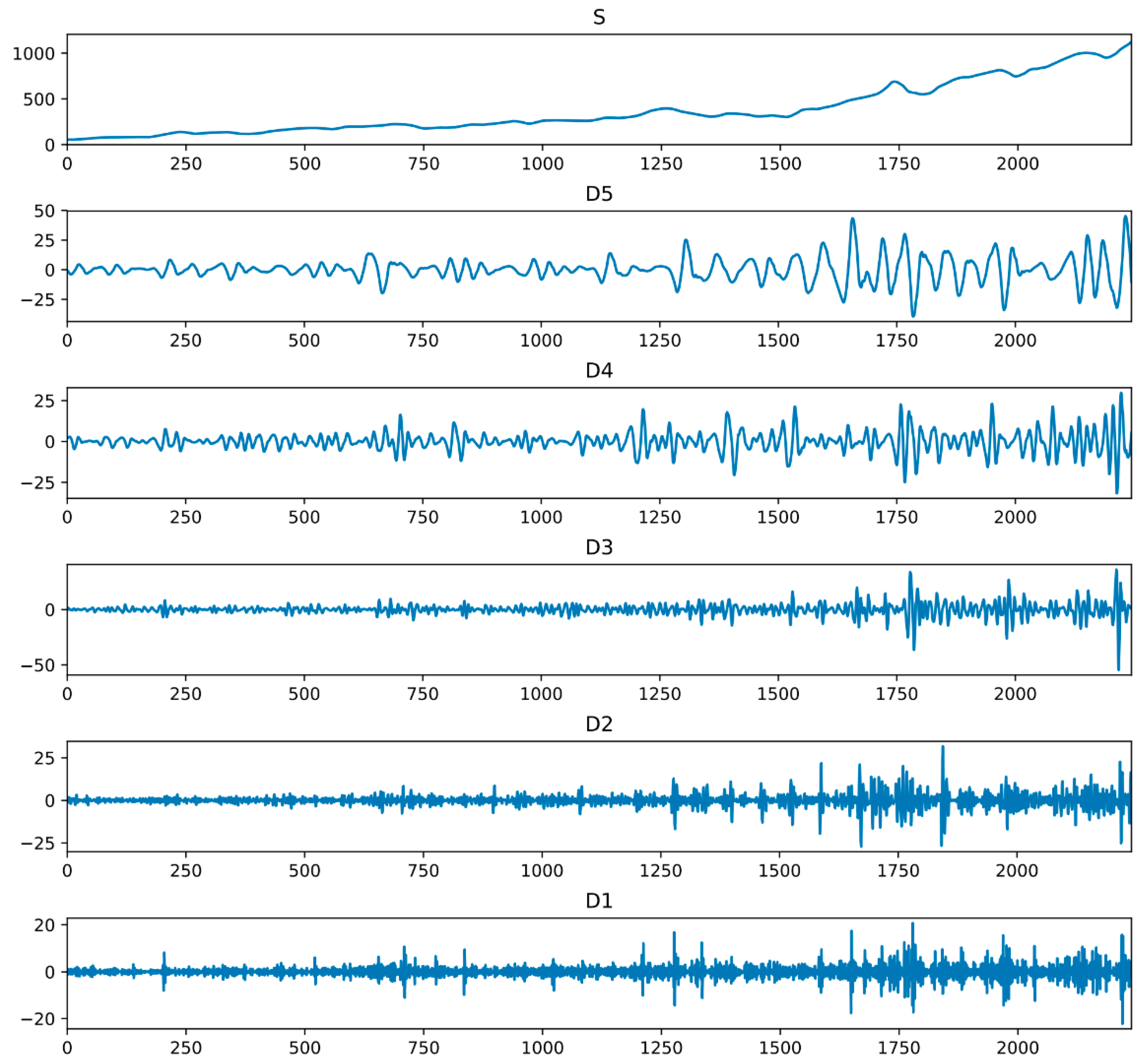
We selected the db4 wavelet as the parent wavelet for the transform. Then, we made the time series data of the decision attribution set into five layers of wavelet decomposition. The first layer to the fifth layer of the wavelet reconstructed signal is shown in Figure 5 As we can observe in this figure, S represents the trend level, and D1–D5 represent the different wavelet decomposition series at different time scales. Here, we obtain five time scales. We can observe that as the scale increases, the image becomes more and more gradual.

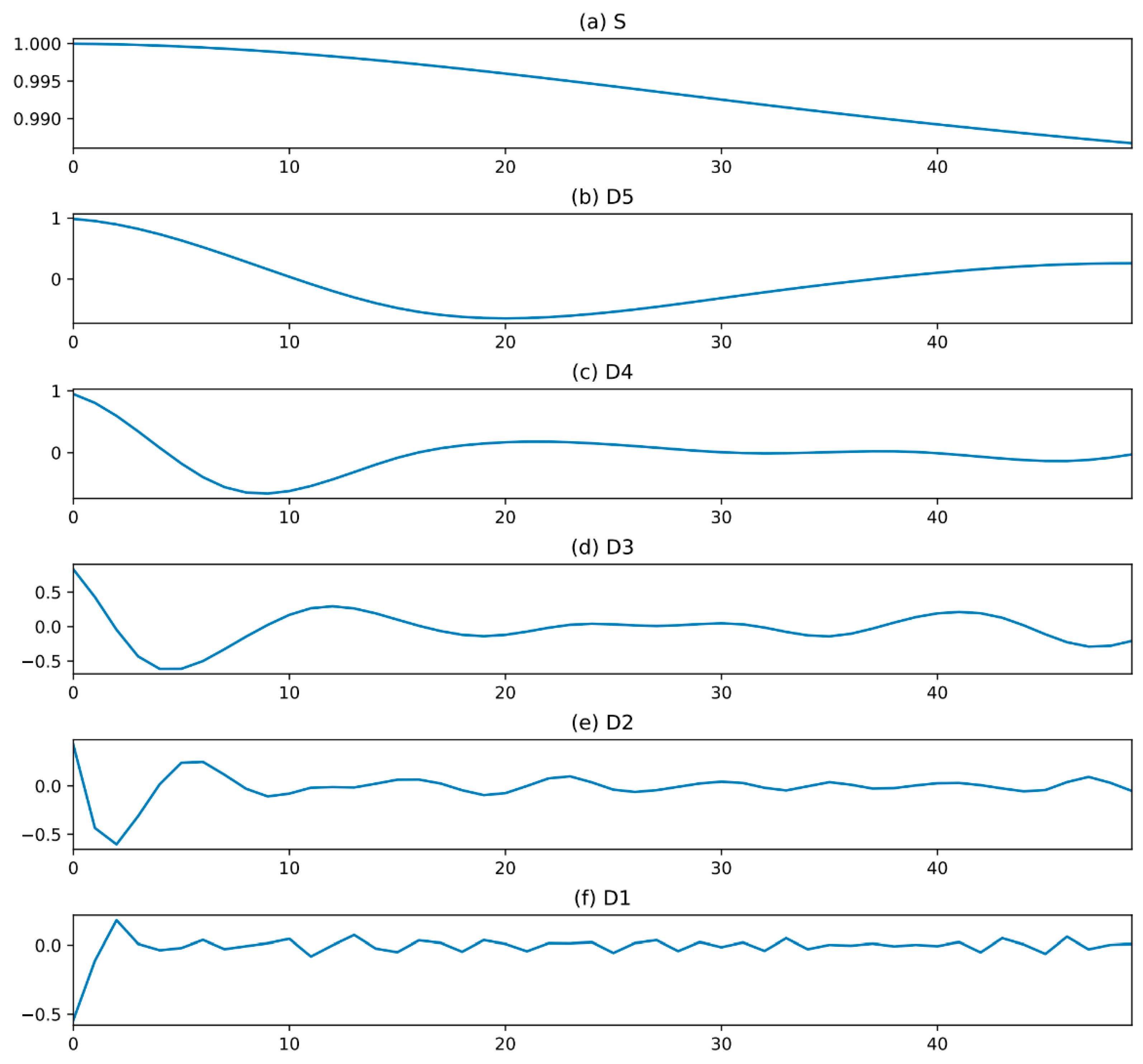
The experimental results for the autocorrelation analysis are shown in Figure 6. It can be observed that the autocorrelation coefficient, which lagged 50 steps from the low-frequency signal of S, is still higher than 0.8. The memory detail of the wavelet coefficients D2 and D1 are less than ten days, so these two wavelet coefficients should be reduced. Leaving the scale coefficients S, and the wavelet coefficients D5, D4, and D3, with memory lengths of more than ten days, are subjected to cross-correlation analysis.

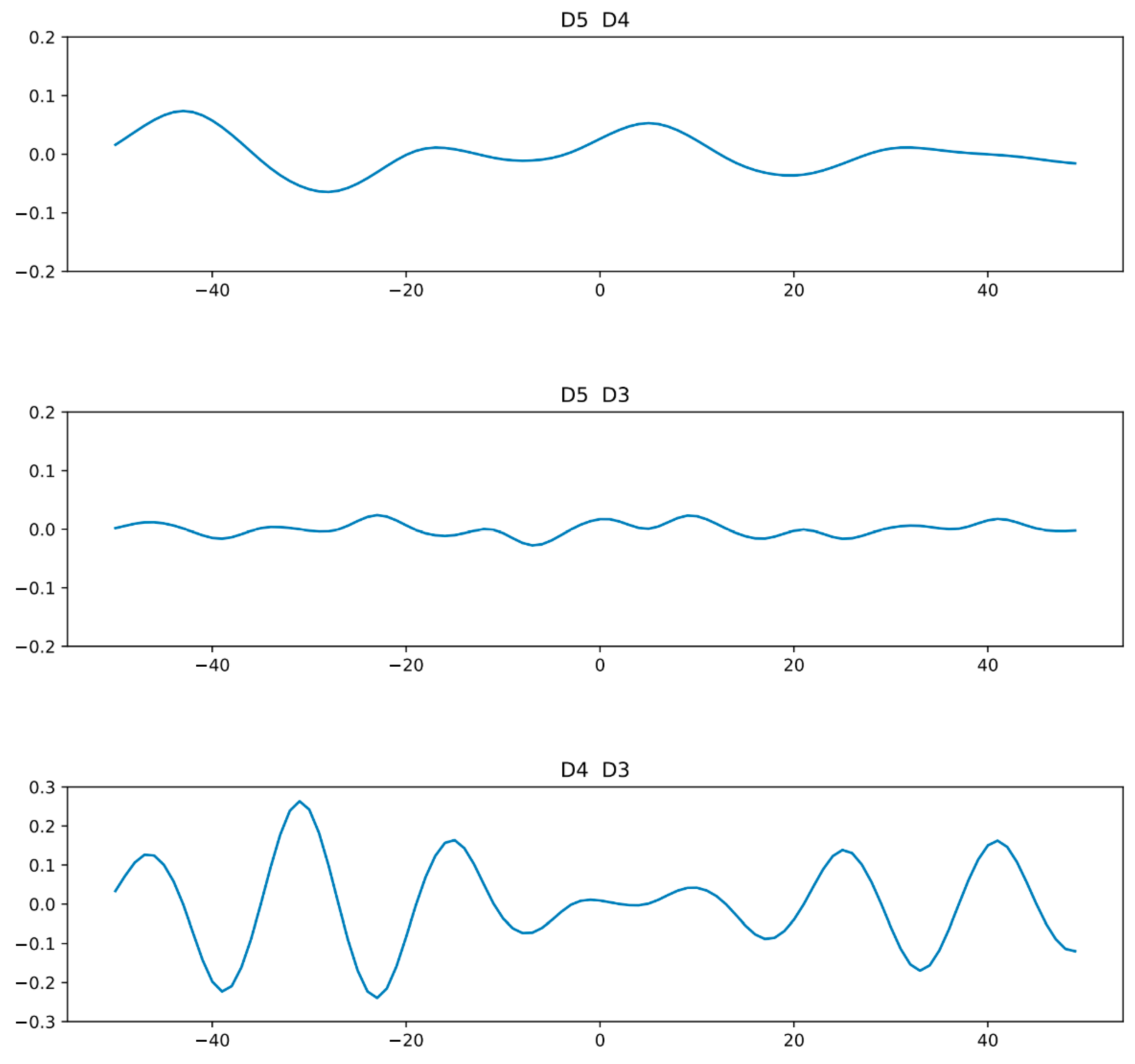
Since S represents the trend information that has a significant effect on the prediction, and S also has the strongest memory for an extended period, the scale coefficient S is directly analyzed for the trend. So, now we conducted cross-correlation analysis for the wavelet coefficients D5, D4, and D3, with the experimental results shown in Figure 7.

It can be observed from Figure 7 that the correlation between the adjacent two wavelet coefficients D5 and D4, and D4 and D3 is active, while the correlation between the separated wavelet coefficients D5 and D3 is weak. Thus, we removed D4, which was associated with the other two wavelets coefficients, and kept the wavelet coefficients D5 and D3, and the scale coefficient S.

4.3. Results and Analysis

4.3.1. Comparisons Results with Other Baseline Algorithms

Table 3. Comparisons results with other algorithms in F1 score.

Stock Industries	Baseline			Our Model
	Bayesian	RF	ANN	DNN
Financials	0.60	0.61	0.63	0.71
Energy	0.56	0.61	0.69	0.65
Technology	0.59	0.57	0.65	0.69
Motor Vehicles and Parts	0.66	0.58	0.71	0.68
Wholesalers	0.65	0.58	0.72	0.70
Healthcare	0.60	0.60	0.72	0.71
Food and Drug Stores	0.53	0.52	0.63	0.64
Transportation	0.64	0.63	0.76	0.72
Telecommunications	0.60	0.58	0.70	0.69
Retailing	0.62	0.58	0.66	0.68
Food, Beverages and Tobacco	0.58	0.56	0.67	0.67
Materials	0.66	0.65	0.71	0.72
Industrials	0.65	0.62	0.76	0.74
Aerospace and Defense	0.65	0.64	0.70	0.71
Engineering and Construction
Chemicals
Business Services
Household Products	0.68	0.63	0.72	0.71
Media	0.59	0.57	0.66	0.68
Apparel	0.64	0.57	0.68	0.68
Hotels, Restaurants and Leisure
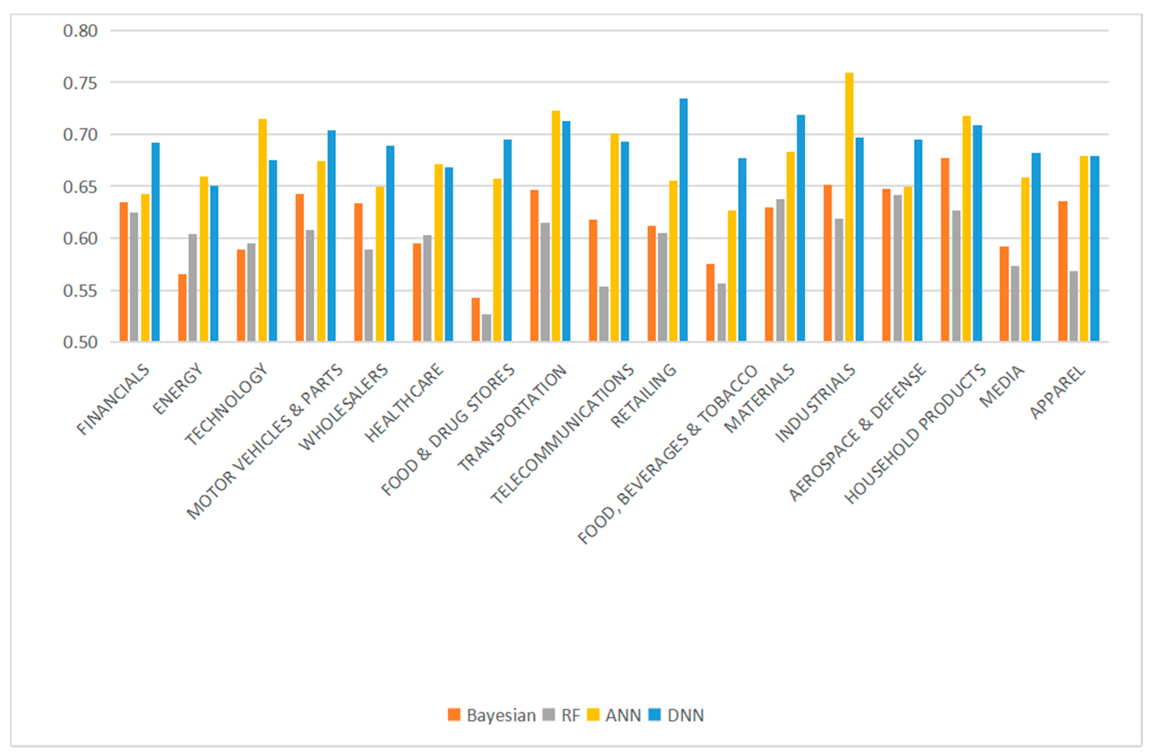
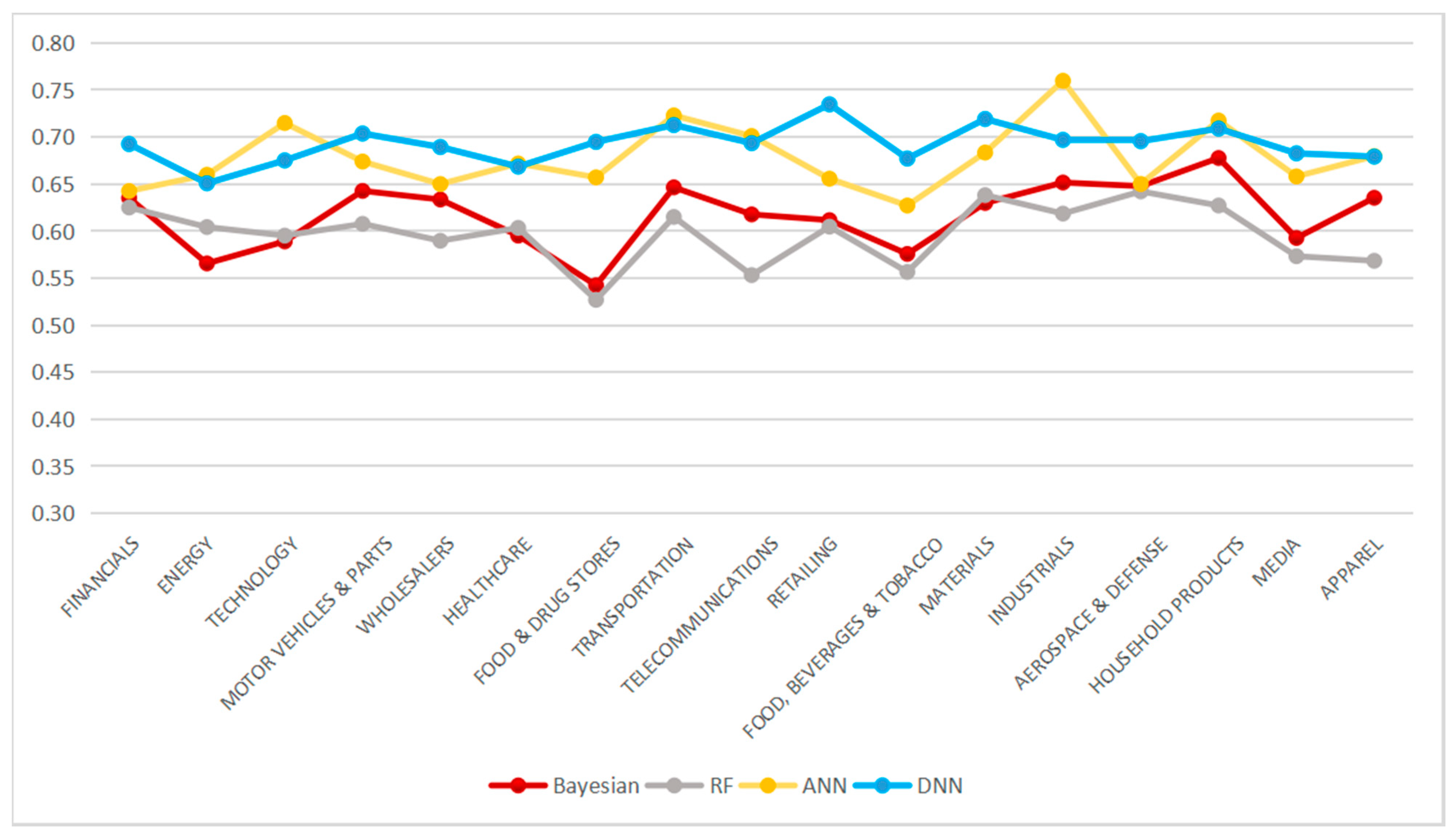
AVG	0.62	0.59	0.69	0.69

shows the results of F1 score. We first calculated the result for each of the 168 stocks, and then we calculated the average for each of the 21 industries. Table 3 also shows the result among different industries, for easy comparison. Using deep neural networks achieved the best result, with a 75% average accuracy for 168 stocks. After using wavelet decomposition of the original time series data, we used other machine learning methods in addition to deep neural networks. The literature shows some machine learning methods, such as decision tree, SVM, Bayesian, ANN, and random forest, which are useful for stock behavior forecasting. We chose the fast and representative new methods among single classifiers and ensemble classifiers. Their results are lower than deep learning, but are better than the 56% hit rate. The nature of our data set strongly influences the performance of a machine learning method.

Compared to most of the other related researchers, our research has some advantages. Firstly, the number of instances (transaction dates) is bigger. We selected the stock price data from the US stock market from 1 January 2009 to 31 December 2017, the data set of which is big enough to capture a high diversity in price movements. Secondly, the number of stocks in our study is more substantial. We studied the behavior of each of the 168 stocks to learn more instances. Thirdly, we used the training and test data on an extended period containing many circumstances, instead of a short period (less than a year). Due to the reasons above, for some stocks, the accuracies are quite high, such as 83.5% for the Alibaba Group Holding stock, and 83.4% for the Toyota Motor stock.

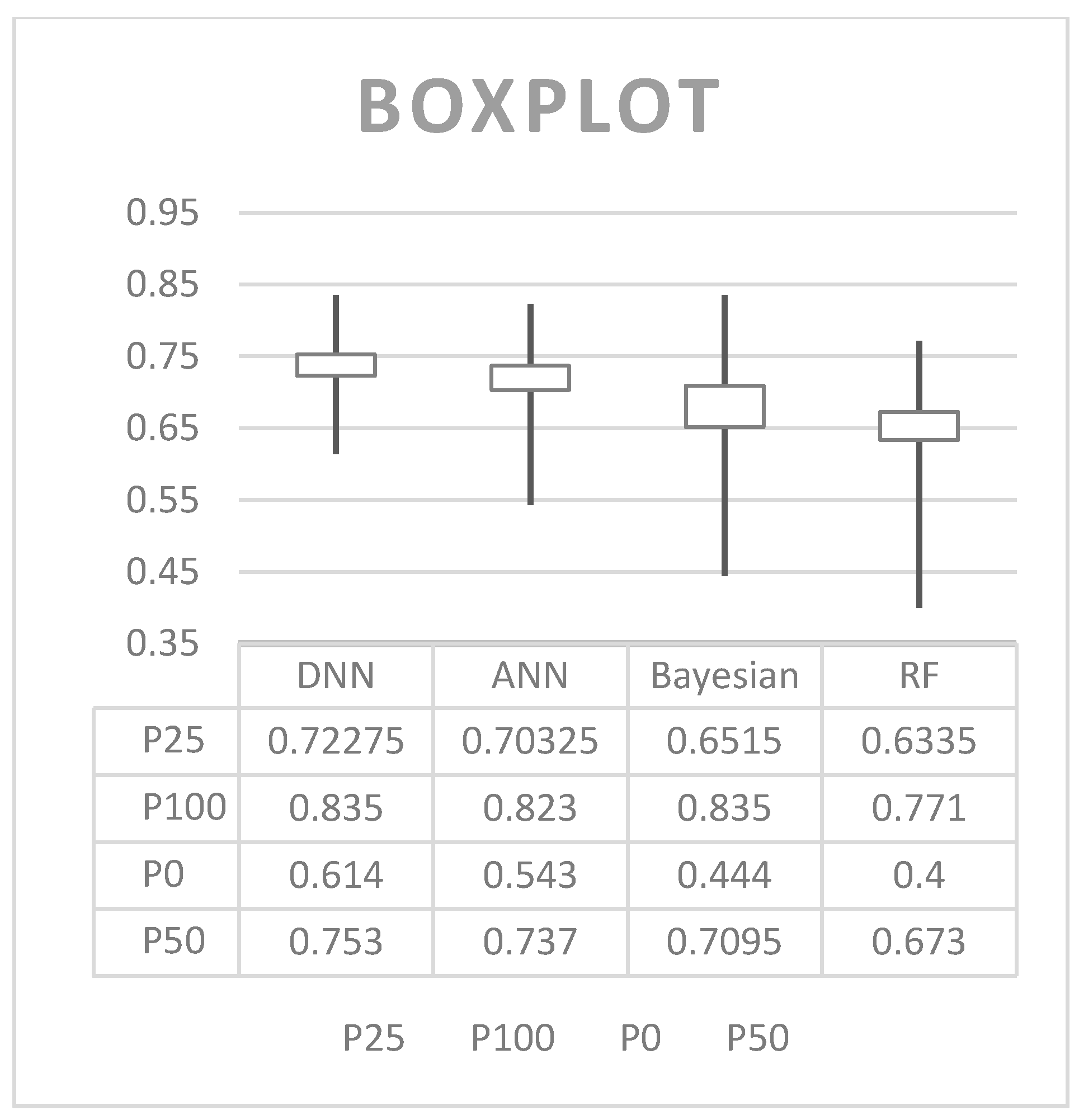
The results of different algorithms reflect differences in machine learning methods. From Figure 8, we can observe that the deep learning method works more stably and reliably than other algorithms. It provides a lower discrete degree and a higher average result than the other three machine learning algorithms. Compared to the regular neural network, DNN shows more-accurate results, but less cost of calculation. However, Bayesian may have an excellent single prediction result, but the overall accuracy is skewed, while RF’s prediction for either stock is not as good as the other three methods.

The main tasks of exploiting ANNs are designing the structure and training the networks. Deep learning allows computational models that are composed of multiple processing layers to learn representations of data with multiple levels of abstraction [44]. The number of hidden layers and neurons in each layer play a vital role in the capacity of a DNN, and no generally accepted theory can determine them [45]. Due to the data types and sample sizes currently obtained, in the case of this paper, the F1 value of the ANN method is close to that of DNN.

4.3.2. Results between Different Industries

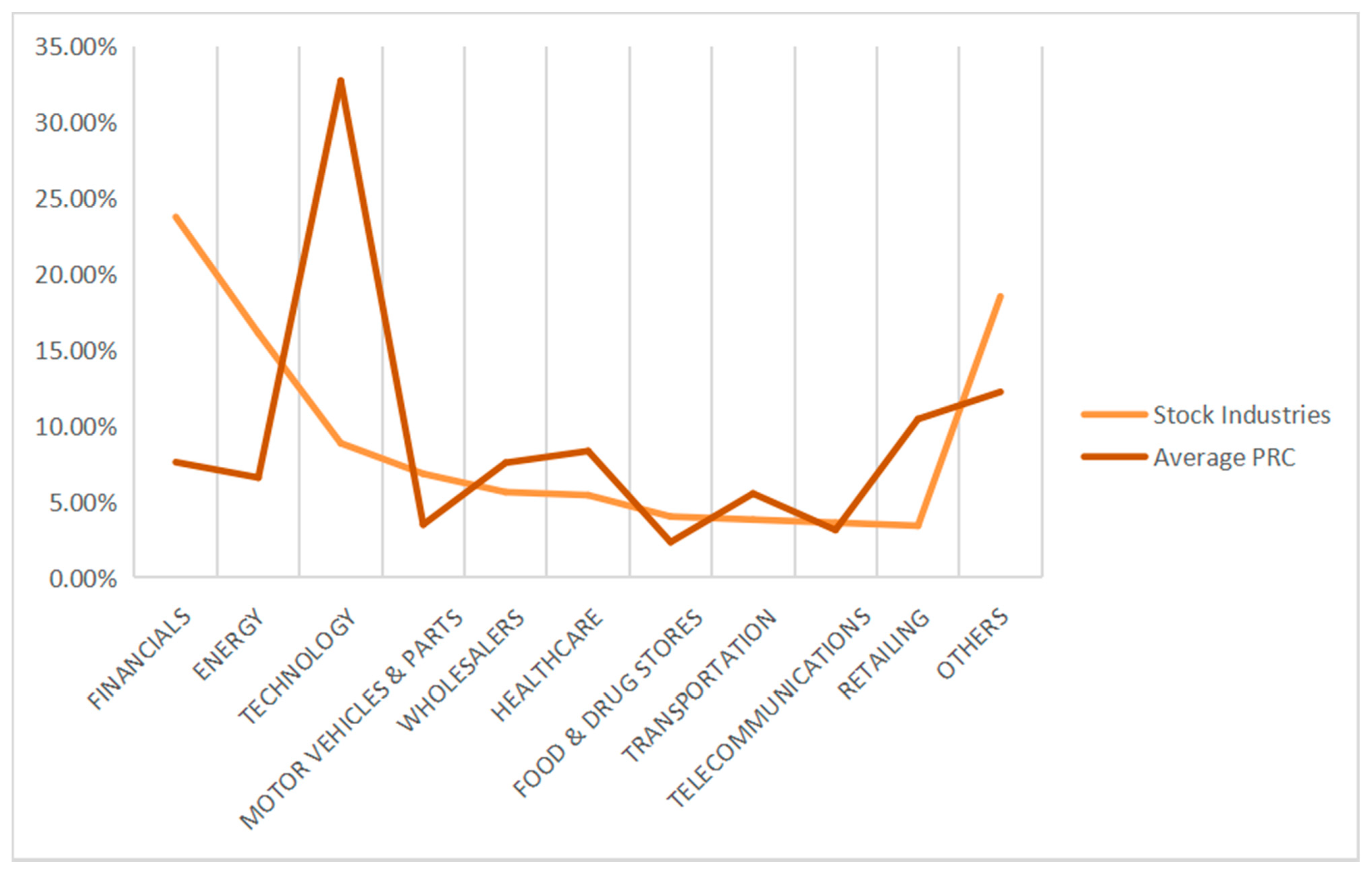
Figure 9 and Figure 10 show the evaluation of the predictive accuracy of different algorithms for different industries. Figure 11 and Figure 12 show the evaluation of the F1 score of different algorithms for different industries. Additionally, Figure 13 shows the overview of PRC and stock industries from 2009 to 2017. Our empirical research characterized the sample with the multi-scale features of the stock market price. In the data preprocessing, some company stocks were unable to be trained because of the short length of the training set. Since this paper does not consider the subsequent processing of such data, we removed these error data from the training and test set. Therefore, as shown in Table 3 and Figure 9 and Figure 10, there are 17 out of 21 industries that have the testing results. There are two more results that can be observed from Table 3 and Figure 9 and Figure 10. Firstly, using our model, the household products industry gets the highest accuracy result, and the apparel industry gets the lowest. One explanation is that these two industries do not have a sufficient number of stocks in this sample, so one single stock will have a significant impact on the industry average. Secondly, in most industries, the DNN prediction results are higher than 75%. Among these, the mean result of DNN for the financial industry, energy industry, and technology industry, which have a large sample of stocks, is roughly 75%. Therefore, the empirical results show that the practical result of our algorithm is higher than 75%. The empirical results also confirm the effectiveness of the method we chose and the model we designed.

5. Conclusions and Future Work

5.1. Conclusions

Stock movement prediction is critical in the financial world. However, it is still an extremely challenging task when facing the non-linear, non-stationary financial time series, which has large-scale features of stock prices. The results of this study support that deep learning is a suitable tool for stock price prediction. In this regard, our study fills the academic research gap of using deep learning in stock movement prediction. Besides deep learning, we found that Bayesian may have an excellent single prediction result, but the overall accuracy is skewed, while random forest’s prediction for either stock is not as good as the other classifiers. Wavelet analysis has good time-frequency local characteristics and good zooming capability for non-stationary random signals. However, the application of the wavelet theory is generally limited to a small scale. The neural networks method is a powerful tool to deal with large-scale problems. Wavelet transform is often compared with Fourier transform, in which signals are represented as a sum of sinusoids. In fact, the Fourier transform can be viewed as a special case of the continuous wavelet transform, with the choice of the mother wavelet. The main difference, in general, is that wavelets are localized in both time and frequency, whereas the standard Fourier transform is only localized in frequency. The short-time Fourier transform (STFT) is similar to wavelet transform, in that it is also time and frequency localized, but there are issues with the frequency/time resolution trade-off. Therefore, the combination of neural networks and wavelet analysis becomes more applicable for stock behavior prediction. By adoption of this combination approach, we perform an empirical study to show the forecast results. This study used deep learning to train the large stock data and find out the accuracy results more significantly than other algorithms. Our test result shows a 75% hit rate, on average, for all industries of the US stocks listed on FT Global 500. In this study, it is demonstrated that multiresolution analysis with the recurrent neural networks method, on the US stock data set, can improve the accuracy of stock movement prediction compared to the conventional neural networks. With the results of our study, we fill the academic research gap by proving that deep learning can be used in stock movement prediction. This study’s primary contribution is to demonstrate a model for reconstructing the stock time series and to perform recurrent neural networks using the deep learning method. Our research contributes to decision makers’ ability to better observe the medium-term behavior of stock markets. Additionally, our method could be used to forecast the behavior of other financial products with multi-scale characteristics, such as the foreign exchange or futures markets, etc.

5.2. Future Work

There is much more work needed to conduct before providing the best suggestion for an investment decision. In fact, the environmental factors and external events have a major impact on stock price, and stock forecasting is a systematic and complex problem. The forecast method in this paper belongs to the technical forecast [12]. Our future work contains the following aspects. On the one hand, on the decision-making aspect, we will continually work on how the stock behavior will affect the investment decisions, by working on trading strategies with the prediction of stock movement. On the other hand, on the deep learning algorithms aspect, we will go more in-depth with the vector details, to find the effectiveness and the cross effect of each other. Besides, due to our research, for some stocks, the accuracies are quite high, such as 83.5% for the Alibaba Group Holding stock, and 83.4% for the Toyota Motor stock. We will go deeper into such stocks or companies to find the reason for that. In the end, in the finance and accounting aspect, there is more exciting work to do when considering the trading volume and the accounting indicators.

References

1. Ballings, M.; Poel, D.V.D.; Hespeels, N.; Gryp, R. Evaluating multiple classifiers for stock price direction prediction. Expert Syst. Appl. 2015, 42, 7046–7056. [Google Scholar] [CrossRef]
2. Chong, E.; Han, C.; Park, F.C. Deep learning networks for stock market analysis and prediction: Methodology, data representations, and case studies. Expert Syst. Appl. 2017, 83, 187–205. [Google Scholar] [CrossRef] [Green Version]
3. Guresen, E.; Kayakutlu, G.; Daim, T.U. Using artificial neural network models in stock market index prediction. Expert Syst. Appl. 2011, 38, 10389–10397. [Google Scholar] [CrossRef]
4. Hsu, C.-M. A hybrid procedure for stock price prediction by integrating self-organizing map and genetic programming. Expert Syst. Appl. 2011, 38, 14026–14036. [Google Scholar] [CrossRef]
5. Thanh, H.T.P.; Meesad, P. Stock Market Trend Prediction Based on Text Mining of Corporate Web and Time Series Data. J. Adv. Comput. Intell. Intell. Inform. 2014, 18, 22–31. [Google Scholar] [CrossRef]
6. Dan, J.; Guo, W.; Shi, W.; Fang, B.; Zhang, T. PSO Based Deterministic ESN Models for Stock Price Forecasting. J. Adv. Comput. Intell. Intell. Inform. 2015, 19, 312–318. [Google Scholar] [CrossRef]
7. Lei, L. Wavelet Neural Network Prediction Method of Stock Price Trend Based on Rough Set Attribute Reduction. Appl. Soft Comput. 2018, 62, 923–932. [Google Scholar] [CrossRef]
8. Chen, Y.; Hao, Y. A feature weighted support vector machine and K-nearest neighbor algorithm for stock market indices prediction. Expert Syst. Appl. 2017, 80, 340–355. [Google Scholar] [CrossRef]
9. Addison, P.S. The Illustrated Wavelet Transform Handbook: Introductory Theory and Applications in Science, Engineering, Medicine and Finance; CRC Press: Boca Raton, FL, USA, 2017. [Google Scholar]
10. Bengio, Y. Learning Deep Architectures for AI. Found. Trends® Mach. Learn. 2009, 2, 1–127. [Google Scholar] [CrossRef]
11. Malkiel, B.G.; Fama, E.F. Efficient Capital Markets: A Review of Theory and Empirical Work. J. Financ. 1970, 25, 383–417. [Google Scholar] [CrossRef]
12. Singh, R.; Srivastava, S. Stock prediction using deep learning. Multimed. Tools Appl. 2017, 76, 18569–18584. [Google Scholar] [CrossRef]
13. Tsinaslanidis, P.; Kugiumtzis, D. A prediction scheme using perceptually important points and dynamic time warping. Expert Syst. Appl. 2014, 41, 6848–6860. [Google Scholar] [CrossRef]
14. Schumaker, R.P.; Chen, H. A quantitative stock prediction system based on financial news. Inf. Process. Manag. 2009, 45, 571–583. [Google Scholar] [CrossRef]
15. Tsibouris, G.; Zeidenberg, M. Testing the efficient markets hypothesis with gradient descent algorithms. In Neural Networks in the Capital Markets; Wiley: Chichester, UK, 1995; pp. 127–136. [Google Scholar]
16. Thomsett, M.C. Mastering Fundamental Analysis; Dearborn Financial Publishing: Chicago, IL, USA, 1998. [Google Scholar]
17. Thomsett, M.C. Mastering Technical Analysis; Dearborn Trade Publishing: Chicago, IL, USA, 1999. [Google Scholar]
18. Hellström, T.; Holmström, K. Predictable Patterns in Stock Returns. Sweden. 1998. Available online: http://citeseerx.ist.psu.edu/viewdoc/summary?doi=10.1.1.12.8541 (accessed on 7 September 2021).
19. Teixeira, L.A.; de Oliveira, A.L.I. A method for automatic stock trading combining technical analysis and 1998 nearest neighbor classification. Expert Syst. Appl. 2010, 37, 6885–6890. [Google Scholar] [CrossRef]
20. Hagenau, M.; Hauser, M.; Liebmann, M.; Neumann, D.; Neumann, D. Reading All the News at the Same Time: Predicting Mid-term Stock Price Developments Based on News Momentum. In Proceedings of the 2013 46th Hawaii International Conference on System Sciences, Maui, HI, USA, 7–10 January 2013; pp. 1279–1288. [Google Scholar]
21. Daubechies, I. Ten Lectures on Wavelets; SIAM: Philadelphia, PA, USA, 1992. [Google Scholar]
22. Chen, A.-S.; Leung, M.T.; Daouk, H. Application of neural networks to an emerging financial market: Forecasting and trading the Taiwan Stock Index. Comput. Oper. Res. 2003, 30, 901–923. [Google Scholar] [CrossRef]
23. Hadavandi, E.; Shavandi, H.; Ghanbari, A. Integration of genetic fuzzy systems and artificial neural networks for stock price forecasting. Knowl. Based Syst. 2010, 23, 800–808. [Google Scholar] [CrossRef]
24. Kim, K.-J.; Han, I. Genetic algorithms approach to feature discretization in artificial neural networks for the prediction of stock price index. Expert Syst. Appl. 2000, 19, 125–132. [Google Scholar] [CrossRef]
25. Rather, A.M.; Agarwal, A.; Sastry, V. Recurrent neural network and a hybrid model for prediction of stock returns. Expert Syst. Appl. 2015, 42, 3234–3241. [Google Scholar] [CrossRef]
26. Saad, E.; Prokhorov, D.; Wunsch, D. Comparative study of stock trend prediction using time delay, recurrent and probabilistic neural networks. IEEE Trans. Neural Netw. 1998, 9, 1456–1470. [Google Scholar] [CrossRef]
27. Ticknor, J.L. A Bayesian regularized artificial neural network for stock market forecasting. Expert Syst. Appl. 2013, 40, 5501–5506. [Google Scholar] [CrossRef]
28. Nagaya, S.; Chenli, Z.; Hasegawa, O. A Proposal of Stock Price Predictor Using Associated Memory. J. Adv. Comput. Intell. Intell. Inform. 2011, 15, 145–155. [Google Scholar] [CrossRef]
29. White, H. Economic prediction using neural networks: The case of IBM daily stock returns. In Proceedings of the IEEE International Conference on Neural Networks, San Diego, CA, USA, 24–27 July 1988. [Google Scholar]
30. Wuthrich, B.; Cho, V.; Leung, S.; Permunetilleke, D.; Sankaran, K.; Zhang, J. Daily stock market forecast from textual web data. In Proceedings of the SMC’98 Conference Proceedings—1998 IEEE International Conference on Systems, Man, and Cybernetics (Cat. No.98CH36218), San Diego, CA, USA, 14 October 1998; Volume 1–5, pp. 2720–2725. [Google Scholar]
31. Groth, S.S.; Muntermann, J. An intraday market risk management approach based on textual analysis. Decis. Support Syst. 2011, 50, 680–691. [Google Scholar] [CrossRef]
32. Enke, D.; Mehdiyev, N. Stock Market Prediction Using a Combination of Stepwise Regression Analysis, Differential Evolution-based Fuzzy Clustering, and a Fuzzy Inference Neural Network. Intell. Autom. Soft Comput. 2013, 19, 636–648. [Google Scholar] [CrossRef]
33. Chiang, W.-C.; Enke, D.; Wu, T.; Wang, R. An adaptive stock index trading decision support system. Expert Syst. Appl. 2016, 59, 195–207. [Google Scholar] [CrossRef]
34. Arévalo, A.; Niño, J.; Hernández, G.; Sandoval, J. High-Frequency Trading Strategy Based on Deep Neural Networks. In Intelligent Computing Methodologies; Huang, D.S., Han, K., Hussain, A., Eds.; Lecture Notes in Computer Science; Springer: Cham, Switzerland, 2016; Volume 9773. [Google Scholar] [CrossRef] [Green Version]
35. Zhong, X.; Enke, D. Forecasting daily stock market return using dimensionality reduction. Expert Syst. Appl. 2017, 67, 126–139. [Google Scholar] [CrossRef]
36. Ejbali, R.; Zaied, M. A dyadic multi-resolution deep convolutional neural wavelet network for image classification. Multimed. Tools Appl. 2018, 77, 6149–6163. [Google Scholar] [CrossRef]
37. Siegelmann, H.T.; Sontag, E. Turing computability with neural nets. Appl. Math. Lett. 1991, 4, 77–80. [Google Scholar] [CrossRef] [Green Version]
38. Zhang, Q.; Benveniste, A. Wavelet networks. IEEE Trans. Neural Netw. 1992, 3, 889–898. [Google Scholar] [CrossRef]
39. Zhang, J.; Walter, G.; Miao, Y.; Lee, W.N.W. Wavelet neural networks for function learning. IEEE Trans. Signal Process 1995, 43, 1485–1497. [Google Scholar] [CrossRef]
40. Bakshi, B.; Stephanopoulos, G. Wave-net: A multiresolution, hierarchical neural network with localized learning. Aiche J. 1993, 39, 57–81. [Google Scholar] [CrossRef]
41. Yamanaka, S.; Morikawa, K.; Yamamura, O.; Morita, H.; Huh, J.Y. The Wavelet Transform of Pulse Wave and Electrocardiogram Improves Accuracy of Blood Pressure Estimation in Cuffless Blood Pressure Measurement. Circulation 2016, 134 (Suppl. 1), A14155. [Google Scholar]
42. Xu, M. Study on the Wavelet and Frequency Domain Methods of Financial Volatility Analysis. Ph.D. Thesis, Tianjin University, Tianjin, China, 2004. [Google Scholar]
43. Al Shalabi, L.; Shaaban, Z.; Kasasbeh, B. Data Mining: A Preprocessing Engine. J. Comput. Sci. 2006, 2, 735–739. [Google Scholar] [CrossRef] [Green Version]
44. LeCun, Y.; Bengio, Y.; Hinton, G. Deep learning. Nature 2015, 521, 436–444. [Google Scholar] [CrossRef] [PubMed]
45. Deng, J.; Sun, J.; Peng, W.; Hu, Y.; Zhang, D. Application of neural networks for predicting hot-rolled strip crown. Appl. Soft Comput. 2019, 78, 119–131. [Google Scholar] [CrossRef]
Figure 1. Difference between deep learning and the traditional machine learning process.
Information 12 00388 g001
Figure 2. Forward propagation of deep neural networks with four layers.
Information 12 00388 g002
Figure 3. The flowchart of the proposed algorithm.
Information 12 00388 g003
Figure 4. A model of multiresolution analysis used for stock price prediction.
Information 12 00388 g004
Figure 5. Multi-scale analysis for day closing price (PRC).
Information 12 00388 g005
Figure 6. Autocorrelation analysis results for multi-scale coefficients.
Information 12 00388 g006
Figure 7. Cross-correlation analysis results for multi-scale coefficients.
Information 12 00388 g007
Figure 8. Boxplot between different algorithms.
Information 12 00388 g008
Figure 9. The evaluation of predictive accuracies in industries.
Information 12 00388 g009
Figure 10. The evaluation of predictive accuracies in industries.
Information 12 00388 g010
Figure 11. The evaluation of F1 score in industries.
Information 12 00388 g011
Figure 12. The evaluation of F1 score in industries.
Information 12 00388 g012
Figure 13. Overview of average PRC and stock industries (2009 to 2017).
Information 12 00388 g013