The Two-Layer Hierarchical Distribution Model of Zeros of Riemann’s Zeta Function along the Critical Line

Abstract

This article numerically analyzes the distribution of the zeros of Riemann’s zeta function along the critical line (CL). The zeros are distributed according to a hierarchical two-layered model, one deterministic, the other stochastic. Following a complex plane anamorphosis involving the Lambert function, the distribution of zeros along the transformed CL follows the realization of a stochastic process of regularly spaced independent Gaussian random variables, each linked to a zero. The value of the standard deviation allows the possible overlapping of adjacent realizations of the random variables, over a narrow confidence interval. The hierarchical model splits the $\zeta$ function into sequential equivalence classes, with the range of probability densities of realizations coinciding with the spectrum of behavioral styles of the classes. The model aims to express, on the CL, the coordinates of the alternating cancellations of the real and imaginary parts of the $\zeta$ function, to dissect the formula for the number of zeros below a threshold, to estimate the statistical laws of two consecutive zeros, of function maxima and moments. This also helps explain the absence of multiple roots.

1. Introduction

This article presents a distribution model of the non-trivial zeros of the zeta function on the critical line (CL). The Riemann Hypothesis (RH) [1] places them exclusively on this line, but this article focuses on the CL zeros, regardless of the RH.

We first explored the global behavior of the $\zeta$ function on the CL, and the role of the Lambert function [2] on the folds of the $\zeta$ function in the critical strip (CS). A close relationship exists, on the CL, between Riemann’s $\zeta$ function and Lambert’s $W$ function, after an anamorphosis of the ordinate of the complex plane.

This article also shows that, on the CL, there is a relationship between both the real and imaginary components of the $\zeta$ function. This ratio, only valid on the CL, takes into account an angle tied to the fractional part of the anamorphosed ordinate, which makes it possible to anchor the common zeros of these two components in an equivalence relation, where the classes are intervals of unit length. Thus, both $\zeta$ surfaces, alternatingly zero, with period one on the anamorphosed ordinate of the complex plane, locally generate an additional common zero which is the $n$th non-trivial zero.

The article then investigates, on the anamorphosed axis, the local “random” character of the $n$th non-trivial zero, in the form of the realization of a Gaussian random variable (RV) with a mean $n$ and standard deviation ${\tilde{\sigma }}_n$ increasing very slowly with $W\left(\ln n\right)$, of order $\raisebox{1ex}{$1$}\!\left/ \!\raisebox{-1ex}{$3$}\right.$ for $n < {10}^7$, all these $n$ RVs being pairwise independent. The magnitude of the standard deviation leads to the possible permutation of some realizations of adjacent RVs, justifying the uncertainty in the formula for the number of zeros below a given threshold, and explaining the corresponding difficulty for algorithms to compute these zeros.

Finally, this article presents a taxonomy of the local behaviors of the $\zeta$ function in the CS, according to the probability density of the RV relevant to the $n$th zero. The model still allows a number of derivations which reaffirm some classical formulas of the Riemann $\zeta$ function. This also helps explain the absence of multiple roots.

By consulting the abundant scientific literature on the zeros of the Riemann $\zeta$ function, including certain pioneering articles [3,4,5,6,7,8], one can distinguish three broad families of publications, with the first two having the underlying ambition to provide proof of the RH.

The first family consists in circumscribing the perimeter of the region where the zeros are located. As early as 1896, Hadamard [3] and La Vallée Poussin [4] restricted the “fertile region” of zeros to the CS $\left(0<x<1\right)$. Then, during the twentieth century, the region was reduced in two ways. On the one hand, by further limiting the perimeter, and on the other hand by increasing the percentage of potential zeros on or around the CL [9,10], in an increasingly restricted perimeter.

The second family consists in analyzing only CL zeros [11,12], by estimating the number of zeros less than a $y$ value of the ordinate of $s$ [13], by calculating the number of zero crossings on the CL, by studying the adjacent zeros, or by estimating other characteristics of the $\zeta$ function, always with the aim of apprehending the RH, according to various points of view.

The third family, more concretely, consists in effectively calculating the CL zeros with a numerical algorithm [14,15]. Currently, the exercise, which thrived between 1985 and 2005, has seen a loss of momentum, as the number of known zeros is substantial. Extending these calculations has become superfluous with silicon computers, although searches for zeros beyond about $n > {10}^{100}$ over an interval of the order of $\Delta n={10}^{10}$, would provide interesting additional knowledge on the $\zeta$ function.

The aim of this article belongs to the second family, by taking advantage of numerical results of the third family. Indeed, the goal here is not to investigate questions about the RH, nor to determine an algorithm to effectively calculate zeros. The goal is mainly to define, on the CL, a distribution model with two layers, one deterministic and the other stochastic, to specify the local characteristics of the $\zeta$ function around the zeros and to discuss the evolution of local behavior of rare events with increasing $n$.

Despite its age, Edward Charles Titchmarsh’s book [16] is the most comprehensive book on $\zeta$ function theory. It covers almost everything anyone would want to know about the $\zeta$ function. Aleksandar Ivić’s book (Александар Ивић) [17] offers an easier approach for anyone who wants to understand all of the questions about the $\zeta$ function, including the theory but also its applications.

After this introduction, the notations, methodology, data, computer science and mathematical tools are presented in Section 2. Section 3 presents the results. A discussion of the assumptions and results is expressed in Section 4, before the conclusion. The whole article is based on numerical calculations performed by computer programs in the Python language, designed and implemented by the author. Some calculations are supported by power series, which were validated by computer.

2. Materials and Methods

2.1. Mathematical Notations

Where possible, classical mathematical notations have been selected (Table 1): to lighten the writing, some original notations are defined.

Table 1. Notations.

Definition	Notation
Absolute value	$\forall a∊\mathbb{R}: \left|a\right|=a if a>0;-a if a<0$
Complex number	$\forall z\in \mathbb{C}:z=x+iy=r{e}^{i\theta }=\left|z\right|e^{i arg\left(z\right)};$ $\left|z\right|=\left|x+iy\right|=\sqrt{x^2+y^2} ;x,y, r, \theta \in \mathbb{R}$ $\theta =arctan\left(y/x\right) modulo 2\pi if x>0;$ $\theta =arctan\left(y/x\right) modulo \pi +\pi if x<0;$ $x=0: \theta =\pi /2 if y>0; \theta =-\pi /2 if y<0$
Integer and fractional parts	In $\mathbb{R}$, the integer part and the fractional part of a real number $a$: $\forall a∊\mathbb{R}:a=\left[a\right]+\left\{a\right\}; \left[a\right]∊\mathbb{N}, 0\le \left\{a\right\}<1$
Complex number in the CS	In $\mathbb{C}$, $s=x+i y=\mathfrak{R}\left(s\right)+i \mathfrak{I}\left(s\right);s\in \mathbb{C};x, y∊\mathbb{R};$ its conjugate $\overline{s}=x-i y$
Complex number $1-s$ associated with $s$	In $\mathbb{C}$, $\widehat{s}=1-s=1-x-i y;x, y∊\mathbb{R};$ its conjugate $\check{s}=\overline{1-s}=\overline{\widehat{s}}=1-x+i y$. $\widehat{s}$ symmetric of $s$ with respect to ($\raisebox{1ex}{$1$}\!\left/ \!\raisebox{-1ex}{$2$}\right.,0$).
Critical strip (CS)	In the CS $\mathcal{S}$: $s=\mathfrak{R}\left(s\right)+i \mathfrak{I}\left(s\right)= x+i y; 0\le x\le 1, y>0; s\ne 1$.
Critical line (CL)	On the CL $\mathcal{L}:=x=\raisebox{1ex}{$1$}\!\left/ \!\raisebox{-1ex}{$2$}\right.$: $𝓈=\raisebox{1ex}{$1$}\!\left/ \!\raisebox{-1ex}{$2$}\right.+i𝓎; 𝓎>0$.
CS, except the CL	$\mathcal{S}\backslash \mathcal{L}:=0\le x\le 1;x\ne \raisebox{1ex}{$1$}\!\left/ \!\raisebox{-1ex}{$2$}\right.; s\ne 1$
Zeta function: $\zeta$	$\zeta \left(s\right)={{\displaystyle \sum }}_1^{\infty }{n}^{-s}.$ In the CS, the $\zeta$ function is divergent. One considers in this CS, the analytical continuation $\eta \left(s\right)$.
Êta Dirichlet function: $\eta$	$\eta \left(s\right)=\zeta \left(s\right)\left(1-2^{-s+1}\right)$.
Derivative of the $\zeta$ function	${\zeta }^{\prime }\left(s\right)=-{{\displaystyle \sum }}_{n=1}^{\infty }\log \left(n\right)/n^s$
k-order derivatives of the $\zeta$ function	${\zeta }^{\left(k\right)}\left(s\right)={{\displaystyle \sum }}_{n=1}^{\infty }{\left(-\log \left(n\right)\right)}^k/n^s$ In the CS, one uses the analytical continuation of these derivatives
Functional equation of the $\zeta$ function	$\zeta \left(s\right)=\xi \left(s\right)\zeta \left(\widehat{s}\right)=\xi \left(s\right)\zeta \left(1-s\right)$ $\xi \left(s\right)=2^s{\pi }^{s-1}\sin \left(\pi s/2\right)\mathsf{\Gamma }\left(1-s\right)={\pi }^{s-\raisebox{1ex}{$1$}\!\left/ \!\raisebox{-1ex}{$2$}\right.}\frac{\mathsf{\Gamma }\left(\widehat{s}/2\right)}{\mathsf{\Gamma }\left(s/2\right)}$
Functional equation on the CL	$\zeta \left(𝓈\right)=\xi \left(𝓈\right)\zeta \left(\widehat{𝓈}\right)=\xi \left(𝓈\right)\zeta \left(\overline{𝓈}\right)=\xi \left(𝓈\right)\overline{\zeta }\left(𝓈\right);$ $\xi \left(𝓈\right)={\pi }^{i𝓎}\frac{\overline{\mathsf{\Gamma }}\left(𝓈/2\right)}{\mathsf{\Gamma }\left(𝓈/2\right)}$
$t$	$\mathrm{t}=y/\left(2\pi \right)=y/2\pi$
Anamorphosis: $\tilde{t}$	$\tilde{t}=t\ln \left(t/e\right)=y/\left(2\pi \right)\ln \left(y/\left(2\pi e\right)\right)$. The anamorphosis produces a stronger elongation of the $y$ axis as $y$ increases.
Digressive series	We define by the adjective “digressive” a series that exhibits a beginning similar to a known series, but which varies noticeably with the subsequent terms. For example, the cosine series is written: $\cos x=1-\frac{x^2}{2!}+\frac{x^4}{4!}-\frac{x^6}{6!}+\cdots +{\left(-1\right)}^n\frac{x^{2n}}{\left(2n\right)!}+𝒪\left(x^{2n+1}\right)$. We will then note, in order to simplify the writing, a digressive cosine: ${\displaystyle \breve{cos}}\left(x\right)=1-\frac{a_2{x}^2}{2!}+\frac{a_4{x}^4}{4!}-\frac{a_6{x}^6}{6!}+\cdots +{\left(-1\right)}^n\frac{a_{2n}{x}^{2n}}{\left(2n\right)!}+𝒪\left(x^{2n+1}\right)$.
Complex zeros $ℨ$ in the CS $\mathcal{S}$	$z_n=x_n+i y_n; \zeta \left(z_n\right)=0$
Zeros $\mathcal{Z}\subset ℨ$ on the CL $\mathcal{L}\subset \mathcal{S}$	${𝓈}_n=\raisebox{1ex}{$1$}\!\left/ \!\raisebox{-1ex}{$2$}\right.+i {𝓎}_n; \zeta \left({𝓈}_n\right)=0$ The zeros are ordered in pairs, $s$ and $1-s$. Calculations are carried out with $y>0$
Lambert function	The main branch is defined by: $W\left(z\right)=w \iff z=w{e}^w;z\ge -1/e$.
Gamma function	$\mathsf{\Gamma }\left(z\right)={{\displaystyle \int }}_0^{\infty }{t}^{z-1}{e}^{-t}dt$
Euler’s constant	Euler–Mascheroni constant: $\gamma =\underset{n\to \infty }{\lim }\left(-\ln n+{{\displaystyle \sum }}_{k=1}^n\frac{1}{k}\right)\approx 0.5772156649$
Taylor series	$f\left(z\right)={{\displaystyle \sum }}_{n=0}^{\infty }\frac{f^{\left(n\right)}\left(a\right)}{n!}{\left(z-a\right)}^n$
Bernoulli numbers	Coefficients of the power series of $\frac{t}{e^t-1}={{\displaystyle \sum }}_{n=0}^{\infty }{\mathcal{B}}_n\frac{t^n}{n!}$ ${\mathcal{B}}_0=1; {\mathcal{B}}_1=-\raisebox{1ex}{$1$}\!\left/ \!\raisebox{-1ex}{$2$}\right.; if k>0:{\mathcal{B}}_{2k+1}=0 ;{\mathcal{B}}_2=\frac{1}{6};{\mathcal{B}}_4=-\frac{1}{30};{\mathcal{B}}_6=\frac{1}{42};{\mathcal{B}}_8=-\frac{1}{30};{\mathcal{B}}_{10}=\frac{5}{66};{\mathcal{B}}_{12}=-\frac{691}{2730};{\mathcal{B}}_{14}=\frac{7}{6};{\mathcal{B}}_{16}=-\frac{3617}{510};{\mathcal{B}}_{18}=\frac{\mathrm{43,867}}{798}$; ${\mathcal{B}}_{2n}={\left(-1\right)}^{n-1}\left|{\mathcal{B}}_{2n}\right|$; ${\mathcal{B}}_{2n}~{\left(-1\right)}^{n-1}\frac{2\left(2n\right)!}{{\left(2\pi \right)}^{2n}}$

2.2. Numerical and Graphical Observation as a Tool for Reflection

It is fruitful to numerically represent and visualize the catalog of formulas, well known to all, to verify some exact formulas with infinite sums and to validate approximations or inequalities, demonstrated mathematically, to testify to their robustness, speed of convergence and power of truth. Graphical visualization is a powerful tool for analysis and reflection, which amply guides intuition to take paths that are difficult, if not impossible, to take with the traditional manipulation of mathematical formulas. However, the $\zeta$ function calculations become complicated, even impractical, on a computer, when $n$ takes large values ($n>{10}^{100}$). The window of practicable computer calculations ignores large numbers.

2.3. The Gap between Observation and Demonstration

Numerical processing and observation allow for the quashing of a formula, approximation or inequality, with a single representation, when this representation does not conform to the postulate or original intuition. However, the numerical calculation and graphical visualization on the first few million zeros do not demonstrate anything. We know the fallacy of the hasty general conclusions drawn from premature examinations of a phenomenon observed over too small an interval, while the results change or reverse over a wider interval. The well-known example is the Skewes number on the difference $\pi \left(x\right)-Li\left(x\right)$, where the sign swaps for huge values (a current upper bound where this occurs is $1.39822\times {10}^{316}$). For the $\zeta$ function, the profile of the real and imaginary surfaces has more and more tightly packed folds, with increasingly strong amplitudes. The mixing of RVs and the rules for the appearance of zeros undergo very slow evolutions, so that the observations for $n<{10}^{20}$ risk masking new landscapes of the $\zeta$ function for higher values, beyond ${10}^{100}$. A (perhaps daring) extrapolation will nevertheless help to predict the behavior beyond $N={10}^{20}$.

The methodology here consists in first presenting the graphs and statistics on the raw variables. An analysis then allows these variables to undergo geometric transformations, in order to obtain more abstract calculated variables but with classic statistics that can be manipulated, mathematically.

Observation is also a good complementary tool, preceding a demonstration. This is what we will expose by presenting the graphical evolution of the local distribution of consecutive zeros and the evidence for the presence of only single roots in the CS.

2.4. Data and Computer Science Tools Used

This study was performed using the set $\mathcal{D}$, which represents the first 6 million zeros, as well as a few other sets of higher values. On the interval $I:=\{0<y<{10}^{20}\}$, we observe, without exception, that the zeros are located on the CL ($x=\raisebox{1ex}{$1$}\!\left/ \!\raisebox{-1ex}{$2$}\right.$) according to the two-layered model (Lambert function and stochastic Laplace–Gauss process) described below. To obtain the list of zeros on the CL, one can consult several websites on the Internet [14,15], but one can also recalculate some of them. The computer used by the author is a personal computer, and therefore certain calculations sometimes take an exorbitant processing time: the calculation of certain zeros takes days of calculation time to obtain.

All the programs were written in Python, with the graphics library matplotlib and the mathematical library mpmath to allow for calculations with a number of adjustable significant figures (in the order of 15, 30 or 50, depending on the case) for floating point numbers.

2.5. Mathematical Tools Used

2.5.1. Stochastic Processes

$Y_n$ is a random variable (an RV). The RVs $Y_n$ are pairwise independent RVs.

${\tilde{T}}_n$ is a Gaussian RV ${\tilde{T}}_n~\mathcal{N}\left({\tilde{\mu }}_n,{\tilde{\sigma }}_n^2\right)$. The RVs ${\tilde{T}}_n$ are pairwise independent.

The two-layer hierarchical model $ℳ$ is:

An anamorphosis $\phi$ from $\mathbb{C}$ to $\tilde{\mathbb{C}}$:

$$\phi : \mathcal{S}\subset \mathbb{C} \to \tilde{\mathcal{S}}\subset \tilde{\mathbb{C}}$$

$$M:\left(x,y\right)\to \tilde{M}:\left(x, \tilde{t}\right)=\phi \left(M\right) ; \tilde{t}=t \ln \left(t/e\right);t=y/2\pi$$

Two stochastic processes $\left\{Y\right\}$ and $\left\{T\right\}$ are adjoined by $n$ independent RVs $Y_n$ on $ℒ$ associated with independent Gaussian RVs ${\tilde{T}}_n$ on $\widetilde{ℒ}$, $n$ representing the nth zero.

The pair $\left(Y_n, {\tilde{T}}_n\right)$ forms real RVs on the probability space $\left(\mathsf{\Omega }, \mathcal{A}, \mathbb{P}\right)$, measurable functions of $\left(\mathsf{\Omega }, \mathcal{A}\right)$ on $\left(\mathbb{R},\mathcal{B}\left(\mathbb{R}\right)\right)$:

$$\phi : \left(\mathbb{R},\mathcal{B}\left(\mathbb{R}\right)\right) \to \left(\mathbb{R},\mathcal{B}\left(\mathbb{R}\right)\right)$$

$$Y_n\hspace{1em}\hspace{1em}\to \hspace{1em}\hspace{1em}{\tilde{T}}_n~\mathcal{N}\left({\tilde{\mu }}_n=n, {\tilde{\sigma }}_n^2 \right); {\tilde{T}}_n= \phi \left(Y_n\right)$$

$$\begin{gathered} {𝓅}_Y\left(y\right)dy={𝓅}_{\tilde{T}}\left(\tilde{t}\right)d\tilde{t}={𝓅}_{\tilde{T}}\left(\tilde{t}\right)\ln tdt={𝓅}_{\tilde{T}}\left(\tilde{t}\right)/\left(2\pi \right)\ln \left(y/2\pi \right)dy \\ =\frac{1}{{\sigma }_n{\left(2\pi \right)}^{3/2} }{e}^{-\raisebox{1ex}{$1$}\!\left/ \!\raisebox{-1ex}{$2$}\right.{\left(\frac{\tilde{t}-{\mu }_n}{{\sigma }_n}\right)}^2}\ln \frac{y}{2\pi }dy \end{gathered}$$

$${𝓅}_Y\left(2\pi t\right)=\frac{e^{-\raisebox{1ex}{$1$}\!\left/ \!\raisebox{-1ex}{$2$}\right.{\left(\frac{t \ln \left(t/e\right)-n}{{\sigma }_n}\right)}^2}\ln t}{{\sigma }_n{\left(2\pi \right)}^{3/2} }$$

We can consider that the stochastic processes are Markov processes (at least for $n<N= {10}^7$):

$$P\left(Y_{n+1}=y_{n+1}|Y_1, \dots , Y_n\right)=P\left(Y_{n+1}=y_{n+1}|Y_n\right); \mathrm{such} \mathrm{that} y_{n+1}>y_n; P\left(Y_{n+1}=y_{n+1}\le y_n|Y_n\right)=0.$$

$$P\left(T_{n+1}=t_{n+1}|T_1, \dots , T_n\right)=P\left(T_{n+1}=t_{n+1}|T_n\right); \mathrm{the} \mathrm{constraint} \mathrm{is} t_{n+1}>t_n; P\left(T_{n+1}=t_{n+1}\le t_n|T_n\right)=0.$$

With this assumption, there is here a dependence between two adjacent RVs.

2.5.2. The Truncated Gaussian Distribution Density

The first two moments of an RV $X$ are the expectation and the variance, the centered second order moment: $\mu =\mathbb{E}\left[X\right]; {\sigma }^2=\mathbb{V}\left[X\right]=\mathbb{E}\left[X^2\right]-{\left(\mathbb{E}\left[X\right]\right)}^2$. The RV $X$ which follows a normal distribution is denoted by: $X~\mathcal{N}\left(\mu , {\sigma }^2\right)$.

The Gaussian probability density is: $f\left(x\right)= \frac{1}{\sigma \sqrt{2\pi } }{e}^{-\raisebox{1ex}{$1$}\!\left/ \!\raisebox{-1ex}{$2$}\right.{\left(\frac{x-\mu }{\sigma }\right)}^2};$ standard law: $\phi \left(x\right)=\frac{1}{\sqrt{2\pi }}{e}^{-\raisebox{1ex}{$1$}\!\left/ \!\raisebox{-1ex}{$2$}\right.x^2}$

A real RV $X$ is said to have density if there exists a positive and integrable function $f$ on ${\mathbb{R}}^{+}$, called a density function, such that for all $\left(a,b\right)\in {\mathbb{R}}^2: \mathbb{P}\left(a\le X\le b\right)={{\displaystyle \int }}_a^{b}f\left(t\right)dt$.

For an RV $X$, of distribution function $F$, of density $f$, the conditioning at the interval $\left[a,b\right]$ gives:

$$x\in \left[a,b\right]: \mathbb{P}\left(X\le x|a\le X\le b\right)= \frac{\mathbb{P}\left(a\le X\le x\right)}{\mathbb{P}\left(a\le X\le b\right)}=\frac{F\left(x\right)-F\left(a\right)}{F\left(b\right)-F\left(a\right)};F\left(x\right)= {{\displaystyle \int }}_{-\infty }^{x}f\left(u\right)du.$$

The associated density is: $g\left(x\right)=\frac{f\left(x\right)}{F\left(b\right)-F\left(a\right)}$. The truncated normal distribution $X$ that we constrain to belong to the interval $\left[a,b\right]$ has the density:

$$f\left(x,\mu ,\sigma ,a,b\right)=\frac{1}{\sigma }\phi \left(\frac{x-\mu }{\sigma }\right)/\left(\varphi \left(\frac{b-\mu }{\sigma }\right)-\varphi \left(\frac{a-\mu }{\sigma }\right)\right) ; \varphi \mathrm{distribution} \mathrm{function}.$$

2.5.3. The Error Function

The error function is used to estimate the percentage of the population which finds itself inside and outside of a given interval. For the normal distribution, the interval is: $\mu \pm z\sigma$. On Table 2, we show, for each interval, the percentage of the concerned population.

Table 2. Confidence interval and % of the population.

Confidence Interval	Percentage of the Population within the Confidence Interval	Inverse of the Probability of an Event Occurring Outside the Interval
$\mu \pm \sigma$	$68.3$	$3.15\cong 3$
$\mu \pm 2\sigma$	$95.45$	$21.98\cong 20$
$\mu \pm 3\sigma$	$99.73$	$370.4\cong 400$
$\mu \pm 4\sigma$	$99.993666$	$15,787\cong 20\times {10}^3$
$\mu \pm 5\sigma$	$99.999 942 67$	$1,744,278\cong 2\times {10}^6$
$\mu \pm 6\sigma$	$99.999 999 802 7$	$506,797,346\cong \raisebox{1ex}{$1$}\!\left/ \!\raisebox{-1ex}{$2$}\right.\times {10}^9$
$\mu \pm 7\sigma$	$99.999 999 999 744$	$390,683,116,666\cong \raisebox{1ex}{$1$}\!\left/ \!\raisebox{-1ex}{$2$}\right.\times {10}^{12}$
$\mu \pm 8\sigma$	$99.999 999 999 999 88$	$818,836,295,885,545\cong {10}^{15}$

The proportion of the population in the interval is: $\mathbb{P}\left(X\in \left[-z,z\right]\right)=erf\left(z/\sqrt{2}\right)$

$$erf\left(z\right)=\frac{2}{\sqrt{\pi }}{{\displaystyle \sum }}_{n=0}^{\infty }\frac{{\left(-1\right)}^n{z}^{2n+1}}{n!\left(2n+1\right)}\cong \frac{2}{\sqrt{\pi }}\left(z-\frac{z^3}{3}+\frac{z^5}{10}-\frac{z^7}{42}+\frac{z^9}{216}+\cdots \right)$$

2.5.4. Lambert’s Function

Lambert introduced his eponymous function in 1758 [2]. In general, this function is outstanding for compressing the values of mathematical functions that increase even more rapidly than the exponential, and that of functions of related physical phenomena (Figure 1).

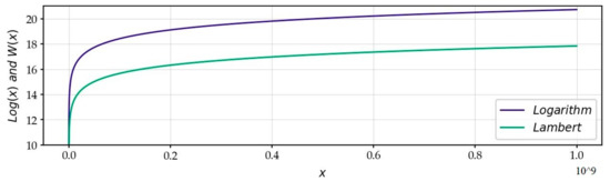
Figure 1. Comparison between the Lambert and Logarithm functions: Lambert’s function compresses high values more than the Logarithm function.

Lambert’s function enables us to examine the behavior of functions with large numbers, such as $\pi \left(x\right)$ and $Li\left(x\right)$. The Lambert function overwrites high values with a more powerful mechanism than that of the logarithm function, by abrogating the exponential component of the function: $W\left(z\right)=W\left(w{e}^w\right)=w$. In the use we are going to make of it, it will remove the exponential component $e^w$ from the function $W$, applied to $w = \ln u$: $W\left(z\right)=W\left(\ln u{e}^{\ln u}\right)=W\left(u\ln u\right)=\ln u$. In this article, it allows us to present the distribution of non-trivial zeros on the CL. Lambert’s $W$ function is the reciprocal of the complex variable function defined by $f\left(w\right)=w{e}^w$:

$$-1/e\le y<0 : -1\le W\left(y\right)<0$$

$$y\ge 0 :W\left(y\right)>0$$

$$W\left(-1/e\right)=-1; W\left(0\right)=0; W\left(e\right)=1;$$

$$W^{\prime }\left(y\right)=W\left(y\right)/\left(y\left(1+W(y\right)\right)$$

For high values of $y$: $L_1=\ln y;L_2=\ln \left(\ln y\right);W\left(y\right)=L_1-L_2+\frac{L_2}{L_1}+ O\lceil {\left(\frac{L_2}{L_1}\right)}^2\rceil$.

2.5.5. Hadamard’s Product Formula

Hadamard’s product formula contains in its expression, on the one hand, the non-trivial zeros and on the other hand, the functional Riemann equation. It therefore has a remarkable strength to characterize the zeta function and its deep relationship with neighborhoods of zeros. We know the formula:

$$\frac{{\zeta }^{\prime }\left(s\right)}{\zeta \left(s\right)}= \ln 2\pi -\raisebox{1ex}{$1$}\!\left/ \!\raisebox{-1ex}{$2$}\right.\gamma -1-\frac{1}{s-1}-\raisebox{1ex}{$1$}\!\left/ \!\raisebox{-1ex}{$2$}\right.\frac{{\mathsf{\Gamma }}^{\prime }\left(1+\raisebox{1ex}{$1$}\!\left/ \!\raisebox{-1ex}{$2$}\right.s\right)}{\mathsf{\Gamma }\left(1+\raisebox{1ex}{$1$}\!\left/ \!\raisebox{-1ex}{$2$}\right.s\right)}+{{\displaystyle \sum }}_{n=1}^{\infty }\left(\frac{1}{s-s_n}+\frac{1}{s_n}\right)$$

Moreover, we know that: ${{\displaystyle \sum }}_{n=1}^{\infty }\frac{1}{s_n}=1+ \gamma /2-\ln 2-\raisebox{1ex}{$1$}\!\left/ \!\raisebox{-1ex}{$2$}\right.\ln \pi ;\frac{{\mathsf{\Gamma }}^{\prime }\left(1+\raisebox{1ex}{$1$}\!\left/ \!\raisebox{-1ex}{$2$}\right.s\right)}{\mathsf{\Gamma }\left(1+\raisebox{1ex}{$1$}\!\left/ \!\raisebox{-1ex}{$2$}\right.s\right)}={\psi }^0\left(1+\raisebox{1ex}{$1$}\!\left/ \!\raisebox{-1ex}{$2$}\right.s\right)$

The formula becomes:

$$\frac{{\zeta }^{\prime }\left(s\right)}{\zeta \left(s\right)}= \ln \sqrt{\pi }-\raisebox{1ex}{$1$}\!\left/ \!\raisebox{-1ex}{$2$}\right.{\psi }^0\left(1+\raisebox{1ex}{$1$}\!\left/ \!\raisebox{-1ex}{$2$}\right.s\right)-\frac{1}{s-1}+{{\displaystyle \sum }}_{n=1}^{\infty }\frac{1}{s-s_n}$$

Using a CL point $𝓈$ of $ℒ$ and the zeros $\mathcal{Z}\subset ℨ$ on the CL $ℒ\subset \mathcal{S}$, which assumes the RH to be true, the infinite sum is written: ${{\displaystyle \sum }}_{n=1}^{\infty }\frac{1}{𝓈-{𝓈}_n}=-i{{\displaystyle \sum }}_{n=1}^{\infty }\frac{1}{𝓎-{𝓎}_n}$

We finally obtain, taking into account the pairs of zeros on the CL ($y>0$ and $y<0$):

$$\begin{gathered} \frac{{\zeta }^{\prime }(𝓈)}{\zeta (𝓈)} = \ln \sqrt{\pi }-\raisebox{1ex}{$1$}\!\left/ \!\raisebox{-1ex}{$2$}\right.{\psi }^0\left(1+\raisebox{1ex}{$1$}\!\left/ \!\raisebox{-1ex}{$2$}\right.𝓈\right)+\frac{1}{\overline{𝓈}}-i{{\displaystyle \sum }}_{n=1}^{\infty }\left(\frac{1}{𝓎-{𝓎}_n}+\frac{1}{𝓎+{𝓎}_n}\right) \\ =f(𝓈)+2i𝓎{{\displaystyle \sum }}_{n=1}^{\infty }\frac{1}{{𝓎}_n^2-{𝓎}^2} \end{gathered}$$

This formula converges slowly on the imaginary component, because of the terms in ${𝓎}_n^{-2}$.

When ${𝓎}_n$ is very large, we can do the approximation: ${𝓎}_n\approx \frac{2\pi \left(n-2+\raisebox{1ex}{$5$}\!\left/ \!\raisebox{-1ex}{$8$}\right.\right)}{W\left(\frac{n-2+\raisebox{1ex}{$5$}\!\left/ \!\raisebox{-1ex}{$8$}\right.}{e}\right)}\approx \frac{2\pi n}{\ln n-1}$.

The sum can then be broken down into two sums if $𝓎⋘{𝓎}_n$:

$${{\displaystyle \sum }}_{n=1}^{\infty }\frac{1}{{𝓎}_n^2-{𝓎}^2}={{\displaystyle \sum }}_{n=1}^m\frac{1}{{𝓎}_n^2-{𝓎}^2}+{{\displaystyle \sum }}_{n=m+1}^{\infty }\frac{1}{{𝓎}_n^2-{𝓎}^2}$$

We can then choose $m$ to obtain a good approximation, but the convergence is always slow.

If $𝓎$ was always very small compared to ${𝓎}_n$, which is never the case since ${𝓎}_n$ sweeps the entire range of ordinates, we could have an estimate of the infinite sum:

$$\begin{gathered} 𝓎⋘{𝓎}_n\Rightarrow {{\displaystyle \sum }}_{n=1}^{\infty }\frac{1}{{𝓎}_n^2}\approx \frac{1}{4{\pi }^2}{{\displaystyle \sum }}_{n=1}^{\infty }{\left(\frac{\ln n-1}{n}\right)}^2 \\ =\frac{1}{4{\pi }^2}\frac{{\pi }^2\left(1+2\gamma +2\ln 2\pi +{\zeta }^{″\left(2\right)}-24\ln A\right)}{6} \end{gathered}$$

$${{\displaystyle \sum }}_{n=1}^{\infty }\frac{1}{{𝓎}_n^2}\approx \frac{1}{24}\left(1+2\gamma +2\ln 2\pi +{\zeta }^{″}\left(2\right)\right)-\ln A$$

$A$ is the Glaisher–Kinkelin constant: $\ln A = \frac{1}{12}-{\zeta }^{\prime }\left(-1\right)\approx 0.2487544770337843$.

This calculation only fixes orders of magnitude for the terms ${𝓎}_n$ far from $𝓎$:

$${{\displaystyle \sum }}_{n=1}^{\infty }\frac{1}{{𝓎}_n^2}\approx {\zeta }^{\prime }\left(-1\right)+\frac{1}{24}\left(-1+2\gamma +2\ln 2\pi +{\zeta }^{″}\left(2\right)\right)=1.7591$$

2.6. The CL Zeros within the Bibliography

There are many publications on the existence and properties of the zeros of the Riemann function [18]. As early as 1896, Hadamard made subtle use of the properties of the holomorphic function. As early as 1914, authors used the powerful tools of functional analysis and Fourier transforms to deduce inequalities that led to increasingly refined results. It should be noted that in these papers, the functional Riemann equation $\zeta \left(s\right)=\xi \left(s\right)\zeta \left(1-s\right)$ is used more qualitatively for its symmetry in $s$ compared to $\left(1-s\right)$, rather than quantitatively for the value of the factor $\xi \left(s\right)$.

The main classic formulas are the following:

• Number of zeros:
  If $N\left(y\right)$ denotes the number of zeros (counting multiplicities) of $\zeta \left(s\right)=\zeta \left(x+iy\right)$ in the rectangle $ℛ:=\left\{0\le x\le 1, 0\le u\le y\right\}$, Riemann proposed the estimate $N\left(y\right)=t \ln \left(t/e\right)$, Backlund [19] obtained the specific estimate: $\left|N\left(y\right)-\left(t \ln \left(t/e\right)+\raisebox{1ex}{$7$}\!\left/ \!\raisebox{-1ex}{$8$}\right.\right)\right|<0.137\ln y+ 0.443\ln \ln y+ 4.350$.
  In 2020, the number of zeros in the rectangle is considered as

  $$N\left(y\right)=t \ln \left(t/e\right)+\raisebox{1ex}{$7$}\!\left/ \!\raisebox{-1ex}{$8$}\right.+arg\left(\zeta \left(s\right)\right)/\pi +\mathcal{O}\left(1/y\right)=t \ln \left(t/e\right)+\raisebox{1ex}{$7$}\!\left/ \!\raisebox{-1ex}{$8$}\right.+\mathcal{O}\left(1/y\right)+\mathcal{O}\left(\ln y\right)$$
  An asymptotic estimate for the zero of rank $n$, $z_n=x_n+i{y}_n$ is $\left|{𝓎}_n\right|\approx \frac{2\pi n}{\ln n}$.
• Consecutive zeros [20]:
  Assuming the RH, Feng and Wu [21] showed that the average size of the gaps is: $\forall y: \mu \left(\Delta y\right)= y_{n+1}-y_n=\frac{2\pi }{\ln y_n}$ and infinitely often: $\underset{y\in \mathbb{R}}{\min }\Delta y<0.5154 \mu \left(\Delta y\right); \underset{y\in \mathbb{R}}{\max }\Delta y>2.7327 \mu \left(\Delta y\right)$.
  Montgomery [22] suggested that there were arbitrarily large and small gaps between consecutive zeros of $\zeta \left(s\right)$, which is to say $\underset{y\in \mathbb{R}}{\min }\Delta y=0$ and $\underset{y\in \mathbb{R}}{\max }\Delta y=\infty$.
• Moment of order 2:

  $$\begin{gathered} M_2(𝓎)=\frac{1}{𝓎}{{\displaystyle \int }}_0^{𝓎}{\left|\zeta \left(\raisebox{1ex}{$1$}\!\left/ \!\raisebox{-1ex}{$2$}\right.+iu\right)\right|}^{2}du = \ln 𝓎+2\gamma -1-\ln 2\pi +\mathcal{O}\left(\ln 𝓎/\sqrt{𝓎}\right) \\ \approx \ln 𝓎-1.6834457366 \end{gathered}$$
• High moments of the Riemann zeta-function [23,24], moments of order $2k$:

  $$\forall k 2\le k\le 6, \exists C\left(k\right):M_{2k}(𝓎)={{\displaystyle \int }}_0^{𝓎}{\left|\zeta \left(\raisebox{1ex}{$1$}\!\left/ \!\raisebox{-1ex}{$2$}\right.+iu\right)\right|}^{2k}du={𝓎}^{\left(k+2\right)/4}{\left(\ln 𝓎\right)}^{C\left(k\right)} + \mathcal{O}\left({𝓎}^{\alpha }\ln {𝓎}^{\beta }\right)$$

3. Results

The results are presented in progression, over graphic illustrations, for educational purposes.

3.1. The Global Distribution Model: The Density of Zeros and the Lambert Function

Figure 2 illustrates the raw frequency of occurrence of the first 6 million zeros, adjusted to a theoretical frequency. The calculation is carried out on intervals of 200 points. The law of appearance of zeros obeys a theoretical density of probability of appearance of $1/\left(2\pi \right)\ln \left(𝓎/\left(2\pi \right)\right)$, a formula which was already known to B. Riemann.

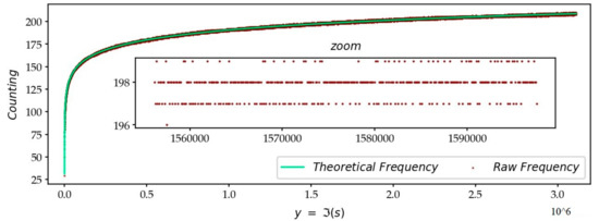
Figure 2. Density of non-trivial zeros on the CL for the first 6 million zeros. The density of the appearance of zeros, on the $y$ axis from $0$ to $3\times {10}^6$, is calculated on segments of length $200$. It is verified, on the zoom, that the experimental law remarkably follows the theoretical curve, by observing that the number of zeros in a sliding window, at this location ($1.55\times {10}^6$ to $1.6\times {10}^6$ ), ranges from 196 to 199.

Figure 3 illustrates the error between the raw density and the theoretical density.

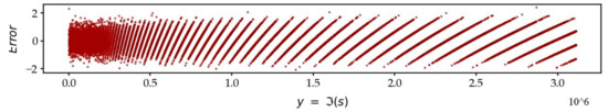
Figure 3. Error between the theoretical and experimental distribution densities. This error varies for the set $\mathcal{D}$ between $-2$ and $+2$ for segments of length $200$.

If the probability density is $1/\left(2\pi \right)\ln \left(𝓎/\left(2\pi \right)\right)$, the rank of a particular zero within the sequence $\mathcal{Z}\subset ℒ$ is $R\left({𝓎}_a\right)=n=\lceil {{\displaystyle \int }}_0^{{𝓎}_a}\ln \left(\frac{u}{2\pi }\right)d\left(\frac{u}{2\pi }\right)\rceil =\lceil \frac{𝓎}{2\pi }\ln \frac{𝓎}{2\pi e}-d\rceil =\lceil t\ln \frac{t}{e}-d\rceil$ and the number of zeros less than or equal to $𝓎$ is the integral $N\left(𝓎\right)={{\displaystyle \int }}_0^{𝓎}\ln \left(\frac{u}{2\pi }\right)d\left(\frac{u}{2\pi }\right)=t\ln \frac{t}{e}-c;c=-1+\raisebox{1ex}{$1$}\!\left/ \!\raisebox{-1ex}{$8$}\right.-\frac{arg\left(\zeta \left(𝓈\right)\right)}{\pi }; t=\frac{𝓎}{2\pi }$. We highlight here the status of the variable $t= y/\left(2\pi \right)$ of the ordinate $y$ of $𝓈=\raisebox{1ex}{$1$}\!\left/ \!\raisebox{-1ex}{$2$}\right.+iy$ which comes into play in the zeroing mechanism of the $\zeta$ function via the anamorphosed variable $\tilde{t}=t\ln \left(t/e\right)$. Thus, the Lambert $W$ function appears through the product $z\ln z$ present in the integral formula and in many formulas of the $\zeta$ function. The Lambert function thus makes it possible to exhibit the anamorphic space $\tilde{\mathbb{C}}$ by the transformation of the coordinates of $\mathbb{C}$:

$$\left\{x\to x;y\to \tilde{t}=\phi \left(y\right)=y/\left(2\pi \right)\ln \left(y/\left(2\pi e\right)\right)\iff y=2\pi e^{1+W\left(\tilde{t}/e\right)}\right\}.$$

The passage into a transformed space via this function makes it possible to simplify the study of the $\zeta$ function. After the anamorphosis of the $y$ axis, in Figure 4, we determine the constant $d= -2+\raisebox{1ex}{$5$}\!\left/ \!\raisebox{-1ex}{$8$}\right.$, by fitting the line $\tilde{t}=\varphi \left(n\right)$.

$$\tilde{t}=\phi \left(y\right)=y/\left(2\pi \right)\ln \left(y/\left(2\pi e\right)\right)=t\ln t/e=\varphi \left(n\right)=n+d=n-2+\raisebox{1ex}{$5$}\!\left/ \!\raisebox{-1ex}{$8$}\right..$$

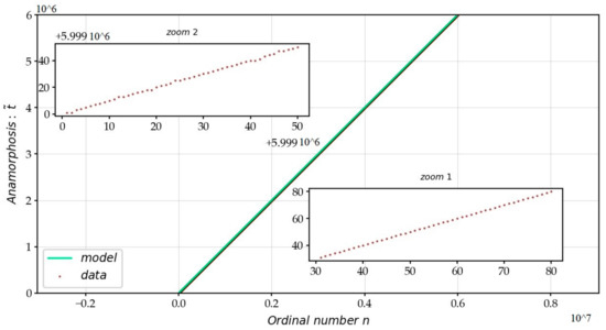
Figure 4. Curve of the first 6 million zeros after the anamorphosis of the ordinate of the $\mathbb{C}$ complex plane by the Lambert function. The adjustment of the line $\varphi \left(n\right)=n+d$ from after the anamorphosis $\tilde{t}=\phi \left(y\right)=y/\left(2\pi \right)\ln \left(y/\left(2\pi e\right)\right)$ allows us to calculate the constant $d=-2+\raisebox{1ex}{$5$}\!\left/ \!\raisebox{-1ex}{$8$}\right.$.

The value ${\tilde{t}}_n=\left[{\tilde{t}}_n\right]+\left\{{\tilde{t}}_n\right\}=n-2+r_n$ identifies the nth non-trivial zero, with $r_n\in \left[0,1\right)$ which is given a geometric interpretation below in the form of an angle. However, this formula succeeds in identifying $87\%$ of zeros but fails by $+1$ or $-1$ to qualify zeros, either ahead or behind.

In Figure 5, we represent the histogram of $\left\{\tilde{t}\right\}$ which has a maximum at ⅝ and a minimum at ⅛. We can conclude that in order to recover an integer for $R\left({𝓎}_a\right)$ more often, it is judicious to subtract ⅛ from the real value of $\tilde{t}$, in order to best estimate the integer number $R\left({𝓎}_a\right)$. Therefore, the formula $R\left({𝓎}_a\right)=n=\left[t\ln \left(t/e\right)-\raisebox{1ex}{$1$}\!\left/ \!\raisebox{-1ex}{$8$}\right.\right]+2$ is hence more correct.

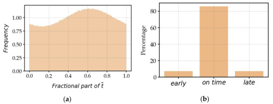
Figure 5. (a) Histogram of $\left\{\tilde{t}\right\}$ with 500 intervals: frequency minimum is at ⅛, maximum is at ⅝. We recognize a histogram made up of several random variables folded on themselves and with an average of ⅝; (b) histogram $\epsilon =R\left({𝓎}_a\right)-n$.

In Figure 6, the error on $R\left({𝓎}_a\right)=n=\lceil t\ln \frac{t}{e}-\raisebox{1ex}{$1$}\!\left/ \!\raisebox{-1ex}{$8$}\right.\rceil +2$ is $\epsilon =\pm 1$ depending on whether the nth zero is ahead ($\epsilon =-1$ with a frequency of 6.5%) or behind ($\epsilon =+1$, with a probability of 6.5%), but the error is zero in the general case (87%). We will see in the following that the maximum error increases with $n$ when $n$ is greater ($n>{10}^7$).

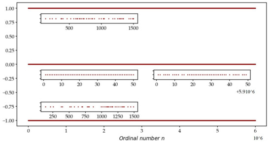
Figure 6. Error $\epsilon =R\left({𝓎}_a\right)-n=\pm 1$ versus $n$; $n\le 6\times {10}^6$.

In Table 3, we present the list of the 50 first zeros which are classified with an error of $-1$ and an error of $+1$, i.e., the list of the first zeros which are, behind and ahead, respectively.

Table 3. The 50 first early and late zero numbers.

$\mathbf{Early} \mathbf{Zero} \mathbf{Number} (\mathit{\epsilon }-\mathbf{1})$					$\mathbf{Late} \mathbf{Zero} \mathbf{Number} (\mathit{\epsilon }+\mathbf{1})$
136	705	1096	1331	1671	127	596	820	1179	1488
213	779	1113	1346	1686	196	619	849	1210	1496
256	795	1137	1404	1704	233	627	858	1251	1499
379	809	1158	1445	1746	289	655	888	1277	1514
399	871	1167	1487	1762	368	669	965	1291	1546
509	994	1209	1519	1789	380	693	996	1308	1614
531	1018	1233	1534	1798	401	716	1029	1332	1621
580	1048	1265	1545	1806	462	729	1035	1343	1647
639	1073	1296	1602	1821	519	767	1044	1431	1657
696	1088	1321	1645	1858	568	796	1114	1457	1673

When we know the ordinates of the zeros, we can therefore rectify the incorrectly estimated zeros in the formula and restore the residual which is greater than 1 in absolute value. Once this correction ${\tilde{T}}_n\to {\tilde{U}}_n={\tilde{T}}_n-\left(\pm \epsilon \right)$ has been carried out, one can calculate the new histogram which is plotted on Figure 7. One deduces the second layer of the theoretical model from it. A zero is the realization of a Gaussian random variable ${\tilde{U}}_n$. We can define the standard Gaussian variable $\tilde{V}~\mathcal{N}\left(0,1\right)$ such that: $\forall n:{\tilde{V}}_n= \frac{{\tilde{T}}_n-\left(\pm {\epsilon }_n\right)-{\mu }_n}{{\sigma }_n}$ and estimate the probability density function (PDF) which turns out to be almost a perfect Gauss Law.

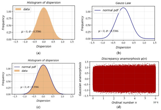
Figure 7. (a) Histogram ${\tilde{U}}_n$ with 500 intervals; (b) theoretical fit of the Gaussian curve ${\tilde{U}}_n$; (c) we check that the frequency is a perfect Gaussian curve between (a) and (b); (d) scatterplot of the deviation of ${\tilde{U}}_n$ from the mean by $n$, along $y$. This interval, which varies from $-1.5$ to $+1.5$, has extremes which deviate a little more, but in a very slow fashion, with respect to $y$.

3.2. The Local Distribution Model: the Realization of Gaussian RVs

We thus obtain a hierarchical model with two layers (Figure 8). On the $\tilde{t}= \phi \left(y\right)= \varphi \left(n\right)$ axis, we introduce ${𝓎}_{w,5}$ pivots, which will be the averages of the RVs.

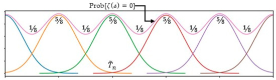
Figure 8. Stochastic process of independent Gaussian random variable (RV), regularly spaced on the $\tilde{t}$ axis. The probability of obtaining a zero is not uniform on the anamorphic $\tilde{t}$ axis: the probability is maximum for $\left\{\tilde{t}\right\}=\raisebox{1ex}{$5$}\!\left/ \!\raisebox{-1ex}{$8$}\right.$ and minimum for $\left\{\tilde{t}\right\}=\raisebox{1ex}{$1$}\!\left/ \!\raisebox{-1ex}{$8$}\right.$. The RVs overlap and the realizations of two adjacent RVs can permute: it is possible that the realization of the (n + 1)th zero precedes that of the $n\mathrm{th}$ zero.

The associated $y_n$ value with the value ${\tilde{t}}_n$ follows the realization of an associated $Y_n$ RV with the Gaussian RV ${\tilde{T}}_n$ whose average is ${\tilde{\mu }}_n=n$ and whose standard deviation ${\tilde{\sigma }}_n$ increases very slowly and is very roughly equal to $\raisebox{1ex}{$1$}\!\left/ \!\raisebox{-1ex}{$3$}\right.$ for $n<N={10}^7$. The Gaussian RVs ${\tilde{T}}_n$ are independent:

$$pdf\left({\tilde{t}}_n\right)=\frac{1}{{\tilde{\sigma }}_n\sqrt{2\pi }}{e}^{-\frac{1}{2}{\left(\frac{{\tilde{t}}_n-{\tilde{\mu }}_n}{{\tilde{\sigma }}_n}\right)}^2}$$

${\tilde{\mu }}_n=n; {\tilde{\sigma }}_n\approx 0.0462\ln \left(\ln n\right)+0.0933\ln \left(\ln \left(\ln n\right)\right)+0.122\approx 0.12555 W\left(\ln n\right)+0.08856$.

The imaginary value ${𝓎}_n$ of ${𝓈}_n=\raisebox{1ex}{$1$}\!\left/ \!\raisebox{-1ex}{$2$}\right.+ {𝓎}_n$ of the $n\mathrm{th}$ non-trivial zero is on average:

$$\forall n :{𝓎}_n^{\ast }=2\pi t_{5,n}/W\left(t_{5,n}/e\right); t_{5,n}=n-2+\raisebox{1ex}{$5$}\!\left/ \!\raisebox{-1ex}{$8$}\right..$$

The error is:$\left|{𝓎}_n-{𝓎}_n^{\ast }\right|<\frac{10}{\ln {𝓎}_n}$. See Figure 9.

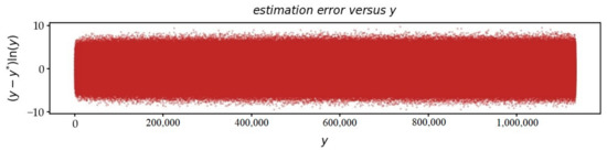
Figure 9. Scatter plot $\left({𝓎}_n-{𝓎}_n^{*}\right)ln {𝓎}_n$ versus $𝓎$. Errors become smaller and smaller as a function of $𝓎$.

Figure 10 shows a sequence of zeros, on the transformed $y$ axis, with the regularly spaced ${𝓎}_{w5}$.

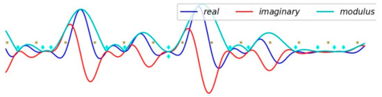
Figure 10. The 2-layer model: in the middle of the figure, two zeros ($n=4,088,664,936,218$) and $n+1$ are very close ($\Delta y=1.71\times {10}^{-5}$ ), one late, the other early, respectively. The random realization of these two zeros almost falls on $\left\{\tilde{t}\right\}=\raisebox{1ex}{$1$}\!\left/ \!\raisebox{-1ex}{$8$}\right.$, which may seem a paradox, since it is for this value ⅛, on this anamorphosed axis, that the probability of occurrence is the lowest to get a zero.

When $n$ is large, the formula becomes:

$$n\to \infty \Rightarrow {𝓎}_n\approx \frac{2\pi \left(n-2+\raisebox{1ex}{$5$}\!\left/ \!\raisebox{-1ex}{$8$}\right.\right)}{W\left(\frac{n-2+\raisebox{1ex}{$5$}\!\left/ \!\raisebox{-1ex}{$8$}\right.}{e}\right)}\approx \frac{2\pi n}{W\left(\frac{n}{e}\right)}\approx \frac{2\pi n}{\ln \frac{n}{e}-\ln \left(\ln \frac{n}{e}\right)}\approx \frac{2\pi n}{\ln n-1}\approx 2\pi \frac{n}{\ln n}$$

We undoubtedly find the similarity with the formula of the prime number theorem of Hadamard and La Vallée Poussin (1896): $\pi \left(n\right)~\frac{n}{\ln n}$.

3.3. The Heteroscedasticity of Gaussian RVs

Figure 11 shows the adjustment of the variation of the standard deviation, calculated by an estimate on a sliding neighborhood of 1000 zeros. After a rapid increase in the first values, there is a slow increase in the variance. The experimental law is: ${\tilde{\sigma }}_n=0.12555 W\left(\ln n\right)+0.08856$.

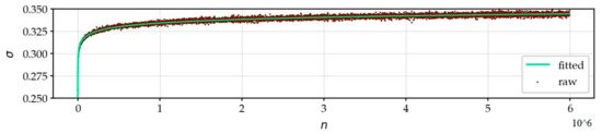
Figure 11. Adjustment of the variation of the standard deviation according to $n$.

3.4. The Equivalence Relation on the CL

The zeros of the real and imaginary parts of $\zeta (𝓈)$ are close to the pivots ${𝓎}_{w5,n}$ and ${𝓎}_{w1,n}$:

$$\forall n: \zeta \left(\raisebox{1ex}{$1$}\!\left/ \!\raisebox{-1ex}{$2$}\right.+i{𝓎}_{w5,n}\right)\approx 0+i{b}_n; \zeta \left(\raisebox{1ex}{$1$}\!\left/ \!\raisebox{-1ex}{$2$}\right.+i{𝓎}_{w1,n}\right)\approx a_n+i\times 0;a_n,b_n\in \mathbb{R}$$

$$t_{5,n}=n-2+\raisebox{1ex}{$5$}\!\left/ \!\raisebox{-1ex}{$8$}\right.; {𝓎}_{w5,n}=2\pi t_{5,n}/W\left(t_{5,n}/e\right);t_{1,n}=n-2+\raisebox{1ex}{$1$}\!\left/ \!\raisebox{-1ex}{$8$}\right.; {𝓎}_{w1,n}=2\pi t_{1,n}/W\left(t_{1,n}/e\right).$$

The alternating and regular setting to zero of the real and imaginary parts of the $\zeta$ function on the CL in the neighborhoods of the pivot values ${𝓎}_{w5,n}$ for the real part and ${𝓎}_{w1,n}$ for the imaginary part, are at the origin of the production of the nth zero of the $\zeta$ function, a zero which this time is common to both real and imaginary parts. These pivot values are not exactly the points of nullity for which a precise expression is later calculated. However, at pivotal values, there is the relation:

$$\forall n:\zeta \left(\raisebox{1ex}{$1$}\!\left/ \!\raisebox{-1ex}{$2$}\right.+i{𝓎}_{w5,n}\right)\approx a_n\left(1+i48y_{w5,n}\right)$$

$$\forall n:\zeta \left(\raisebox{1ex}{$1$}\!\left/ \!\raisebox{-1ex}{$2$}\right.+i{𝓎}_{w1,n}\right)\approx b_n\left(-48y_{w1,n}+i\right)$$

$$\left|a_n\right|,\left|b_n\right|<\epsilon , \left(\epsilon <1/n;pour n<{10}^7\right).$$

On the CL, there is a relationship between the real and imaginary parts of the $\zeta$ function:

$$\forall 𝓈=\raisebox{1ex}{$1$}\!\left/ \!\raisebox{-1ex}{$2$}\right.+i𝓎:\mathfrak{I}\left(\zeta (𝓈)\right)/\mathfrak{R}\left(\zeta (𝓈)\right)=\tan \raisebox{1ex}{$1$}\!\left/ \!\raisebox{-1ex}{$2$}\right.\omega ;\alpha =\pi /4-2\pi \left\{\tilde{t}\right\}; \theta =1/\left(24𝓎\right);\omega \approx \alpha +\theta$$

This relation (demonstrated later in Section 3.6.2) is only valid on the CL, and takes into account an angle related to the fractional part of the ordinate $\tilde{t}$, which allows us to anchor the common zeros of these two components in an equivalence relation, ${𝓎}_1\equiv {𝓎}_2\iff {\tilde{t}}_1\equiv {\tilde{t}}_2\iff \left\{{\tilde{t}}_1\right\}=\left\{{\tilde{t}}_2\right\}$:

$${𝓎}_1\equiv {𝓎}_2\iff {\alpha }_1={\alpha }_2\iff {\omega }_1\cong {\omega }_2\iff \mathfrak{I}\left(\zeta \left({𝓈}_1\right)\right)/\mathfrak{R}\left(\zeta \left({𝓈}_1\right)\right)\cong \mathfrak{I}\left(\zeta \left({𝓈}_2\right)\right)/\mathfrak{R}\left(\zeta \left({𝓈}_2\right)\right).$$

The two alternately zero $\zeta$ surfaces of period 1 on the anamorphic $\tilde{t}$ axis of the ordinate of the complex plane locally generate an additional common zero which is the nth non-trivial zero. For a non-trivial zero, the ratio becomes $0/0$, and Hospital’s rule applies in $\mathbb{C}$:

$$\mathfrak{I}\left(\zeta \left({𝓈}_1\right)\right)/\mathfrak{R}\left(\zeta \left({𝓈}_1\right)\right)=-\mathfrak{R}\left({\zeta }^{\prime }\left({𝓈}_1\right)\right)/\mathfrak{I}\left({\zeta }^{\prime }\left({𝓈}_1\right)\right)=\tan \left(\omega /2\right)$$

This equivalence relation in $\tilde{\mathbb{C}}$, where the $n$ classes are intervals ${\tilde{I}}_n$ of length 1 (Figure 12), for the segments $\forall n: {\tilde{I}}_n=\left[n-\raisebox{1ex}{$1$}\!\left/ \!\raisebox{-1ex}{$2$}\right., n+\raisebox{1ex}{$1$}\!\left/ \!\raisebox{-1ex}{$2$}\right.\right]$ characterizes the silhouettes of the $\zeta$ function on the CL, profiles which extend into the CS, and which allow us to estimate the maxima of $\left|\zeta \left(s\right)\right|$ in this CS. When one takes into account the raw values of the $y$ axis in $\mathbb{C}$, the equivalence relation is more difficult to manipulate and the underlying RVs are more convoluted. The $\tilde{\mathbb{C}}$-space distribution model removes the statistical bias caused by the strict $y$ axis support that hides the true mechanisms of the $\zeta$ function.

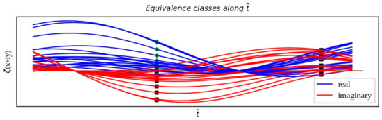
Figure 12. The equivalence relation: a few segments of the $\zeta$ curve (real and imaginary parts) along a few intervals of the anamorphic $\tilde{t}$ CL. The real (resp. imaginary) parts almost cancel each other out for the values $\tilde{t}\equiv \raisebox{1ex}{$5$}\!\left/ \!\raisebox{-1ex}{$8$}\right.$, (resp. $\raisebox{1ex}{$1$}\!\left/ \!\raisebox{-1ex}{$8$}\right.$). We almost also verified $\mathfrak{R}\left(\zeta \left(s\right)\right)=-\mathfrak{I}\left(\zeta \left(s\right)\right),$ (resp. $+\mathfrak{I}\left(\zeta \left(s\right)\right)$) for the values $\tilde{t}\equiv \raisebox{1ex}{$3$}\!\left/ \!\raisebox{-1ex}{$8$}\right., \left(resp. \raisebox{1ex}{$7$}\!\left/ \!\raisebox{-1ex}{$8$}\right.\right)$.

3.5. The Continuous Catalog of Fold Appearances of the $\zeta$ Function in the CS

The stochastic process contributes to characterizing the local $\zeta$ function landscapes. The classification of the $\zeta$ function conformations simply takes its source in the effective “random” distribution of the zeros. The key to determining taxonomy is the value of the probability density of the nearby zero (Figure 13). We can thus extract some canonical patterns, at the origin of the production of a non-trivial zero, although the catalog of these patterns constitutes a continuous spectrum. These different families of patterns show more or less regular and more or less high wave configurations, according to the standard pattern: the higher the value of the probability density of a zero is, the more regular the neighboring undulations will be; the lower the value of the probability density of a zero is, the more irregular the nearby waves will be, in particular with weak waves and a strong wave which will appear in the vicinity (Figure 14). When the probability is very low, one can identify a particular archetype consisting of a rogue wave surrounded by dead calm. More frequently, the occurrence of small distances between two consecutive zeros arises with a similar configuration of the $\zeta$ function: it is a high wave of the real part, located upstream or downstream, accompanied by wavelets of the real and the imaginary parts which graze the zero level of the plane $\mathrm{z}=0$: the corrugated sheet of both $\zeta$ surfaces in the CS also gives rise to a kind of dead calm, any homothety of the Riemann functional equation apart.

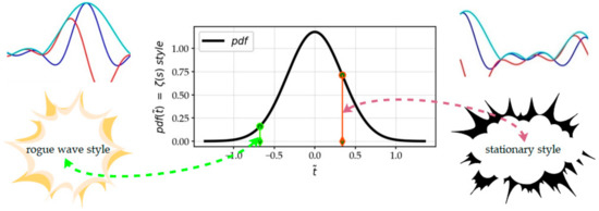
Figure 13. Classification of the local behavior styles of the zeta function according to the value of the pdf of the local zero realization. Local styles of the zeta function (real, imaginary and module) are shown: rogue wave style on the left; stationary style on the right.

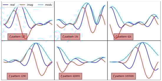
Figure 14. Six different patterns depending on the pdf of the zero linked to the segment $I_n$.

3.6. The Structural Characters of $\zeta$ and $\xi$ from the Functional Equation

In this paragraph, we develop the $\xi$ function in the power series, by taking advantage of the power series expansion of the Gamma function. This operation uses the fact that $x$ is very small compared to $y$. The calculations are geometrically interpreted in order to identify the structural features of the $\zeta$ and $\xi$ functions which are expressed by this functional equation.

In the CS, the $\xi$ function is a composition of elementary geometric functions: a homothety and four rotations ${\theta }_1+{\theta }_2+{\theta }_3+{\theta }_4$, and a series remainder function in ${\left(x-\raisebox{1ex}{$1$}\!\left/ \!\raisebox{-1ex}{$2$}\right.\right)}^2/y$:

$$\forall s\in \mathcal{S}: \zeta \left(s\right)\equiv \zeta \left(\widehat{s}\right) modulo \left(\mathcal{H}\circ {\mathcal{R}}_1\circ {\mathcal{R}}_2\circ {\mathcal{R}}_3\circ {\mathcal{R}}_4\circ \mathcal{E}\right)$$

$$\zeta \left(s\right)=\xi \left(s\right)\zeta \left(\widehat{s}\right)=t^{\raisebox{1ex}{$1$}\!\left/ \!\raisebox{-1ex}{$2$}\right.-x}{e}^{i\omega }\zeta \left(\widehat{s}\right)=t^{\raisebox{1ex}{$1$}\!\left/ \!\raisebox{-1ex}{$2$}\right.-x}{e}^{i\left({\theta }_1+{\theta }_2+{\theta }_3+{\theta }_4\right)}(1+\epsilon {(x-\raisebox{1ex}{$1$}\!\left/ \!\raisebox{-1ex}{$2$}\right.)}^2/y)\times \zeta \left(\widehat{s}\right) ; \epsilon \in \mathbb{C}$$

$$\xi \left(s\right)\times \xi \left(\widehat{s}\right)=1 \Rightarrow \left(1+\epsilon \right)\left(1+\widehat{\epsilon }\right)=1$$

The homothety is a function of $x$ and the four rotations are functions of $y$. The remainder $\left(1+\epsilon \right)$ is the only factor that mixes the two coordinates $x$ and $y$. The homothety plays its role of $\zeta$ amplification in the $0<x<\raisebox{1ex}{$1$}\!\left/ \!\raisebox{-1ex}{$2$}\right.$ region and contraction in the $\raisebox{1ex}{$1$}\!\left/ \!\raisebox{-1ex}{$2$}\right.<x<1$ region. The four rotations, two of which are pure and the other two are digressive, that is to say a little falsified, ensure the functional equation between $\zeta \left(s\right)$ and $\zeta \left(1-s\right)$.

On the CL, the homothety is neutral and only the first three rotations are effective: the $\xi$ function ensures the relation between $\zeta$ and its conjugate, via a rotation of the angle ${\theta }_1+{\theta }_2+{\theta }_3$, within an order of accuracy of ${\left(1/y\right)}^3$:

$$\forall 𝓈\in \mathcal{L}: \zeta (𝓈)\equiv \zeta (\overline{𝓈}) modulo \left({\mathcal{R}}_1\circ {\mathcal{R}}_2\circ {\mathcal{R}}_3\circ \mathcal{E}\right)$$

$$\zeta (𝓈)=\xi (𝓈)\zeta (\overline{𝓈})=e^{i\omega }\zeta (\overline{𝓈})= e^{i\left({\theta }_1+{\theta }_2+{\theta }_3\right)}(1+\epsilon {(1/y)}^3)\times \zeta (\overline{𝓈}); \epsilon \in \mathbb{C}$$

$$\xi (𝓈)\times \xi (\overline{𝓈})=1 \Rightarrow \left(1+\epsilon \right)\left(1+\overline{\epsilon }\right)=1$$

3.6.1. The Functional Equation in the CS

The functional relationship is written:

$$s=x+iy; \widehat{s}=1-s; \zeta \left(s\right)=\xi \left(s\right)\zeta \left(\widehat{s}\right) ; \xi \left(s\right)={\pi }^{s-\raisebox{1ex}{$1$}\!\left/ \!\raisebox{-1ex}{$2$}\right.}\frac{\mathsf{\Gamma }\left(\widehat{s}/2\right)}{\mathsf{\Gamma }\left(s/2\right)}; \xi \left(s\right)\xi \left(\widehat{s}\right)=1$$

The power series of the Gamma function is:

$$\mathsf{\Gamma }\left(z\right)=\sqrt{2\pi }{z}^{z-\raisebox{1ex}{$1$}\!\left/ \!\raisebox{-1ex}{$2$}\right.}{e}^{-z+\mu \left(z\right)} pour z\in \mathbb{C}\backslash {\mathbb{Z}}_{-};\mu \left(z\right)={\displaystyle {\sum }_{k=1}^{\infty }}\frac{{\mathcal{B}}_{2k}}{2k\left(2k-1\right)z^{2k-1}}$$

${\mathcal{B}}_i$ are the Bernoulli numbers.

In the CS, we can then develop the $\xi$ function in series, assuming $0<x<1⋘y$:

$$t= y/\left(2\pi \right); \tilde{t}=t\ln \left(t/e\right); {\theta }_1=\pi /4; {\theta }_2=-2\pi \left\{\tilde{t}\right\}; {\theta }_3=-1/\left(24y\right); {\theta }_4=-{\left(x-\raisebox{1ex}{$1$}\!\left/ \!\raisebox{-1ex}{$2$}\right.\right)}^2/\left(2y\right);$$

$$\alpha ={\theta }_1+{\theta }_2=2\pi \left(\raisebox{1ex}{$1$}\!\left/ \!\raisebox{-1ex}{$8$}\right.-\left\{\tilde{t}\right\}\right); \omega \approx {\theta }_1+{\theta }_2+{\theta }_3+{\theta }_4$$

$$\xi \left(s\right)=t^{\raisebox{1ex}{$1$}\!\left/ \!\raisebox{-1ex}{$2$}\right.-x}{e}^{i\omega }=t^{\raisebox{1ex}{$1$}\!\left/ \!\raisebox{-1ex}{$2$}\right.-x}{e}^{i\alpha } \mathcal{A}\left(s\right)=t^{\raisebox{1ex}{$1$}\!\left/ \!\raisebox{-1ex}{$2$}\right.-x}{e}^{i\left({\theta }_1+{\theta }_2\right)}\left(e^{i\left({\theta }_3+{\theta }_4\right)}+\mathcal{K}\left(s\right)\right)=t^{\raisebox{1ex}{$1$}\!\left/ \!\raisebox{-1ex}{$2$}\right.-x}{e}^{i\left({\theta }_1+{\theta }_2\right)} e^{i\left(\breve{{\theta }_3+{\theta }_4}\right)}$$

$$\begin{gathered} \mathcal{K}\left(s\right)=-2i{\theta }_4+\frac{{\theta }_3}{2y}\left(x-\raisebox{1ex}{$1$}\!\left/ \!\raisebox{-1ex}{$2$}\right.\right)\left(1-10x+8x^2\right) \\ -\frac{i{\theta }_3}{y^2}\left(-\frac{7}{120}+\left(x-\raisebox{1ex}{$1$}\!\left/ \!\raisebox{-1ex}{$2$}\right.\right)\left(-\frac{5}{24}-\raisebox{1ex}{$1$}\!\left/ \!\raisebox{-1ex}{$2$}\right.x+\frac{23x^2}{12}-\raisebox{1ex}{$1$}\!\left/ \!\raisebox{-1ex}{$2$}\right.x^3+\raisebox{1ex}{$1$}\!\left/ \!\raisebox{-1ex}{$2$}\right.x^4-x^5\right)\right) \\ +\frac{{\theta }_3^2}{ y^2}\left(-\frac{7}{120}+\left(x-\raisebox{1ex}{$1$}\!\left/ \!\raisebox{-1ex}{$2$}\right.\right)\left(\frac{133}{720}+\frac{2753x}{360}+\frac{707x^2}{60}-\frac{181x^3}{10}-\frac{87x^4}{10}-5x^5+12x^6\right)\right)+\cdots \end{gathered}$$

When the point $s$ is on the CL, the expression is simplified:

$$\mathcal{K}(𝓈)=\mathcal{K}\left(\raisebox{1ex}{$1$}\!\left/ \!\raisebox{-1ex}{$2$}\right.+i𝓎\right)=i\frac{168}{5}{\theta }_3^3\left(1+{\theta }_3+\cdots \right); {\theta }_3=-1/\left(24y\right)$$

The serial expansion of $\xi \left(s\right)=t^{\raisebox{1ex}{$1$}\!\left/ \!\raisebox{-1ex}{$2$}\right.-x}{e}^{i\left({\theta }_1+{\theta }_2\right)}\left(e^{i\left({\theta }_3+{\theta }_4\right)}+\mathcal{K}\left(s\right)\right)$ is interpreted as a function composed of a homothety $t^{\raisebox{1ex}{$1$}\!\left/ \!\raisebox{-1ex}{$2$}\right.-x}$ and four rotations, the first two being pure rotations.

• The homothety supports the $n^{-x}$ effect of the power of the $n^{-s}$ terms of the $\zeta$ function, with the symmetry at $x=\raisebox{1ex}{$1$}\!\left/ \!\raisebox{-1ex}{$2$}\right.$. The CL is a neutral element of the homothety.
• The rotation $\mathcal{R}\left({\theta }_1=\pi /4\right)$ comes from the offset of the real surface which is, in probability, above the imaginary surface, due to the imbalance of the first term of the series of $\left(\cos \left(y\ln 1\right)=1;\sin \left(y\ln 1\right)=0\right)$. This rotation restores, on average, the two surfaces to the same level.
• The major rotation $\mathcal{R}\left({\theta }_2=-2\pi \left\{\tilde{t}\right\}=-2\pi \left\{t\ln \left(t/e\right)\right\}\right)$ erases the sinuousness of the $\xi$ function. This rotation, dependent on $y$, shears by continuous torsions, in order to make the undulations disappear.
• The rotation $\mathcal{R}\left({\theta }_3=-1/\left(24y\right)\right)$ is numerically and graphically barely perceptible. It is impure because the series contains higher order terms which alter the rotation. This rotation has a decisive influence in the genesis of the zeros of the two surfaces, and consequently in the materialization of non-trivial zeros.
• The impure rotation $\mathcal{R}\left({\theta }_4=-{\left(x-\raisebox{1ex}{$1$}\!\left/ \!\raisebox{-1ex}{$2$}\right.\right)}^2/\left(2y\right)\right)$ is not perceptible on the CL. It has an intrinsic role in the CS, because it is the impurity of this digressive rotation which breaks the symmetry at the level of each term of the series in $1/y$ and which does not make it possible to manufacture the two pairs of zeros ($s,\widehat{s} and \overline{s}, \widehat{\overline{s}}$) outside the CL (for $y>$ and $y<0$).

The third and fourth rotations are impure (or digressive) rotations: the symmetry in $x$ and $1-x$ is thus not respected by the series $\mathcal{K}\left(s\right)$ from the term in $1/y^2$ in the CS, except on the CL, which geometrically explains the RH.

3.6.2. The Functional Equation on the CL

In this paragraph, we show, using the properties of the functional equation, that the real and imaginary curves of the $\zeta$ function regularly and alternately cancel each other out, thanks to $\xi (𝓈)$ which nearly instantiates in two perfect sinusoids on the CL. It is this alternation that generates a non-trivial zero in a restricted interval. On the CL, the calculations are extremely simplified:

$$𝓈=\raisebox{1ex}{$1$}\!\left/ \!\raisebox{-1ex}{$2$}\right.+i𝓎; \zeta (𝓈)=\xi (𝓈)\zeta (\widehat{𝓈})=\xi (𝓈)\zeta (\overline{𝓈})=\xi (𝓈)\overline{\zeta (𝓈)}\Rightarrow \left|\xi (𝓈)\right|=1\Rightarrow \xi (𝓈)=e^{i\omega }$$

$$\xi (𝓈)={\pi }^{i𝓎}\frac{\mathsf{\Gamma }(\widehat{𝓈}/2)}{\mathsf{\Gamma }\left(𝓈/2\right)}={\pi }^{i𝓎}\frac{\overline{\mathsf{\Gamma }\left(𝓈/2\right)}}{\mathsf{\Gamma }\left(𝓈/2\right)}; \xi (𝓈)\overline{\xi (𝓈)}=1$$

By multiplying by $\zeta (𝓈)$ if $𝓈$ is not a zero: ${\left(\zeta (𝓈)\right)}^2= \xi (𝓈)\overline{\zeta (𝓈)}\zeta (𝓈)=\xi (𝓈){\left|\zeta (𝓈)\right|}^2$

$$\left|\zeta (𝓈)\right|\ne 0 \Rightarrow \xi (𝓈)={\left(\frac{\zeta (𝓈)}{\left|\zeta (𝓈)\right|}\right)}^2=e^{i\omega } \Rightarrow \zeta (𝓈)= \pm \left|\zeta (𝓈)\right|e^{i\omega /2}\Rightarrow \frac{\mathfrak{I}\left(\zeta (𝓈)\right)}{\mathfrak{R}\left(\zeta (𝓈)\right)}=\tan \frac{\omega }{2}$$

If ${𝓈}_n$ is zero, Hospital’s rule gives: ${\left({\zeta }^{\prime }\left({𝓈}_n\right)\right)}^2=-\xi \left({𝓈}_n\right){\left|{\zeta }^{\prime }\left({𝓈}_n\right)\right|}^2$

$$\left|\zeta (𝓈)\right|=0 \Rightarrow \xi (𝓈)=-{\left(\frac{{\zeta }^{\prime }\left({𝓈}_n\right)}{\left|{\zeta }^{\prime }\left({𝓈}_n\right)\right|}\right)}^2=e^{i\omega } \Rightarrow {\zeta }^{\prime (𝓈)}= \pm i\left|{\zeta }^{\prime (𝓈)}\right|e^{i\omega /2}\Rightarrow -\frac{\mathfrak{R}\left({\zeta }^{\prime }(𝓈)\right)}{\mathfrak{I}\left({\zeta }^{\prime }(𝓈)\right)}=\tan \frac{\omega }{2}$$

The non-trivial zeros are at the breaking point of the two functions $+e^{i\omega /2}$ and $-e^{i\omega /2}$.

Using the power series expansion of $\mathsf{\Gamma }\left(𝓈/2\right)$, we serially expand $\xi (𝓈)$ to find $\omega$:

$$\left|\xi (𝓈)\right|=1\Rightarrow \xi (𝓈)=e^{i\omega }=e^{i\left(\alpha +\beta \right)} ; \alpha =\pi /4-2\pi \left\{\tilde{t}\right\}; \theta =-1/\left(24𝓎\right);$$

$$e^{i\beta }=\left(1-\frac{3\mathrm{i}}{8𝓎}-\frac{9}{128{𝓎}^2}+\frac{139\mathrm{i}}{3072{𝓎}^3}+\frac{475}{32768{𝓎}^4}+\cdots \right)\left(1+\frac{\mathrm{i}}{3𝓎}-\frac{1}{18{𝓎}^2}-\frac{73\mathrm{i}}{1620{𝓎}^3}+\frac{131}{9720{𝓎}^4}+\cdots \right)$$

$$\begin{gathered} e^{i\beta }=\breve{e^{i\theta }}=1-\frac{\mathrm{i}}{24𝓎}-\frac{1}{2!{\left(24𝓎\right)}^2}-\frac{\left(6\times 7\times 24-5\right)\mathrm{i}}{5\times 3!{\left(24𝓎\right)}^3}-\frac{7\times {24}^2-5}{5\times 4!{\left(24𝓎\right)}^4}-\frac{19\times 31\times 8707\mathrm{i}}{7\times 5!{\left(24𝓎\right)}^5}-\frac{317\times 531103}{35\times 6!{\left(24𝓎\right)}^6} \\ -\frac{13\times 5243712823\mathrm{i}}{5\times 7!{\left(24𝓎\right)}^7}-\frac{31\times 661\times 28660561}{5\times 8!{\left(24𝓎\right)}^8}-\frac{27\times 8197117457520809\mathrm{i}}{25\times 11\times 9!{\left(24𝓎\right)}^9} \\ -\frac{81\times 5099\times 4517050132181}{11\times 5\times 10!{\left(24𝓎\right)}^{10}}+\cdots \end{gathered}$$

We can therefore extract the rotation ${\theta }_3=\theta =-1/\left(24y\right)$ from this expansion: $e^{i\beta }=e^{i\theta }+{\mathcal{P}}_3\left(i\theta \right)$

$$\beta =arg\left(e^{i\theta }+{\mathcal{P}}_3\left(i\theta \right)\right)\approx \theta =-1/\left(24𝓎\right)$$

${\mathcal{P}}_3$ is a three-order polynomial in $i\theta =-i/\left(4!𝓎\right)$:

$$\begin{gathered} {\mathcal{P}}_3=\frac{24{\theta }^3}{5}\left(7i-7\theta +i\frac{17807}{7\times 2!}{\theta }^2-\frac{29\times 10079}{7\times 5\times 3!}{\theta }^3+i\frac{43\times 11009087}{7\times 5\times 4!}{\theta }^4-\frac{{13}^{2}131\times 23027}{7\times 5!}{\theta }^5 \\ +i\frac{3458158927391587}{3\times 5\times 7\times 9\times 11\times 6!}{\theta }^6-\frac{7\times 47\times 2095343\times 148000093}{3\times 5\times 7\times 9\times 11\times 7!}{\theta }^7+\cdots \right) \end{gathered}$$

$$\begin{gathered} e^{i\beta }=e^{i\theta }\left(1+i\frac{168}{5}{\theta }^3\right) \\ +\frac{4i{\theta }^5}{35}\left(31\times {12}^3+\frac{36}{5}\left(34\times 239i\theta +2\times 1643717{\theta }^2+53\times 66797i{\theta }^3\right) \\ +\frac{1}{{45}^{2}11}\left(68\times 61\times 107923\times 965611{\theta }^4+23\times 4881469\times 16227313i{\theta }^5\right)+\cdots \right). \end{gathered}$$

We can deduce an approximate value of $\xi (𝓈)$ on the CL:

$${𝒫}_3\approx i\frac{168}{5}{\theta }^3\left(1+i\theta \right); \theta =-1/\left(24𝓎\right)$$

$$\xi (𝓈)=e^{i\omega }\approx e^{i\alpha }\left(e^{i\theta }+i\frac{168}{5}{\theta }^3\left(1+i\theta \right)\right)\approx e^{i\left(\alpha +\theta \right)}\left(1+i\frac{168{\theta }^3}{5}\right)\approx e^{i\left(\alpha +\theta +\frac{168{\theta }^3}{5}\right)}\approx e^{i\left(\alpha +\theta \right)}$$

The functional equation on the CL does not represent a pure rotation, but this equation allows to define an equivalence relation, within the order of ${\mathcal{R}}_3\circ \mathcal{E}$. With this equivalence relation, the CL is a concatenation of equivalence class instantiations of unit length along the anamorphic axis $\tilde{t}$.

$$\forall {𝓈}_1, {𝓈}_2\in \mathcal{L}: {𝓈}_1\equiv {𝓈}_2\iff \left\{{\tilde{t}}_1\right\}\equiv \left\{{\tilde{t}}_2\right\}\iff \xi \left({𝓈}_1\right)=\xi \left({𝓈}_2\right) modulo \left({\mathcal{R}}_3\circ \mathcal{E}\right)\iff aspect \zeta \left({𝓈}_1\right)\equiv aspect \zeta \left({𝓈}_2\right)$$

Now, we will be able to determine the alternating zeros of the real and imaginary curves, by taking advantage of this evaluation via an approximate calculation of the derivative.

3.6.3. The Zeros of the Real and Imaginary Parts of the $\zeta$ Function

In this paragraph, we perform the calculations assuming the approximation: $\omega ={\theta }_1+{\theta }_2+{\theta }_3+{\theta }_4$.

On the CL, we can calculate the derivative of $\xi (𝓈)$ at constant $x$, as a function of $y$:

$$\omega = \pi /4-2\pi \left\{\tilde{t}\right\}+\theta \Rightarrow {\omega }^{\prime }=-\ln t+1/\left(4!{𝓎}^2\right)=-\ln t-\theta /𝓈; \theta ={\theta }_3=-1/\left(24𝓎\right)$$

$${\xi }^{\prime }(𝓈)={\left(e^{i\omega }\right)}^{\prime }=i{\omega }^{\prime }{e}^{i\omega }=i{e}^{i\omega }\left(-\ln t+1/\left(4!{𝓎}^2\right)\right)$$

The values of $𝓎$ for which $\zeta (𝓈)$ cancel each other out for the real part (resp. the imaginary part), correspond to the values for which $\xi (𝓈)=-1$ (resp. $\xi (𝓈)=1$). They coincide with the values close to $\left\{\tilde{t}\right\}=\raisebox{1ex}{$5$}\!\left/ \!\raisebox{-1ex}{$8$}\right.$ (resp. $\left\{\tilde{t}\right\}=\raisebox{1ex}{$1$}\!\left/ \!\raisebox{-1ex}{$8$}\right.$), that is to say the values $\alpha =\pi$, (resp. $\alpha =0$).

We assume in the calculations: $\omega = \alpha +\theta =\pi /4-2\pi \left\{𝓎/\left(2\pi \right)\ln \left(𝓎/\left(2\pi e\right)\right)\right\}-1/\left(24𝓎\right)$.

$$\zeta (𝓈)=\xi (𝓈)\zeta (\overline{𝓈}); \zeta (𝓈)=𝒶+𝒾𝒷; 𝒶+𝒾𝒷=e^{i\omega }\left(𝒶-𝒾𝒷\right); \xi (𝓈)=𝒸+𝒾𝒹;$$

Case where$\left\{\tilde{t}\right\}=\raisebox{1ex}{$1$}\!\left/ \!\raisebox{-1ex}{$8$}\right.;$

$$\begin{gathered} \alpha =0 ; \xi (𝓈)=e^{i\omega }=e^{i\beta }\approx e^{i\theta }= e^{-i/\left(4!𝓎\right)}\approx 1-\frac{i}{24𝓎}-\frac{1}{1152{𝓎}^2}+\cdots \\ 𝒶+𝒾𝒷={𝓮}^{𝒾\beta }\left(𝒶-𝒾𝒷\right) \\ 𝒶\left(1-{𝓮}^{𝒾\beta }\right)+𝒾𝒷\left(1+{𝓮}^{𝒾\beta }\right)=0\Rightarrow 𝒶\sin \left(\beta /2\right)=𝒷\cos \left(\beta /2\right); 𝒷/𝒶=\tan \left(\beta /2\right)\approx -\tan \left(1/\left(48𝓎\right)\right) \\ 𝒸=1-\epsilon ; 𝒹=-ϵ \\ {𝒸}^2+ {𝒹}^2=1 \Rightarrow 𝒷/𝒶=-\epsilon /ϵ;{\epsilon }^2-2\epsilon +{ϵ}^2=0 \Rightarrow \epsilon \approx {ϵ}^2/2 \Rightarrow 𝒷/𝒶= 𝒹/2 \end{gathered}$$

It follows then that: $\xi (𝓈)\approx 1-{𝒹}^2/2+𝒾𝒹=1-1/\left(1152{𝓎}^2\right)-𝒾/\left(24𝓎\right); 𝒷/𝒶=d/2\approx -1/\left(48𝓎\right)$

To improve the estimation of ${𝓎}_{1,n}$ such that $\zeta (𝓈)=\zeta \left(\raisebox{1ex}{$1$}\!\left/ \!\raisebox{-1ex}{$2$}\right.+i{𝓎}_{1,n}\right)=𝒶+𝒾𝒷=𝒶$, we must take into account the derivative of $\xi$. Hence, we can calculate the difference $\mathsf{\Delta }𝓎$ with the pivot value ${𝓎}_{n,w1}$:

$$\mathsf{\Delta }𝓎=\frac{\theta }{{\omega }^{\prime }}=\frac{-1/\left(24𝓎\right)}{-\ln t+1/\left(4!{𝓎}^2\right)}={\left(24𝓎\ln \frac{𝓎}{2\pi }-\frac{1}{𝓎}\right)}^{-1}$$

The approximate value of $𝓎$ for which $\zeta (𝓈)$ has a null imaginary value is therefore:

$$\begin{gathered} \zeta \left(\raisebox{1ex}{$1$}\!\left/ \!\raisebox{-1ex}{$2$}\right.+𝒾{𝓎}_{1,n}\right)={𝒶}_n+𝒾 0\Rightarrow {𝓎}_{1,n}={𝓎}_{w1,n}+\mathsf{\Delta }𝓎 \\ {t}_{1,n}=n-2+\raisebox{1ex}{$1$}\!\left/ \!\raisebox{-1ex}{$8$}\right.; {𝓎}_{w1,n}=2\pi t_{1,n}/W\left(t_{1,n}/e\right);t_{w1,n}={𝓎}_{w1,n}/\left(2\pi \right) \\ 𝓎\approx {𝓎}_{w1,n}+1/\left(4!{𝓎}_{w1,n}\ln t_{w1,n}-1/{𝓎}_{w1,n}\right) \\ \forall n\in \mathbb{N}: \zeta (𝓈)=\zeta \left(\raisebox{1ex}{$1$}\!\left/ \!\raisebox{-1ex}{$2$}\right.+𝒾{𝓎}_{1,n}\right)={𝒶}_n\Rightarrow \xi (𝓈)=1 ;{𝓎}_{1,n}\approx {𝓎}_{w1,n}+1/\left(4!{𝓎}_{w1,n}\ln t_{w1,n}-1/{𝓎}_{w1,n}\right) \end{gathered}$$

Case where$\left\{\tilde{t}\right\}=\raisebox{1ex}{$5$}\!\left/ \!\raisebox{-1ex}{$8$}\right.;$

$$\begin{gathered} \alpha =\pi ; \xi (𝓈)=e^{i\omega }=e^{i\left(\pi +\beta \right)}=-e^{i\beta }\approx -e^{i\theta }= -e^{-i/\left(4!y\right)}\approx -\left(1-\frac{i}{24𝓎}-\frac{1}{1152{𝓎}^2}+\cdots \right) \\ 𝒶+𝒾𝒷=e^{i\omega }\left(𝒶-𝒾𝒷\right)=-{𝓮}^{𝒾\beta }\left(𝒶-𝒾𝒷\right) \\ 𝒶\left(1+{𝓮}^{𝒾\beta }\right)+𝒾𝒷\left(1-{𝓮}^{𝒾\beta }\right)=0\Rightarrow 𝒶\cos \left(\beta /2\right)=𝒷\sin \left(\beta /2\right); 𝒶/𝒷=\tan \left(\beta /2\right)\approx \tan \left(1/\left(48𝓎\right)\right) \\ 𝒸=-1+\epsilon ; 𝒹=ϵ \\ 𝒶/𝒷=\epsilon /ϵ;{\epsilon }^2-2\epsilon +{ϵ}^2=0 \Rightarrow \epsilon ={ϵ}^2/2 \Rightarrow 𝒶/𝒷= 𝒹/2 \end{gathered}$$

It follows then that: $$\begin{gathered} \xi (𝓈)\approx -1+{𝒹}^2/2+𝒾𝒹=-1+1/\left(1152{𝓎}^2\right)+𝒾/\left(24𝓎\right); 𝒶/𝒷=d/2\approx 1/\left(48𝓎\right) \\ {t}_{5,n}=n-2+\raisebox{1ex}{$5$}\!\left/ \!\raisebox{-1ex}{$8$}\right.; {𝓎}_{w5,n}=2\pi t_{5,n}/W\left(t_{5,n}/e\right);t_{w5,n}={𝓎}_{w5,n}/\left(2\pi \right) \\ \forall n\in \mathbb{N}: \zeta (𝓈)=\zeta \left(\raisebox{1ex}{$1$}\!\left/ \!\raisebox{-1ex}{$2$}\right.+𝒾{𝓎}_{5,n}\right)=𝒾{𝒷}_n\Rightarrow \xi (𝓈)=-1 ;{𝓎}_{5,n}\approx {𝓎}_{w5,n}+1/\left(4!y_{w5,n}\ln t_{w5,n}-1/{𝓎}_{w5,n}\right) \end{gathered}$$

Case where$\left\{\tilde{t}\right\}=\raisebox{1ex}{$3$}\!\left/ \!\raisebox{-1ex}{$8$}\right.;$

$$\begin{gathered} \alpha =-\pi /2; \xi (𝓈)=e^{i\omega }=e^{i\left(-\pi /2+\beta \right)}=-i{e}^{i\beta }\approx -i{e}^{i\theta }= -i{e}^{-i/\left(4!𝓎\right)}\approx -i-\frac{1}{24𝓎}+\frac{i}{1152{𝓎}^2}+\cdots \\ 𝒶+𝒾𝒷=e^{i\omega }\left(𝒶-𝒾𝒷\right)=-i{𝓮}^{𝒾\beta }\left(𝒶-i𝒷\right) \end{gathered}$$

It follows that: $$\begin{gathered} \xi (𝓈)\approx c-i\left(1-c^2/2\right)=\theta -i\left(1-{\theta }^2/2\right)=-1/\left(24𝓎\right)-i+i/\left(1152{𝓎}^2\right); a\approx -b \\ {t}_{3,n}=n-2+\raisebox{1ex}{$3$}\!\left/ \!\raisebox{-1ex}{$8$}\right.; y_{w3,n}=2\pi t_{3,n}/W\left(t_{3,n}/e\right);t_{w3,n}=y_{w3,n}/\left(2\pi \right) \\ \forall n\in \mathbb{N}: \zeta (𝓈)=\zeta \left(\raisebox{1ex}{$1$}\!\left/ \!\raisebox{-1ex}{$2$}\right.+𝒾{𝓎}_{3,n}\right)={𝒶}_n\left(1-i\right)\Rightarrow \xi (𝓈)=-i ;{𝓎}_{3,n}\approx {𝓎}_{w3,n}+1/\left(4!{𝓎}_{w3,n}\ln t_{w3,n}-1/{𝓎}_{w3,n}\right) \end{gathered}$$

Case where$\left\{\tilde{t}\right\}=\raisebox{1ex}{$7$}\!\left/ \!\raisebox{-1ex}{$8$}\right.;$

$$\begin{gathered} \alpha =\pi /2; \xi (𝓈)=e^{i\omega }=e^{i\left(\pi /2+\beta \right)}=i{e}^{i\beta }\approx i{e}^{i\theta }= i{e}^{-i/\left(4!𝓎\right)}\approx i+\frac{1}{24𝓎}+\frac{-i}{1152{𝓎}^2}+\cdots ; \\ 𝒶+𝒾𝒷=e^{i\omega }\left(𝒶-𝒾𝒷\right)=i{𝓮}^{𝒾\beta }\left(𝒶-𝒾𝒷\right) \end{gathered}$$

It follows that: $$\begin{gathered} \xi (𝓈)\approx 𝓈+i\left(1-{𝒸}^2/2\right)=-\theta +i\left(1-{\theta }^2/2\right)=1/\left(24𝓎\right)+i-i/\left(1152{𝓎}^2\right); a\approx b \\ {t}_{7,n}=n-2+\raisebox{1ex}{$7$}\!\left/ \!\raisebox{-1ex}{$8$}\right.; {𝓎}_{w7,n}=2\pi t_{7,n}/W\left(t_{7,n}/e\right);t_{w7,n}={𝓎}_{w7,n}/\left(2\pi \right) \\ \forall n\in \mathbb{N}: \zeta (𝓈)=\zeta \left(\raisebox{1ex}{$1$}\!\left/ \!\raisebox{-1ex}{$2$}\right.+𝒾{𝓎}_{7,n}\right)={𝒶}_n\left(1+i\right)\Rightarrow \xi (𝓈)=i ;{𝓎}_{7,n}\approx {𝓎}_{w7,n}+1/\left(4!{𝓎}_{w7,n}\ln t_{w7,n}-1/{𝓎}_{w7,n}\right) \end{gathered}$$

3.7. The Consecutive Zeros on the CL

Figure 15a shows the rather asymmetrical histogram of the raw distances between two consecutive zeros from $\mathcal{D}$. The tail of the histogram has not been represented for values greater than $1.5$: these are some large differences of the first zeros ($𝓎<\mathrm{50,000}$). Figure 15b represents the scatterplot of these distances along the $𝓎$ ordinate. We observe that these distances, on average, tend to decrease with $𝓎$, and we understand from this figure that the raw $𝓎$ axis is not the most appropriate variable to study the statistics of gaps between zeros. It is preferable to analyze the population of the gaps between zeros, after anamorphosis, along the $\tilde{t}$ axis.

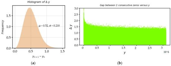
Figure 15. (a) Histogram of the gaps between two consecutive zeros, calculated on the raw $y$ axis, $y>\mathrm{500,000}$. Indeed, the first $\Delta y$ is an outlier at 6.887; (b) the scatterplot of the gaps between two zeros as a function of the $y$ ordinate.

Figure 16a,b show the graphs, after the transformation of the $y$ axis into the $\tilde{t}$ axis. We greatly reduced the influence of the bias of the use of the variable $𝓎$. There is only a slight asymmetry, which can be interpreted as follows. We selected the zeros in the order of appearance on the $𝓎$ axis, so that the difference between ${𝓎}_{n+1}$ and ${𝓎}_n$ is always positive, as is the difference $\mathrm{\Delta }{\tilde{t}}_n={\tilde{t}}_{n+1}-{\tilde{t}}_n$. It goes without saying that there are possible underlying permutations between the indices $n$ and $n+1$. If there was a way to identify these permutations of indices of consecutive zeros, especially when the zeros are relatively close, the gaps between some adjacent zeros could be negative, and in this case, the left part of the histogram would have a branch which would overflow towards negative values, still with mean 1. We would then obtain a much more symmetrical and Gaussian histogram.

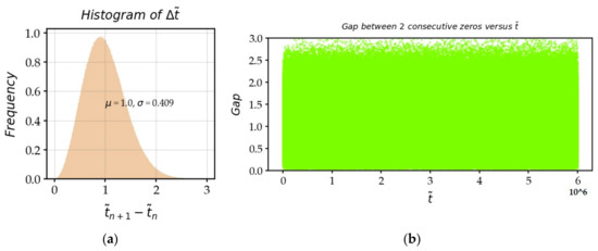
Figure 16. (a) Histogram of the gaps between two consecutive zeros calculated on the anamorphic $\tilde{t}$ axis; and (b) scatterplot of the gaps between two zeros as a function of the anamorphic ordinate $\tilde{t}$.

The model expresses it clearly. The difference between two independent mixed RVs ${\tilde{T}}_{n+1}$ and ${\tilde{T}}_n$ is a new Gaussian RV $\mathrm{\Delta }{\tilde{T}}_n=\mathcal{N}\left({\tilde{\mu }}_{\mathsf{\Delta }},{\tilde{\sigma }}_{\mathsf{\Delta }n}\right)$ of parameters ${\tilde{\mu }}_{\mathsf{\Delta }}={\tilde{\mu }}_{n+1}- {\tilde{\mu }}_n=\left(n+1\right)-n=1; {\tilde{\sigma }}_{\mathsf{\Delta }n}={\tilde{\sigma }}_n$. We can calculate the average distance between two consecutive zeros $\mathsf{\Delta }{y}_n=y_{n+1}-y_n$:

$$\forall n :\mathsf{\Delta }{\mu }_n={\mu }_{n+1}-{\mu }_n=\frac{2\pi t_{5,n+1}}{W\left(t_{5,n+1}/e\right)}-\frac{2\pi t_{5,n}}{W\left(t_{5,n}/e\right)}\approx \frac{2\pi }{W\left(t_{5,n}/e\right)}; t_{5,n}=n-2+\raisebox{1ex}{$5$}\!\left/ \!\raisebox{-1ex}{$8$}\right..$$

$$\forall n :\mathsf{\Delta }{y}_n\approx \frac{2\pi }{W\left(\left(n-2+\raisebox{1ex}{$5$}\!\left/ \!\raisebox{-1ex}{$8$}\right.\right)/e\right)}\approx \frac{2\pi }{\ln \left(y_n/\left(2\pi e\right)\right)};\mathsf{\Delta }{t}_n\times \ln \left(t_n/e\right)\approx 1;t_n=\frac{y_n}{2\pi }$$

We can get, for $N<{10}^7$, an estimation of the drift of extreme values of $\mathsf{\Delta }y$ as a function of $y$:

$$\forall 𝓎: \frac{2\pi /200}{\ln \left(y/2\pi e\right)}=\frac{0.01\pi }{\ln \left(y/2\pi e\right)}<\mathsf{\Delta }y<\frac{2\pi \times 2\times 4.5\sigma }{\ln \left(y/2\pi e\right)}=\frac{6\pi }{\ln \left(y/2\pi e\right)}$$

The passage from $y$ to $\tilde{t}$ makes it possible to better compare the differences in the list of non-trivial zeros from $\mathcal{D}$: some adjacent zeros are very close or far apart from each other (Figure 17).

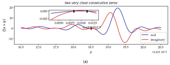
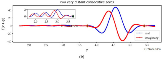
Figure 17. Two very close zeros (a) and two very distant zeros (b). On the CL, the curves $\zeta \left(\mathcal{s}\right)$ have configurations where the undulations are very weak, in the vicinity of a very large fold.

This is the case, without being exhaustive, in Table 4, for the following pairs of zeros.

Table 4. (a) List of near consecutive zeros; and (b) the list of distant consecutive zeros.

(a) The Smallest Gaps between Zeros				(b) The Biggest Gaps between Zeros
$\mathit{n}$	$\mathbf{\Delta }{\tilde{\mathit{t}}}_{\mathit{n}}$	${\mathit{y}}_{\mathit{n}}$	$\mathbf{\Delta }{\mathit{y}}_{\mathit{n}}$	$\mathit{n}$	$\mathbf{\Delta }{\tilde{\mathit{t}}}_{\mathit{n}}$	${\mathit{y}}_{\mathit{n}}$	$\mathbf{\Delta }{\mathit{y}}_{\mathit{n}}$
1,115,578	0.0054468	663,318.508	0.002959	3,206,674	3.3637376	1,746,643.719	1.686
5,042,995	0.0061228	2,650,984.611	0.002970	1,493,008	3.3034734	865,897.915	1.754
3,637,897	0.0065627	1,961,773.993	0.003259	1,793,281	3.2257130	1,024,176.503	1.689
3,271,858	0.0083140	1,779,292.804	0.004161	1,663,325	3.2221292	955,946.684	1.697
3,966,813	0.0083818	2,124,605.420	0.004137	2,865,881	3.2146956	1,575,130.462	1.625
420,891	0.0096951	273,193.663	0.005704	880,694	3.2142617	534,572.843	1.780
4,156,678	0.0098793	2,218,149.333	0.004859	5,640,489	3.2016993	2,939,651.982	1.541
4,980,819	0.0100586	2,620,810.352	0.004884	3,867,228	3.1954605	2,075,412.008	1.580
4,398,867	0.0111705	2,337,027.805	0.005472	5,491,901	3.1935420	2,868,076.402	1.540
1,205,484	0.0117584	712,004.001	0.006348	4,847,419	3.1773669	2,555,978.540	1.546

3.8. The Multiplicity of Zeros

It follows from the numerical value of the standard deviation of the Gaussian RVs that the multiplicity of zeros is achievable thanks to the constant mixing of the close RVs and that the possibility of this configuration increases with the value of $n$. It could be at the maximum of order 3 when $n<{10}^7$: it would then be necessary that the $\left(n-1\right)$th zero arrives late, the $n$th arrives in advance, and that in addition, the $\left(n+1\right)$th also occurs very early. This scenario never appears in the first few million zeros and its probability is also very low:

$$\mathbb{P}rob\{{\tilde{t}}_n+\raisebox{1ex}{$1$}\!\left/ \!\raisebox{-1ex}{$8$}\right.<\{{\tilde{T}}_{n-1}\},\{{\tilde{T}}_n\},\{{\tilde{T}}_{n+1}\}<{\tilde{t}}_n+\raisebox{1ex}{$1$}\!\left/ \!\raisebox{-1ex}{$8$}\right.+\Delta \tilde{t}\}=p$$

$$p=p_1{p}_2{p}_3\Delta {\tilde{t}}^3={0.396}^2\times 0.645\times {10}^{-4}{\left(1/2\pi \ln \left(y/2\pi \right)\Delta y\right)}^3\approx {10}^{-5}{\left(1/2\pi \ln \left(y/2\pi \right)\Delta y\right)}^3;$$

$$y= {10}^7; \Delta y= {10}^{-3}:p\approx 1.2\times {10}^{-15}.$$

The possibility of a double root is more likely, although it is known that, among the trillion zeros calculated, no double roots have yet been identified. The probability is $p=p_1{p}_2\Delta {\tilde{t}}^2\approx 8\times {10}^{-9}$, for $y= {10}^7; \Delta y= {10}^{-4}$, knowing that the nearest zeros on $\mathcal{D}$ are distant from $\Delta y\approx 0.003$. We know [15] that between the $n^{\mathrm{th}}=\mathrm{4,088,664,936,218}$ and the (n + 1)th, the gap is $\Delta y\approx 0.00001710$. Notwithstanding, the probability ($p={10}^{-9}$) for this rare event is “quite large”.

Hadamard’s product formula, dynamically interpreted via geometric analysis, provides a better understanding of the possibility of the multiple root phenomenon. We know that if ${𝓈}_p$ is a simple root $\zeta \left({𝓈}_p\right)=0$, ${\zeta }^{\prime }\left({𝓈}_p\right)=\pm i\left|{\zeta }^{\prime }\left({𝓈}_p\right)\right|e^{i\omega /2}$ is not null. Both members of Hadamard’s formula equilibrate by the term $1/\left({𝓈}_p-{𝓈}_p\right)=\infty$, present in the second member:

$$\frac{{\zeta }^{\prime }\left({𝓈}_p\right)}{\zeta \left({𝓈}_p\right)}=\frac{\pm i\left|{\zeta }^{\prime }\left({𝓈}_p\right)\right|e^{i\omega /2}}{0}=f\left({𝓈}_p\right)+\frac{1}{0}+2i{𝓎}_p{{\displaystyle \sum }}_{n=1,n\ne p}^{\infty }\frac{1}{{𝓎}_n^2-{𝓎}_p^2}$$

We study, below, the configuration of the $\zeta$ function when two zeros are very close. We know that when the real part (resp. the imaginary part) of the derivative of $\zeta$ is null, the imaginary part (resp. the real part) of the $\zeta$ function is located on a local extremum:

$\mathfrak{R}\left({\zeta }^{\prime }\left(𝓈\right)\right)=0 \Rightarrow \mathfrak{I}\left(\zeta \left(𝓈\right)\right)$ on a local extremum for the $\zeta$ curve on the $x=\raisebox{1ex}{$1$}\!\left/ \!\raisebox{-1ex}{$2$}\right.$ axis.

$\mathfrak{I}\left({\zeta }^{\prime }\left(𝓈\right)\right)=0 \Rightarrow \mathfrak{R}\left(\zeta \left(𝓈\right)\right)$ on a local extremum for the $\zeta$ curve on the $x=\raisebox{1ex}{$1$}\!\left/ \!\raisebox{-1ex}{$2$}\right.$ axis.

We observe on the graphs (Figure 18), that for a double root to exist, it would be necessary that $\zeta$ (both real and imaginary parts) be tangent to the CL $x=\raisebox{1ex}{$1$}\!\left/ \!\raisebox{-1ex}{$2$}\right.$. We would then be dealing with an extremum (local maximum or minimum) of the function for the two curves. We would therefore have in this case $\zeta \left(𝓈\right)={\zeta }^{\prime }\left(𝓈\right)=0$. If there is such a double root, the behavior of the two members of Hadamard’s formula is changed. In the rest of this paragraph, it is no longer assumed that the zeros are all on the CL. We recall that if $s\in ℨ$ is a zero of the CS, then $\widehat{s}=1-s, \overline{s}, 1-\overline{s}$ are also zeros. Now, we examine the geometric configuration of two different zeros belonging to two neighboring quartets if they are both in the CS, in two pairs if they are both on the CL, or in a quartet and a duet if they are one in the CS and the other on the CL.

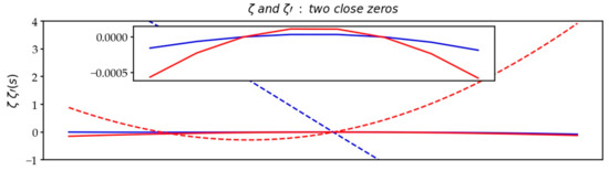
Figure 18. Plot for two near zeros: $\zeta$ function (solid lines) and ${\zeta }^{\prime }$ derivative (dotted lines).

It is assumed that the points $R_m$ and $R_{m+1}$ of indices $m$ and $m+1$ are roots with very close coordinates $s_m$ and $s_{m+1}$. We choose the point $O$ with coordinates $s$ in the middle of the segment $R_m{R}_{m+1}$: $s=\raisebox{1ex}{$1$}\!\left/ \!\raisebox{-1ex}{$2$}\right.\left(s_m+s_{m+1}\right)$. The Hadamard formula applied to point $O$ becomes:

$$\frac{{\zeta }^{\prime }\left(s\right)}{\zeta \left(s\right)}= \ln \sqrt{\pi }-\raisebox{1ex}{$1$}\!\left/ \!\raisebox{-1ex}{$2$}\right.{\psi }^0\left(1+\raisebox{1ex}{$1$}\!\left/ \!\raisebox{-1ex}{$2$}\right.s\right)-\frac{1}{s-1}+\frac{1}{s-s_m}+\frac{1}{s-s_{m+1}}+{{\displaystyle \sum }}_{n=1;n\ne m, m+1}^{\infty }\frac{1}{s-s_n};$$

$${\psi }^0\left(1+\raisebox{1ex}{$1$}\!\left/ \!\raisebox{-1ex}{$2$}\right.s\right)=\frac{ {\mathsf{\Gamma }}^{\prime }\left(1+\raisebox{1ex}{$1$}\!\left/ \!\raisebox{-1ex}{$2$}\right.s\right)}{\mathsf{\Gamma }\left(1+\raisebox{1ex}{$1$}\!\left/ \!\raisebox{-1ex}{$2$}\right.s\right)}$$

$O$ being the middle, we obtain: $\frac{1}{s-s_m}+\frac{1}{s-s_{m+1}}=0$. The second member becomes a function of $s$ which takes finite real and imaginary values of $\mathbb{C}$:

$$\ln \sqrt{\pi }-\raisebox{1ex}{$1$}\!\left/ \!\raisebox{-1ex}{$2$}\right.{\psi }^0\left(1+\raisebox{1ex}{$1$}\!\left/ \!\raisebox{-1ex}{$2$}\right.s\right)-\frac{1}{s-1}+{{\displaystyle \sum }}_{n=1;n\ne m, m+1}^{\infty }\frac{1}{s-s_n}=f\left(s\right)\in \mathbb{C}\backslash \{\infty \}$$

The $\zeta$ function is holomorphic; we can write at point $O$:

$$\zeta \left(s\right)= \zeta \left(s_m\right)+\frac{\Delta s}{1!}{\zeta }^{\prime }\left(s_m\right)+\frac{{\left(\Delta s\right)}^2}{2!}{\zeta }^{″}\left(s_m\right)+\cdots ; \Delta s=s-s_m$$

The derived function is holomorphic; we can write at point $O$:

$${\zeta }^{\prime }\left(s\right)= {\zeta }^{\prime }\left(s_m\right)+\frac{\Delta s}{1!}{\zeta }^{″}\left(s_m\right)+\frac{{\left(\Delta s\right)}^2}{2!}{\zeta }^{‴}\left(s_m\right)+\cdots$$

In the configuration of close zeros, $\zeta \left(s_m\right)=0$ and ${\zeta }^{\prime }\left(s_m\right)=\epsilon \cong {\epsilon }_1+i{\epsilon }_2$. It follows that:

$$\frac{{\zeta }^{\prime }\left(s\right)}{\zeta \left(s\right)}=\frac{{\epsilon }_1+i{\epsilon }_2+\Delta s\times {\zeta }^{″}\left(s_m\right)+\cdots }{\Delta s\times \left({\epsilon }_1+i{\epsilon }_2\right)+\raisebox{1ex}{$1$}\!\left/ \!\raisebox{-1ex}{$2$}\right.{\left(\Delta s\right)}^2\times {\zeta }^{″}\left(s_m\right)+\cdots }=\frac{1}{\Delta s}\left(\frac{{\epsilon }_1+i{\epsilon }_2+\Delta s\times {\zeta }^{″}\left(s_m\right)+\cdots }{{\epsilon }_1+i{\epsilon }_2+\raisebox{1ex}{$1$}\!\left/ \!\raisebox{-1ex}{$2$}\right.\Delta s\times {\zeta }^{″}\left(s_m\right)+\cdots }\right)$$

$$\frac{{\zeta }^{\prime }\left(s\right)}{\zeta \left(s\right)}\approx \frac{1}{\Delta s}\left(1+\frac{\raisebox{1ex}{$1$}\!\left/ \!\raisebox{-1ex}{$2$}\right.\Delta s\left({\zeta }^{″}\left(s_m\right)+\Delta s\times {\zeta }^{‴}\left(s_m\right)\right)+\cdots }{{\epsilon }_1+i{\epsilon }_2+\raisebox{1ex}{$1$}\!\left/ \!\raisebox{-1ex}{$2$}\right.\Delta s\times {\zeta }^{″}\left(s_m\right)+\raisebox{1ex}{$1$}\!\left/ \!\raisebox{-1ex}{$6$}\right.{\left(\Delta s\right)}^2{\zeta }^{‴}\left(s_m\right)+\cdots }\right)\approx \frac{2}{\Delta s}$$

When $s_m$ and $s_{m+1}$ converge, the midpoint $s$ also converges and we obtain:

$$\Delta s\to 0;{\epsilon }_1\to 0; {\epsilon }_2\to 0; \Rightarrow \frac{{\zeta }^{\prime }\left(s\right)}{\zeta \left(s\right)}\approx \frac{2}{\Delta s}\to \infty \left(\in \mathbb{C}{{\displaystyle \cup }}^{ }\{\infty \}\right)$$

It goes without saying that if ${\zeta }^{″}\left(s_m\right)=0$, we extend the expansion until we find a non-zero derivative ${\zeta }^{\left(k\right)}\left(s_m\right)\ne 0$, which is always feasible since the $\zeta$ function is not uniformly null. In conclusion, the first member takes an infinite complex value, while the second member is finite, which justifies that the double root configuration is impossible. The holomorphic property that is included in Taylor’s formula accounts for the neighborhood very close to zero. It is essentially the analysis of the local extrema of the $\zeta$ function in relation to the behavior of the derivative, i.e., the observation of the zeros of the derivative of the real and imaginary parts that triggers the justification.

3.9. The Approximation Formulas of the Extremes of $\zeta$ and of the kth Order Moments on the CL

By efficiently using the relation $\mathfrak{I}\left(\zeta \left(𝓈\right)\right)/\mathfrak{R}\left(\zeta \left(𝓈\right)\right)=\tan \left(\omega /2\right)$, it is easier to numerically estimate the curves of the $\zeta$ maxima on the CL, and to derive results from them in the CS. In addition, the $\zeta$ maxima, being rare events, it is advisable to carry out a $\pi /4$ rotation of the $\zeta$ function, in order to make the three surfaces (real, imaginary and modulus) of the function be at the same level, and to make the estimation of extremes more robust. The regular sampling of the $\zeta$ function from $\left\{\tilde{t}\right\}/8$, and not a regular sampling from $𝓎$, also allows us to calculate with better accuracy the kth-order moments of the $\zeta$ function. We find the following formulas from the sample data:

$$\begin{gathered} \forall n\in \left[1, 2\times {10}^6\right];k\in \left[1,8\right]: \zeta \left(𝓈\right);𝓈=\raisebox{1ex}{$1$}\!\left/ \!\raisebox{-1ex}{$2$}\right.+i{𝓎}_{n,w,k} \\ =\raisebox{1ex}{$1$}\!\left/ \!\raisebox{-1ex}{$2$}\right.+i2\pi \left(n-2+k/8\right)/W\left(\left(n-2+k/8\right)/e\right) \end{gathered}$$

$$M_0\left(𝓎\right)=\underset{u<y}{\max }\left|\zeta \left(\raisebox{1ex}{$1$}\!\left/ \!\raisebox{-1ex}{$2$}\right.+iu\right)\right|=\underset{u<y}{\max }\left|\mathfrak{R}\left(e^{i\pi /4}\zeta \left(\raisebox{1ex}{$1$}\!\left/ \!\raisebox{-1ex}{$2$}\right.+iu\right)\right)\right|=\underset{u<y}{\max }\left|\mathfrak{I}\left(e^{i\pi /4}\zeta \left(\raisebox{1ex}{$1$}\!\left/ \!\raisebox{-1ex}{$2$}\right.+iu\right)\right)\right|$$

Figure 19 shows the fitting of the maxima modulus of the zeta function:

$$M_0\left(𝓎\right)\approx 2.865 {𝓎}^{0.195}\approx 0.921\left({𝓎}^{0.128}{\left(\ln 𝓎 \right)}^{0.786}\right)$$

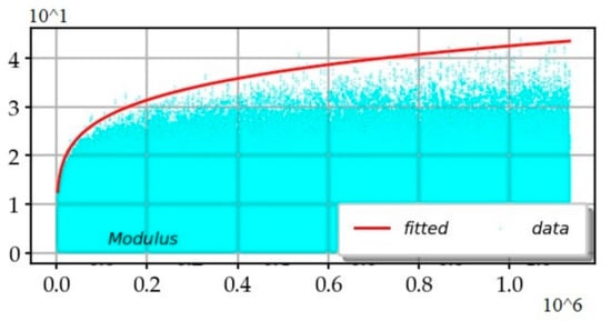
Figure 19. Adjusted curve (in red) of the maximum of the modulus of the zeta function and data (in cyan) of the moduli of the $8\times 1.2\times {10}^6$ values of the zeta moduli.

• Order 1 moment: $M_1\left(𝓎\right)=\frac{1}{𝓎}{{\displaystyle \int }}_0^{𝓎}\left|\zeta \left(\raisebox{1ex}{$1$}\!\left/ \!\raisebox{-1ex}{$2$}\right.+iu\right)\right|du\approx -0.00661\ln 𝓎 + 0.694\ln \ln 𝓎 +0.357$
• Order 2 moment: $M_2\left(𝓎\right)=\frac{1}{𝓎}{{\displaystyle \int }}_0^{𝓎}{\left|\zeta \left(\raisebox{1ex}{$1$}\!\left/ \!\raisebox{-1ex}{$2$}\right.+iu\right)\right|}^{2}du\approx \ln 𝓎 +2\gamma -1-\ln 2\pi \approx \ln 𝓎 -1.6834$
• Order 3 moment: $M_3\left(𝓎\right)=\frac{1}{𝓎}{{\displaystyle \int }}_0^{𝓎}{\left|\zeta \left(\raisebox{1ex}{$1$}\!\left/ \!\raisebox{-1ex}{$2$}\right.+iu\right)\right|}^{3}du\approx \frac{0.86375}{2{\pi }^2}{\left(\ln 𝓎\right)}^3+ 16.53$
• Order 4 moment: $M_4\left(𝓎\right)=\frac{1}{𝓎}{{\displaystyle \int }}_0^{𝓎}{\left|\zeta \left(\raisebox{1ex}{$1$}\!\left/ \!\raisebox{-1ex}{$2$}\right.+iu\right)\right|}^{4}du\approx 1/\left(2{\pi }^2\right){\left(\ln 𝓎 \right)}^4+0.123{\left(\ln 𝓎 \right)}^3-0.748{\left(\ln 𝓎 \right)}^2+1.402\ln 𝓎 -0.816$.

Table 5 shows the estimations for higher even moments from 6 to 12.

Table 5. $M_{2k}\left(𝓎\right)={{\displaystyle \int }}_0^{𝓎}{\left|\zeta \left(\raisebox{1ex}{$1$}\!\left/ \!\raisebox{-1ex}{$2$}\right.+iu\right)\right|}^{2k}du={𝓎}^{\left(k+2\right)/4}\left(A\left(k\right){\left(\ln 𝓎 \right)}^{C\left(k\right)}+B\left(k\right)\right)$ for $k=3$ to 6.

k	2k	(k + 2)/4	${\mathit{M}}_{2\mathit{k}}$	C(k)	A(k)	B(k)
3	6	5/4	$M_6$	4	0.67	−1040
4	8	3/2	$M_8$	4.62	3.34	−26,600
5	10	7/4	$M_{10}$	5.42	11	−640,300
6	12	2	$M_{12}$	6.40	26	−15,184,200

Figure 20 shows the fitting of the first power moments. $M_0\left(𝓎\right)$ and the numerical values of the coefficients $C\left(k\right)$ for the higher moments are significant for the Lindelöf conjecture which is equivalent to the statement: $\frac{1}{𝓎}{{\displaystyle \int }}_0^{𝓎}{\left|\zeta \left(\raisebox{1ex}{$1$}\!\left/ \!\raisebox{-1ex}{$2$}\right.+iu\right)\right|}^{2k}du=\mathcal{O}\left({𝓎}^{\epsilon }\right) \forall k\in \mathbb{N},\forall \epsilon >0$.

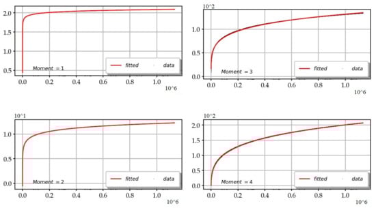
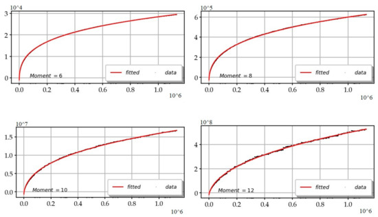
Figure 20. Raw curves and theoretical fittings of the moments $M_1, M_2, M_3, M_4, M_6, M_8, M_{10}, M_{12}$.

4. Discussion

4.1. The Rank (Position) of a Particular Zero and the Number of Zeros below a Threshold $y$

On the distribution of zeros, the model answers two distinct questions:

• Finding the rank (position) $R\left({𝓎}_a\right)=n$ of a particular zero in the sequence $\mathcal{Z}\subset ℒ$. Knowing a zero on the CL, what is the estimate of the order number $n$ of this zero? After processing the set $\mathcal{D}$ of the first zeros, we found a law in order to estimate the rank of zero in the ordered sequence $\mathcal{Z}≔\{{𝓎}_1<{𝓎}_2<\cdots < {𝓎}_n<\cdots \}$: $R^{*}\left({𝓎}_a\right)=n=\left[t \ln t/e-\raisebox{1ex}{$1$}\!\left/ \!\raisebox{-1ex}{$8$}\right.\right]+2;n=a\pm 1$.
• Finding $N\left(𝓎\right)=n$. Given a value $𝓎\in \mathbb{R}$, what is the number $N\left(𝓎\right)$ of zeros less than $𝓎$? The answer to this classic question on the Riemann function requires, according to the traditional formula, to compute the argument of $\zeta \left(𝓈\right)=𝒶+i𝒷; N^{*}\left(𝓎\right)=t \ln \left(t/e\right)+\raisebox{1ex}{$7$}\!\left/ \!\raisebox{-1ex}{$8$}\right.+ arg\left(\zeta \left(s\right)\right)/\pi$.

This complementary term $arg\left(\zeta \left(𝓈\right)\right)/\pi$ is easy to explain thanks to the model (Figure 21). Indeed, the argument (the phase of the complex number), on the transformed CL, is a sawtooth function, piecewise quasi-linear, whose value $\raisebox{1ex}{$1$}\!\left/ \!\raisebox{-1ex}{$2$}\right.\omega$ has been calculated by the model to the nearest $\pi$, and whose indeterminacy can be removed if we obtain $sign\left(𝒶\right),sign\left(𝒷\right)$, the signs of $\zeta \left(𝓈\right)$. The almost linear aspect is within $\left\{\tilde{t}\right\}$. On a $\left\{\tilde{t}\right\}$ interval of length 1, starting at ⅛, the argument is almost zero (in fact, $arg\left(\zeta \left(\raisebox{1ex}{$1$}\!\left/ \!\raisebox{-1ex}{$2$}\right.+i{𝓎}_{w1,n}\right)\right)={\tan }^{-1}\left(1/48{𝓎}_{w1,n}\right) modulo \pi$), then decreases, then goes back up by a jump of $<1$ when a new zero is emerging, and finally decreases in order to rejoin the $0$ value. On this unit segment, there is the probable appearance of a new zero and the complementary term thus increases by 1. The break $\pm e^{i\raisebox{1ex}{$1$}\!\left/ \!\raisebox{-1ex}{$2$}\right.\omega }$ and the jump take place at the location of a non-trivial zero, hence the formula for the number of zeros $N\left(𝓎\right)$. Unfortunately, there is sometimes an untimely earlier or later stall when the probability on a non-trivial zero is low and this zero is then far from the mean and outside the interval $\left[\left\{\tilde{t}\right\}=\raisebox{1ex}{$1$}\!\left/ \!\raisebox{-1ex}{$8$}\right.,\left\{\tilde{t}\right\}+1 \right]$. Therefore, $arg\left(\zeta \left(𝓈\right)\right)$ cannot account for this eccentric stall and there is then a local error on the estimated $N\left(𝓎\right)$ value. This situation happens around the following first zeros: $213,233,289,368,379,380,399,401,462,509,519,568,580,596,619,627,639,655,$ $669,693,696,705,716,729,767,795,796,809,820,849,858,871,888,965,996$.

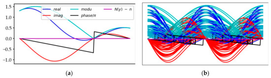
Figure 21. (a) A segment $I_n$ of $\left\{\tilde{t}\right\}$ starting at ⅛ showing the break of the term $arg\left(\zeta \left(s\right)\right)/\pi$ at the zero location; (b) 50 plots of $\left\{\tilde{t}\right\}$: we observe the properties of 2 adjacent equivalence classes.

The similarity between both general formulas therefore appears:

$$R^{*}\left({𝓎}_a\right)=\left[t \ln t/e-\raisebox{1ex}{$1$}\!\left/ \!\raisebox{-1ex}{$8$}\right.\right]+1+1;N^{*}\left(𝓎\right)=t \ln \left(t/e\right)-\raisebox{1ex}{$1$}\!\left/ \!\raisebox{-1ex}{$8$}\right.+1+ arg\left(\zeta \left(s\right)\right)/\pi$$

Knowing $\raisebox{1ex}{$1$}\!\left/ \!\raisebox{-1ex}{$2$}\right.\omega =\raisebox{1ex}{$1$}\!\left/ \!\raisebox{-1ex}{$2$}\right.\left(\alpha +\theta \right)=\pi /8-\pi \left\{t \ln \left(t/e\right)\right\}-1/\left(96\pi t\right)$ which is only dependent of $𝓎=2\pi t$ and knowing in which quadrant is located $\left(a,b\right)$, we can infer the last term $arg\left(\zeta \left(s\right)\right)/\pi$:

$$1st,4th quadrant:\omega /2\pi ;2nd quadrant:\omega /2\pi +1 ;3rd quadrant:-\omega /2\pi -\raisebox{1ex}{$1$}\!\left/ \!\raisebox{-1ex}{$2$}\right..$$

4.2. Heteroscedasticity and the Evolution of the Hierarchical Model According to $n$

The RVs ${\tilde{T}}_n$ are uniformly distributed along the axis $\tilde{t}$, of mathematical expectation ${\tilde{\mu }}_n=n$, and of slowly increasing standard deviation:

$${\tilde{\sigma }}_n=0.12555 W\left(\ln n\right)+0.08856$$

with for small $n$: $\forall n< N={10}^7: 0.23<{\tilde{\sigma }}_n<0.346$.

The difference between the minimum and maximum probability densities is of the order of:

$$\tilde{t}\left(pd{f}_{max}\right)-\tilde{t}\left(pd{f}_{min}\right)<2\left(0.033 \ln \left(n\right)+0.7 \pm 0.2\right).$$

The Gaussian RV ${\tilde{T}}_n$ is experimentally truncated at $k\tilde{\sigma }$: $\forall n<{10}^7: {\tilde{Y}}_n\in \left[n-k\tilde{\sigma }, n+k\tilde{\sigma }\right];k\approx 4;8\tilde{\sigma }<2.77$. For $n<N, N\cong {10}^{20}$, the numerical value of the standard deviation $\tilde{\sigma }$ on the transformed axis $\tilde{t}$ allows the overlapping of two consecutive RVs on each interval ${\tilde{I}}_n=\left[n-\raisebox{1ex}{$1$}\!\left/ \!\raisebox{-1ex}{$2$}\right., n+\raisebox{1ex}{$1$}\!\left/ \!\raisebox{-1ex}{$2$}\right.\right]$. Thus, with the extension to $8\tilde{\sigma }$ in $\tilde{\mathbb{C}}$ of the RV ${\tilde{T}}_n$, the RVs ${\tilde{T}}_n$ and ${\tilde{T}}_{n+1}$ overlap and some realizations of two consecutive RVs are switched. The $n^{th}$ zero can lie in one of the three intervals ${\tilde{I}}_{n-1},{\tilde{I}}_n,{\tilde{I}}_{n+1}$. Therefore, it is possible that zeros can be ahead (in the interval ${\tilde{I}}_{n-1}$, in $6.5\%$ of cases), that zeros are late (in the interval ${\tilde{I}}_{n+1}$ in $6.5\%$ of case), but in general ($87\%$ of cases) the zeros are “on time” in the interval ${\tilde{I}}_n=\left[{\mu }_n-k\sigma , {\mu }_n+k\sigma \right];k\cong 1.5$.

With such standard deviations for the RV, it often happens, including for small $n$ (for example $n=136$), that both the (n − 1)th and nth zeros or the nth and (n + 1)th zeros are in the same interval ${\tilde{I}}_n$. The model then facilitates the calculation of the number of zeros less than a value $𝓎$ with a possible error of $-1, 0, +1$. In this distribution model, the RVs ${\tilde{T}}_n$ are considered as independent. It is thus possible (and this happens theoretically in $1.84\%$ of cases for $n<N$) that the RV ${\tilde{T}}_{n+1}$ is located before the RV ${\tilde{T}}_n$. Thus, the (n + 1)th zero attached to RV ${\tilde{T}}_{n+1}$ arrives ahead and the nth zero attached to the RV ${\tilde{T}}_n$ arrives late, so much so that a permutation in the arrival orders, to which the zeros in question are linked, is possible. With this assumption of independence of RVs ${\tilde{T}}_n$, the (n + 1)th zero attached to the RV ${\tilde{T}}_{n+1}$ is in fact the nth according to the order of arrival on the $𝓎$ axis. However, this assumption of independence does not identify where these permutations take place. Knowledge should be extracted from an additional phenomenon, resulting from the morphogenesis of the $\zeta$ function, in order to pinpoint the permutations. In the absence of additional knowledge of the mechanism which produces zeros, we can avoid the obstacle of permutations in the arrival order, and be satisfied by considering a simpler interpretation: the RVs are Gaussian and all pairwise independent, except two successive Gaussian RVs ${\tilde{T}}_n$ and ${\tilde{T}}_{n+1}$, which are dependent with the constraint ${\tilde{T}}_n<{\tilde{T}}_{n+1}$. With this parameterization, the order $n$ of arrival is always compatible with the number of the RV $Y_n$.

When $n$ is very large $n>N;N\approx {10}^{100}$, the Gaussian RV spreads more widely, so that the mixing of RVs becomes more and more frequent. The $n$th zero might lie within the interval of $\left[n-2, n+2\right]$ zeros, and we would need to consider more than two consecutive RVs to be greater or smaller than the value of the previous RV. Any permutations are then more challenging to interpret.

4.3. The Limits of the Model

It is crucial to determine the limits of a theoretical model. The current model was inferred from values of $y<{10}^{20}$. We cannot claim to generalize this model beyond this value without making some hypotheses or assumptions which must be justified. If the model seems robust in its architecture, we can discuss the legitimacy of the use of the full normal distribution, the independence of adjacent RVs and the heteroscedasticity of the sequence of normal laws, which proceeds from a more fragile induction. Calculations towards $N={10}^{100}$ on a segment $\Delta n={10}^{10}$ are essential to finally being able to confirm these properties.

4.3.1. Questioning the Legitimacy of Statistics: Observation versus Genesis

The second layer of the model implements RVs. However, the origin of zeros is concealed under experimental observation through a statistical filter. Needless to say, the successive zeros of the CL do not obey the morphogenetic assumptions of a random distribution, since the $\zeta$ function is deterministic. The occurrence of a zero is generated by the nullity coincidence of both members of the infinite sum of trigonometric functions $e^{-i\left(y \ln n modulo 2\pi \right)}/\sqrt{n}$, and this simultaneity is not due to chance. The Laplace–Gauss law is one of the foundations of statistics, based on the law of large numbers summarizing the work of Laplace [25], Čebyšëv [26] and Paul Lévy [27]. Statistics which focus more on the analysis of the RV’s average behavior, rather than on rare events, should be used with caution when considering the extremes of mathematical functions. RVs are assumed to be independent, but the local layout is no accident (Figure 22). The Poisson model [28], which is the basis for the analysis of series of independent observations, is therefore not a suitable model for the appearance of zeros, because of the undeniable local dependence of the various sub-series of adjacent zeros.

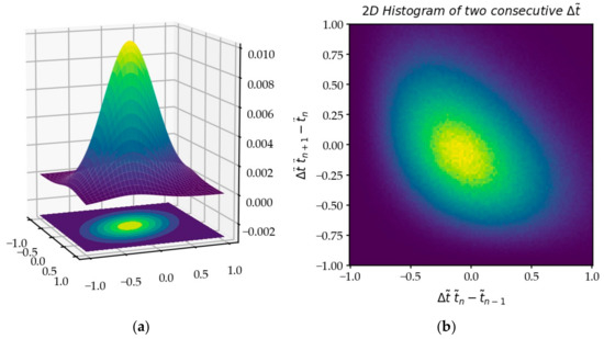
Figure 22. (a) Gaussian 2D distribution; (b) the 2D histogram of successive increments is not fully a Gaussian distribution (see the upper right part): $Y_n$ and $Y_{n+1}$ are dependent: $Y_n<Y_{n+1}$.

If we accept the systematic dependence of two successive RVs $Y_n<Y_{n+1}$, the process can even be considered as Markovian since: $\mathbb{P}\left(Y_{n+1}\right|Y_n,\dots ,Y_1)=\mathbb{P}(Y_{n+1}\left|Y_n\right)$, with the constraint $y_{n+1}>y_n$.

4.3.2. Questioning a Normal Distribution or a Normal Distribution Truncated to $\pm \mathrm{k}\mathsf{\sigma }$

If the use of a normal distribution over an infinite interval is improper, then the normal distribution must be reduced to a truncated Gaussian distribution ${\mathcal{N}}_T\left({\tilde{\mu }}_n,{\tilde{\sigma }}_n^2{\sigma }^2,k\left(n\right)\right)$, again is it necessary to determine the value of the coefficient $k$ of the maximum spacing $\left[{\tilde{\mu }}_n-k{\tilde{\sigma }}_n,{\tilde{\mu }}_n+k{\tilde{\sigma }}_n \right]$. According to the theory, the function erf admits that there should be, by probability, a 1 in 2 million chance of finding a zero beyond $\pm 5\sigma$, which is not realized for $N=6\times {10}^6$, but this estimate must be weighted by the fact that $\sigma$ evolves in this interval. The most extreme zero is for $n=\mathrm{2,009,961};𝓎=\mathrm{1,137,116.0706}$: it deviates by $4.123\sigma$, if we consider that locally $\sigma \approx 0.3374$.

4.3.3. Questioning the Arrangement of Zeros According to, or Not, the Natural Order of Appearance on the Imaginary Axis

If we fully accept the model of the normal law, we must recognize that this law, which extends from $-\infty$ to $+\infty$, will allow, undoubtedly, for very large values of $n$, disturbing the configuration of some zeros’ sequences: for example, a zero $n$ could then be placed at the number $p=n+5$, following the natural order, since a very low probability exists, that a zero reaches beyond the interval $\pm 15\sigma$, for example. In this hypothesis of pure normal law, the natural order of appearance is an arbitrary order: it is then necessary to revise the concept of numbering of non-trivial zeros, and to deduce the consequences on the morphogenesis of the $\zeta$ function and perhaps even the effects on the order or arrangement of prime numbers. However, it must be remembered that the continuous values of the $\zeta$ function do not come from a random draw, and that therefore, if the $n^{\mathrm{th}}$ zero is disturbed in its positioning, it is clear that the neighboring zeros are also concerned in a way that should be explored.

4.3.4. Questioning Rare Events and the Emergence of Rogue Waves

In order to analyze the extreme behaviors of the $\zeta$ function in the CS, we can use the statistical modeling of rare events, while knowing that the statistical approach is delicate (Figure 23). Only variables derived from the $\zeta$ function which can be assimilated to the observation of small variations in a natural phenomenon can be the subject of such an examination. An analysis of the growth of the standard deviation of the RV ${\tilde{T}}_n$ along $n$, based on the law of large numbers, allows us to obtain a law of evolution. For the study of maxima, it is more reasonable to use the results of the extreme value theory of Fisher and Tippett [29], which states that, under certain conditions, the distribution of the extremes (minima and maxima) of a large number of independent and identically distributed (i.i.d.) RVs converge to one of the following three distributions (Gumbel [30], Fréchet [31], Weibull [32]): the parametric generalized extreme value (GEV) distribution family is used here. The analysis of the rare values on the minima and maxima of the local standard deviations of the variations in the appearance of zeros, estimated on 10,000 successive samples, gives some lessons, without the underlying assumptions of the statistical theories being likely to be made in default.

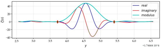
Figure 23. Rogue wave, with very flat waves around: $n=3,206,674$ and $n+1=3,206,675$.

4.4. Model Adherences

4.4.1. The Resemblance with Čebyšëv’s First Function

Čebyšëv’s first function is given by: $\theta \left(x\right)= {\displaystyle \sum }_{p\le x}\ln p;p$ prime.

We know several bounds for this function, for example:

$${\theta }_{p_k}\ge k\left(\ln k+\ln \ln k-1+\frac{\ln \ln k-2.050735}{\ln k}\right) for k\ge {10}^{11};p_k: kth prime number$$

The three-term asymptotic expansion of the Lambert function is as $k$ tends to $+\infty$:

$$W\left(k\right)= \ln k-\ln \ln k+\frac{\ln \ln k}{\ln k}+ \mathcal{O}\left({\left(\frac{\ln \ln k}{\ln k}\right)}^2\right)$$

The connection between the heteroscedasticity of normal distributions and the evolution of the distribution of prime numbers is immediate: ${\theta }_{p_k}\ge kW\left(k\right)+2\ln \ln k$.

We deduce for the primorial $p_m\#$ de $p_m$: $p_m\#= {{\displaystyle \prod }}_{k=1}^m{p}_k; \ln p_m\#={\theta }_{p_m}\ge mW\left(m\right).$

4.4.2. The Rapprochement with the Erdös–Kac Theorem

Probabilistic number theory explicitly uses probabilities to state results on the distribution of properties of natural numbers. $\omega \left(n\right)$ being the number of prime factors distinct from a non-zero natural number $n$, we know the Hardy–Ramanujan theorem [33]: “The normal order of the number $\omega \left(n\right)$ of prime factors distinct from a number $n$ is $\ln \left(\ln n\right)$”. We also know the more precise Erdös–Kac theorem [34]: $\forall 𝜆\in \mathbb{R}: \underset{x\to \infty }{\lim }\frac{1}{x}\left|\right\{n\le x|𝜔(n)\le \ln \ln x+𝜆\sqrt{\ln \ln x}\}|=\frac{1}{\sqrt{2𝜋}}{\int }_{-\infty }^{𝜆}{e}^{-t^2/2}dt$.

This theorem expresses that the number of prime factors distinct from a natural number $n$ for $1<n<N$ tends to a normal distribution with mean $\ln \ln N$ and variance $\ln \ln N$ as $N$ tends to infinity. When running the Eratosthenes sieve to identify prime numbers, which are checked only once, $\omega \left(n\right)$ is the number of scores of each natural number. This number is maximum for primorials ($\mathrm{e}.\mathrm{g}., 7\#=2\times 3\times 5\times 7=210 \Rightarrow \omega \left(210\right)=4$). Thus, we can generate the numbers $n<N={10}^7$ with $\omega \left(n\right)$ prime numbers which follow a more or less bell-shaped histogram: 3 on average, very often (2, 4), less frequently (1, 5), more rarely (6, 7) and only one occurrence for 8: $\forall n\le N={10}^7:1\le \omega \left(n\right)\le 8$. For example:

$$n=2\times 3\times 5=30; n=2^2\times {13}^3\times {29}^2<N ;\omega \left(n\right)=3.$$

$n$ power of a prime number, $n=p_k^m \Rightarrow \omega \left(n\right)=1$:

$$p_{437}=3049; {3049}^2<N;\omega \left(p_{437}\right)=\omega \left(p_{437}^2\right)=1$$

$n$ primorial, $n=p_m\#={{\displaystyle \prod }}_{k=1}^m{p}_k\Rightarrow 𝜔(n)=m$:

$$p_8\#=2 \times 3 \times 5 \times 7\times 11 \times 13 \times 17 \times 19<N; 𝜔(p_8\#)=8$$

To generate all the natural numbers $n<N$, there is an economy principle with the parsimonious use of $\omega \left(n\right)$ prime numbers $\left\{b_n\right\}$ drawn from the elements of the base $B_k≔\{p_1,p_2,\dots ,p_k\};{p_k}^2<N$. As $N$ increases, it is necessary to give more and more flexibility in this number $𝜔$ of prime numbers of the corresponding base. The cardinal of the subset $Card\left(\right\{b_n\left\}\right)$ needs to increase. It seems natural to compare both the evolution of the mean of $𝜔\left(n\right)$ and that of the standard deviation in the $W\left(\ln N\right)\approx \ln \ln N$ of the RV ${\tilde{T}}_n$. The RV needs more flexibility to sweep a larger subset.

4.4.3. The Similarity with the Twin Prime Issue

Twin prime pairs are two prime numbers [35] that differ only by 2. According to the twin primes conjecture, there is an infinity of twin primes $p$ and $p+2$. The occurrence of twin primes can also be related to the Gaussian RV heteroscedasticity. The higher the standard deviation of the normal distribution, the more the prime numbers have the possibility of sweeping a wider range, so much so that two consecutive primes can be joined. Again, to formulate a theory, it might be daring to break away from the natural order of the emergence of prime numbers.

4.5. Pros and Cons of the Model and Numerical Applications

Finally, the model brings theoretical and practical advantages and disadvantages for computational applications:

• This offers an easy way to calculate the numerical value for the seed of the $n^{\mathrm{th}}$ zero: the pivot ${𝓎}_{w5,n}$ is indeed very close to the result.
• The passage through the Fourier transform is clearly improved since the zeta function in the $\tilde{\mathbb{C}}$ space is quasi-periodic, with period 1. It is a fairly regular corrugated sheet and the local Fourier coefficients are then crystallized on a few frequencies, thanks to the resemblance and the correspondence between the Gaussian pdf of a local zero and the local morphology of the zeta function.
• The model has the drawback of being statistical.
• It does not provide answers on questions about the ordering and the numbering of these zeros: it is necessary to deepen the morphological engine of the zeta function and the genesis of the folds of this function.
• The model is valid over a large interval $n< {10}^{20}$, but must be validated for much higher values.

5. Conclusions

The article analyzes numerically the global and local distribution of the non-trivial zeros of Riemann’s zeta function $\zeta \left(s\right)=\zeta \left(x+iy\right)=a+ib= {\displaystyle \sum }_{n=1}^{\infty }{n}^{-s}$ along the CL $ℒ≔\{𝓍=\raisebox{1ex}{$1$}\!\left/ \!\raisebox{-1ex}{$2$}\right.;𝓎>0\}$ of the $\mathbb{C}$ complex plane. The behavior of the $\zeta$ function in the CS (in fact, its analytical extension, since the $\zeta$ function diverges in the CS) is governed in particular by the fractional part $\left\{\tilde{t}\right\}$ of the variable $\tilde{t}=\phi \left(y\right)=y/\left(2\pi \right)\ln \left(y/\left(2\pi e\right)\right)=t \ln \left(t/e\right)=\left[\tilde{t}\right]+\left\{\tilde{t}\right\};t=y/2\pi$.

The $n$ non-trivial zeros ${𝓈}_n$ on $ℒ$ obey the partition of the variable $\tilde{t}$ as follows:

$$\forall n\ge 1:{𝓈}_n=\raisebox{1ex}{$1$}\!\left/ \!\raisebox{-1ex}{$2$}\right.+𝒾{𝓎}_n; \zeta \left({𝓈}_n\right)=0 \Rightarrow \mathfrak{R}\left(\zeta \left({𝓈}_n\right)\right)=\mathfrak{I}\left(\zeta \left({𝓈}_n\right)\right)=0$$

$${\tilde{t}}_n=\phi \left({𝓎}_n\right); \left[{\tilde{t}}_n\right]+\epsilon =n-2 ;\epsilon =-1, 0, +1;{\alpha }_n=\pi /4-2\pi \left\{{\tilde{t}}_n\right\}$$

$${𝜃}_n=-1/(4!{𝓎}_n);{𝜔}_n={𝛼}_n+arg(e^{{i𝜃}_n}+i(1+{i𝜃}_n){𝜃}_n^{3}4!7/5+\cdots )\approx {𝛼}_n+{𝜃}_n$$

$$\underset{𝓈\to {𝓈}_n}{\lim }\frac{\mathfrak{I}(𝜁(𝓈))}{\mathfrak{R}(𝜁(𝓈))}=-\frac{\mathfrak{R}({𝜁}^{\prime }({𝓈}_n))}{\mathfrak{I}({𝜁}^{\prime }({𝓈}_n))}=\tan (\frac{{𝜔}_n}{2})\approx \tan \left(\frac{{𝛼}_n+{𝜃}_n}{2}\right);𝜉({𝓈}_n)=-{\left(\frac{{𝜁}^{\prime }({𝓈}_n)}{|{𝜁}^{\prime }({𝓈}_n)|}\right)}^2$$

This article shows that the zeros are distributed on the CL according to a two-layered hierarchical model $ℳ$.

The first, deterministic layer defines two pivots ${𝓎}_{w1,n}$ and ${𝓎}_{w5,n}$, linked to the $n^{\mathrm{th}}$ zero, close to the cancellation of the imaginary and real parts of the $𝜁$ function, and involves the Lambert function, via an anamorphosis $\phi$: $\phi \left(y\right)=\tilde{t}\iff y=2\pi e^{1+W(\tilde{t}/e)}$.

$$\begin{gathered} \forall n\ge 1: {𝓎}_{w1,n}=2\pi t_{1,n}/W\left(t_{1,n}/e\right); t_{1,n}= n-2+\raisebox{1ex}{$1$}\!\left/ \!\raisebox{-1ex}{$8$}\right.; \zeta \left(\raisebox{1ex}{$1$}\!\left/ \!\raisebox{-1ex}{$2$}\right.+i{𝓎}_{w1,n}\right) \\ ={\epsilon }_n\left(1+i\left(48{𝓎}_{w1,n}+\cdots \right)\right) \end{gathered}$$

$$\begin{gathered} \forall n\ge 1: {𝓎}_{w5,n}=2\pi t_{5,n}/W\left(t_{5,n}/e\right); t_{5,n}= n-2+\raisebox{1ex}{$5$}\!\left/ \!\raisebox{-1ex}{$8$}\right.; \zeta \left(\raisebox{1ex}{$1$}\!\left/ \!\raisebox{-1ex}{$2$}\right.+i{𝓎}_{w5,n}\right) \\ ={ϵ}_n\left(\left(-48{𝓎}_{w5,n}+\cdots \right)+i\right) \end{gathered}$$

$$\left|{\epsilon }_n\right|,\left|{ϵ}_n\right|<\epsilon ; \left(\forall n<{10}^7\Rightarrow \epsilon <1/n\right)$$

$W$ is the main branch of the Lambert function: $W\left(z\right)= w\iff w{e}^w=z ;z\ge -1/e$.

The pivot ${𝓎}_{w5,n}$ turns out to be a good estimate of the ordinate of the $n^{th}$ zero:

$$\forall n\ge 1: {𝓎}_n^{*}={𝓎}_{w5,n}=\frac{2\pi \left(n-2+\raisebox{1ex}{$5$}\!\left/ \!\raisebox{-1ex}{$8$}\right.\right)}{W\left(\frac{n-2+\raisebox{1ex}{$5$}\!\left/ \!\raisebox{-1ex}{$8$}\right.}{e}\right)};\left|{𝓎}_n-{𝓎}_n^{*}\right|<\frac{a}{\ln {𝓎}_n};(a<10 \mathrm{for} n<N={10}^7);$$

An asymptotic estimate for the zero of rank $n$, $z_n=x_n+i{y}_n$ is $\left|{𝓎}_n\right|\approx \frac{2\pi n}{W\left(n/e\right)}\approx \frac{2\pi n}{\ln n}$.

The second, stochastic layer precisely allocates the zeros and involves a sequence of RVs $Y_n={\phi }^{-1}\left({\tilde{T}}_n\right)$. To express the features of the RVs $Y_n~\left({\mu }_n,{\sigma }_n\right)$, it is wiser to work in the anamorphic plane $\tilde{\mathbb{C}}=\phi \left(\mathbb{C}\right)$. In this space $\tilde{\mathbb{C}}$, after a change of variable from $y$ to $\tilde{t}$, the distribution of zeros along the transformed CL follows the realization of a stochastic process of independent Gaussian RVs, regularly spaced: ${\tilde{T}}_n~\mathcal{N}\left({\tilde{\mu }}_n=n,{\tilde{\sigma }}_n{}^2\right); {\tilde{\sigma }}_n=0.1255 W\left(\ln n\right)+0.0886$. The location ${𝓎}_n$ of the nth zero then obeys the probabilistic formula ${𝓎}_n=2\pi {\tilde{t}}_n$ being the realization of the nth RV ${\tilde{T}}_n$, of probability density:

$$f_n\left(\tilde{t}\right)= \frac{1}{{\tilde{\sigma }}_n\sqrt{2\pi } }{e}^{-\raisebox{1ex}{$1$}\!\left/ \!\raisebox{-1ex}{$2$}\right.{\left(\frac{\tilde{t}-n}{{\tilde{\sigma }}_n}\right)}^2}$$

The model $ℳ$ shows that, along the CL, the realizations of adjacent normal distributions overlap, causing irregularities in places, so that the order of neighboring zeros can be swapped. In addition, the distributions ${\tilde{T}}_n$ undergo a slow heteroscedasticity since the standard deviation of the distributions increases in $W\left(\ln n\right)$.

The model $ℳ$ makes it possible to calculate the respective zeros of the real and imaginary parts:

$$\begin{gathered} \forall n: {𝓈}_{5,n}=\raisebox{1ex}{$1$}\!\left/ \!\raisebox{-1ex}{$2$}\right.+𝒾\left({𝓎}_{w5,n}+{\left(4!{𝓎}_{w5,n}\ln \left(\frac{{𝓎}_{w5,n}}{2\pi }\right)-\frac{1}{{𝓎}_{w5,n}}+\cdots \right)}^{-1}\right); \\ \xi \left({𝓈}_{5,n}\right)=-1;\zeta \left({𝓈}_{5,n}\right)=i{𝒷}_n\in i\mathbb{R} \end{gathered}$$

$$\begin{gathered} \forall n:{𝓈}_{1,n}=\raisebox{1ex}{$1$}\!\left/ \!\raisebox{-1ex}{$2$}\right.+𝒾\left({𝓎}_{w1,n}+{\left(4!{𝓎}_{w1,n}\ln \left(\frac{{𝓎}_{w1,n}}{2\pi }\right)-\frac{1}{{𝓎}_{w1,n}}+\cdots \right)}^{-1}\right); \\ \xi \left({𝓈}_{1,n}\right)=+1;\zeta \left({𝓈}_{1,n}\right)={𝒶}_n\in \mathbb{R} \end{gathered}$$

The model $ℳ$ reveals the direct relation between the two $\zeta$ components on the whole CL $ℒ$:

$$\forall 𝓈=\raisebox{1ex}{$1$}\!\left/ \!\raisebox{-1ex}{$2$}\right.+𝒾𝓎 \in ℒ : \frac{\mathfrak{I}\left(\zeta \left(𝓈\right)\right)}{\mathfrak{R}\left(\zeta \left(𝓈\right)\right)}=\tan \left(\frac{\omega }{2}\right);\omega =\alpha +\theta +\cdots ; \alpha =\frac{\pi }{4}-2\pi \left\{\phi \left(𝓎\right)\right\}; \theta =-\frac{1}{4!𝓎}$$

$$\xi \left(𝓈\right)=e^{i\omega }\approx e^{i\alpha }\left(e^{i\theta }+\frac{168{\theta }^{3}i}{5}\left(1+i\theta \right)\right)\approx e^{i\left(\alpha +\theta \right)}$$

This two-layer distribution model helps to deduce the known results or to specify laws already studied in the literature:

• The sequence number $n$ of zero $𝓎$ is: $n=\left[𝓎/\left(2\pi \right)\ln \left(𝓎/\left(2\pi e\right)\right)-\raisebox{1ex}{$1$}\!\left/ \!\raisebox{-1ex}{$8$}\right.\right]+2$, the error is $-1, 0, +1$, according to the probabilities $0.065, 0.87, 0.0065$, when $n<N \cong {10}^7$.
• The law of the number of zeros $\le 𝓎$: $N\left(𝓎\right)=t\ln \left(t/e\right)-\raisebox{1ex}{$1$}\!\left/ \!\raisebox{-1ex}{$8$}\right.+1+\omega /2\pi ;\zeta \left(𝓈\right)=a+ib;a>0$. The last term depends on $sign\left(a\right), sign\left(b\right)$, i.e., on which quadrant is $\zeta \left(𝓈\right)$.
• The law of the differences of the ordinates of consecutive zeros is a $\Delta Y$ law, associated with the normal law $\Delta \tilde{T}~\mathcal{N}\left(1,{\tilde{\sigma }}_n\right)$. The mean $\Delta {𝓎}_n$ is valued:

  $$\Delta {𝓎}_n= {𝓎}_{n+1}-{𝓎}_n= \frac{2\pi }{W\left(\frac{n-2+\raisebox{1ex}{$5$}\!\left/ \!\raisebox{-1ex}{$8$}\right.}{e}\right)}= \frac{2\pi }{\ln \left(\frac{{𝓎}_n}{2\pi e}\right)}; \Delta t_n\times \ln \left(t_n/e\right)=1$$
  We use here the natural order of zeros, that is to say that we admit, in this formula, the dependence between two consecutive RVs (${𝓎}_{n+1}>{𝓎}_n$).
• The common law of the maximum of the absolute value of $\zeta \left(𝓈\right)$ in its real and imaginary components, and in absolute value:

  $$M_0\left(𝓎\right)=\underset{u<y}{\max }\left|\zeta \left(\raisebox{1ex}{$1$}\!\left/ \!\raisebox{-1ex}{$2$}\right.+iu\right)\right|=\underset{u<y}{\max }\left|\mathfrak{R}\left(e^{i\pi /4}\zeta \left(\raisebox{1ex}{$1$}\!\left/ \!\raisebox{-1ex}{$2$}\right.+iu\right)\right)\right|=\underset{u<y}{\max }\left|\mathfrak{I}\left(e^{i\pi /4}\zeta \left(\raisebox{1ex}{$1$}\!\left/ \!\raisebox{-1ex}{$2$}\right.+iu\right)\right)\right|$$

  $$M_0\left(𝓎\right)\approx 2.865 {𝓎}^{0.195}\approx 0.921\left({𝓎}^{0.128}{\left(\ln 𝓎 \right)}^{0.786}\right)$$
  The rotation of $\pi /4$ restores the balance between the two components.
• The moments $M_k\left(𝓎\right)=\frac{1}{𝓎}{{\displaystyle \int }}_0^{𝓎}{\left|\zeta \left(\raisebox{1ex}{$1$}\!\left/ \!\raisebox{-1ex}{$2$}\right.+iu\right)\right|}^{k}du$:

  $$M_1\left(𝓎\right)\approx -0.00661\ln 𝓎 + 0.694\ln \ln 𝓎 +0.357; M_3\left(𝓎\right)\approx \frac{0.86375}{2{\pi }^2}{\left(\ln 𝓎\right)}^3+ 16.53$$

  $$M_2\left(𝓎\right)\approx \ln 𝓎 +2\gamma -1-\ln 2\pi =\ln 𝓎 -1.68344$$

  $$M_4\left(𝓎\right)\approx \frac{1}{2{\pi }^2}{\left(\ln 𝓎\right)}^4+0.123 {\left(\ln 𝓎\right)}^3 -0.748{\left(\ln 𝓎\right)}^2+1.402\ln 𝓎-0.816$$
• The moments $M_{2k}\left(𝓎\right)={{\displaystyle \int }}_0^{𝓎}{\left|\zeta \left(\raisebox{1ex}{$1$}\!\left/ \!\raisebox{-1ex}{$2$}\right.+iu\right)\right|}^{2k}du={𝓎}^{\frac{k+2}{4}}{\left(\ln 𝓎\right)}^k \mathcal{O}\left({\left(\ln 𝓎\right)}^{ϵ\left(k\right)}\right)$:
  $$ϵ\left(3\right)=1.072;ϵ\left(4\right)=0.624;ϵ\left(5\right)=0.418;ϵ\left(6\right)=0.396$$

The model also makes it possible to spot a family of local profiles of the $\zeta$ function on the CL, around the RVs, according to the realization of the neighboring Gaussian RV. This family can be extended to the entire CS, thanks to the homothety of the morphologies of the $\zeta$ function in the CS. If the value ${𝓎}_n$ deviates a little from the mean ${\mu }_n$ of the RV $Y_n$, the $\zeta$ function profile is regular around this neighborhood: the real and imaginary waves are almost stationary with sinusoids of similar amplitudes. On the other hand, if the value ${𝓎}_n$ is significantly different from the mean of the RV $Y_n$, a “rogue wave” emerges, in the vicinity of the value $𝓎={\mu }_n$, worthy of the Roaring Forties, which contributes to the development of local maxima of $\zeta \left(s\right)$ on the CL and in the CS (for $x=0$). This very high wave is then accompanied by waves of tiny amplitudes, in dead calm, which cause the emergence of close consecutive zeros.

Finally, the hierarchical model allows us to explain the absence of multiple roots, by dissecting Hadamard’s product formula, with two close zeros.

The numerical study of the Gaussian RV ${\tilde{T}}_n$. must be continued, in particular the slow evolution of its heteroscedasticity, which must be validated for high values of $n;n>N\approx {10}^{100}$. Indeed, the very slow growth of the standard deviation would be a major property of the second layer of the model, which would reflect the local disorder of non-trivial zeros, notably in their distributions for very low probability densities ($<{10}^{-10}$) of ${\tilde{T}}_n$, analyzable by the theory of extremes, and in relation to the distribution of prime numbers for very high values.

The $𝜁$ function contains secrets that we can unravel through new analysis grids. The digital way offers to openly illustrate drafts of research. In this article, the Lambert function, by its elongation, reveals the uniform description of folds of the Zeta function along the transformed imaginary axis and the normal distribution locally distributes the zeros around regularly spaced pivots. Lambert’s unfolding standardizes the global aspect of the Zeta function in equivalent paradigms of length 1, but the stress relief of Gauss’s law, along $n$, expresses a progressive degree of freedom of the local position of the zeros, thanks to the increasing standard deviation in $\ln \left(\ln n\right)$, most certainly, in relation with the Erdös–Kac theorem and with the maximum elasticity (perceptible on twin prime numbers) of the distribution of prime numbers for very high values of $n$.

References

- Riemann, B. Über die Anzahl der Primzahlen unter Einer Gegebenen Größe. Ges. Math. Werke und Wissenschaftlicher Nachlaß 1859, 2, 145–155. [Google Scholar]
- Lambert, J.H. Observationes Variae in Mathesin Puram. Acta Helv. Phys. Math. Anat. Bot. Med. 1758, 3, 128–168. [Google Scholar]
- Hadamard, J. Sur les zéros de la fonction de Riemann. Comptes Rendus de l’Académie Sci. Paris 1896, 122, 1470–1473. [Google Scholar]
- De la Vallée Poussin, C.-J. Sur la fonction de Riemann et le nombre des nombres premiers inférieurs à une limite donnée. Sci. Lett. Beaux-Arts Belg. 1899, 49, 74. [Google Scholar]
- Gram, J.-P. Note sur les zéros de la fonction de Riemann. Acta Math. 1903, 27, 289–304. [Google Scholar] [CrossRef]
- Landau, E. Über die Nullstellen der Zeta-funktion. Math. Ann. 1912, 71, 548–564. [Google Scholar] [CrossRef]
- Hardy, G.H. Sur les zéros de la fonction de Riemann. C. R. Acad. Sci. Paris 1914, 158, 1012–1014. [Google Scholar]
- Littlewood, J.E. On the zeros of the Riemann zeta-function. Proc. Camb. Philos. Soc. 1924, 22, 295–318. [Google Scholar] [CrossRef]
- Levinson, N. More than one third of zeros of Riemann’s zeta-function are on σ = ½. Adv. Math. 1974, 13, 383–436. [Google Scholar]
- Conrey, J.B. More than two fifths of the zeros of the Riemann zeta function are on the critical line. J. Reine Angew. Math. 1989, 399, 1–26. [Google Scholar]
- Hardy, G.H.; Littlewood, J.E. The zeros of Riemann’s zeta function on the critical line. Math. Z. 1921, 10, 283–317. [Google Scholar] [CrossRef]
- Atkinson, F.V. The mean value of the zeta-function on the critical line. Proc. Lond. Math. Soc. 1941, 47, 174–200. [Google Scholar]
- Ingham, A.E. On the estimation of N(σ,T). Quart. J. Math. 1940, 11, 291–292. [Google Scholar] [CrossRef]
- Odlyzko, A. Tables of Zeros of the Riemann Zeta Function. 2002. Available online: http://www.dtc.umn.edu/~odlyzko/zeta_tables/index.html (accessed on 11 December 2020).
- Gourdon, X. The 1013 First Zeros of the Riemann Zeta Function, and Zeros Computation at Very Large Height. 2004. Available online: http://numbers.computation.free.fr/Constants/Miscellaneous/zetazeros1e13-1e24.pdf (accessed on 11 December 2020).
- Titchmarsh, E.C. The theory of the Riemann Zeta-Function, 1st ed.; Oxford Univ. Press: Oxford, UK, 1951; p. 346. [Google Scholar]
- Ivić, A. The Riemann Zeta-Function. The Theory of the Riemann Zeta-Function with Applications; John Wiley & Sons: New York, NY, USA, 1985; 517p. [Google Scholar]
- Selberg, A. On the zeros of Riemann’s zeta-function. Skr. Norske Vid. Akad. Oslo I 1942, 10, 1–59. [Google Scholar]
- Backlund, R.J. Sur les zéros de la fonction de Riemann. C. R. Acad. Sci. Paris 1914, 158, 1979–1981. [Google Scholar]
- Karatsuba, A.A. On the zeros of the Riemann zeta-function on short intervals of the critical line. Sov. Math. Dokl. 1983, 28, 533–535. [Google Scholar]
- Feng, S.; Wu, X. On gaps between zeros of the Riemann zeta-function. J. Number Theory 2012, 132, 1385–1397. [Google Scholar] [CrossRef][Green Version]
- Montgomery, H.L. The pair correlation of zeros of the zeta function. In Analytic Number Theory (Proc. Symp. Pure Math., Vol. 24); American Mathematical Society: Providence, RI, USA, 1973; pp. 181–193. [Google Scholar]
- Conrey, J.B.; Ghosh, A. A conjecture for the sixth power moment of the Riemann zeta function. In Proceedings of the Amalfi Conference on Analytic Number Theory, Maiori, Italy, 25–29 September 1989; pp. 35–59. [Google Scholar]
- Conrey, J.B.; Gonek, S.M. High moments of the Riemann zeta-function. Duke Math. J. 2001, 107, 577–604. [Google Scholar] [CrossRef]
- Laplace, P.S. Théorie Analytique des Probabilités; Œuvre Tome VII; Courcier: Paris, France, 1820; ISBN 978-2-87647-161-0. [Google Scholar]
- Čebyšëv, P.L. Mémoire sur les nombres premiers. J. Math. Pures Appl. 1852, 17, 366–390. [Google Scholar]
- Lévy, P. Théorie de L’addition des Variables Aléatoires; Gauthier-Villars: Paris, France, 1937; ISBN 978-2-87647-207-5. [Google Scholar]
- Poisson, S.D. Recherches sur la Probabilité des Jugements en Matière Criminelle et en Matière Civile, Précédée des Règles Générales du Calcul des Probabilités; Bachelier: Paris, France, 1837. [Google Scholar]
- Fisher, R.A.; Tippett, L.H.C. Limiting forms of the frequency distribution of the largest or smallest member of a sample. Proc. Camb. Philos. Soc. 1928, 24, 180–190. [Google Scholar] [CrossRef]
- Gumbel, E.J. Statistics of Extremes; Columbia University Press: New York, NY, USA, 1958. [Google Scholar]
- Fréchet, M. Sur la loi de probabilité de l’écart maximum. Ann. Soc. Polonaise Math. 1927, 6, 92–116. [Google Scholar]
- Weibull, W. A statistical distribution of wide applicability. J. Appl. Mech. 1951, 18, 293–297. [Google Scholar]
- Hardy, G.H.; Ramanujan, S. The normal number of prime factors of a number n. Quart. J. Math. 1917, 48, 76–92. [Google Scholar]
- Erdős, P.; Kac, M. The Gaussian law of errors in the theory of additive functions. Proc. Natl. Acad. Sci. USA 1939, 25, 206–207. [Google Scholar] [CrossRef] [PubMed]
- Korevaar, J. Prime pairs and the zeta function. J. Approx. Theory 2009, 158, 69–96. [Google Scholar] [CrossRef][Green Version]
Publisher’s Note: MDPI stays neutral with regard to jurisdictional claims in published maps and institutional affiliations. |
© 2021 by the author. Licensee MDPI, Basel, Switzerland. This article is an open access article distributed under the terms and conditions of the Creative Commons Attribution (CC BY) license (http://creativecommons.org/licenses/by/4.0/).