Article

Fusion of Angle Measurements from Hull Mounted and Towed Array Sensors

by
Kausar Jahan
* and
Koteswara Rao Sanagapallea
Department of Electronics and Communication Engineering, Koneru Lakshmaiah Education Foundation, Vaddeswaram, Guntur 522502, Andhra Pradesh, India
*
Author to whom correspondence should be addressed.
Information 2020, 11(9), 432; https://doi.org/10.3390/info11090432
Submission received: 7 July 2020 / Revised: 31 August 2020 / Accepted: 5 September 2020 / Published: 9 September 2020
(This article belongs to the Special Issue Data Modeling and Predictive Analytics)

Abstract

:
Two sensor arrays, hull-mounted array, and towed array sensors are considered for bearings-only tracking. An algorithm is designed to combine the information obtained as bearing (angle) measurements from both sensor arrays to give a better solution. Using data from two different sensor arrays reduces the problem of observability and the observer need not follow the S-maneuver to attain observability of the process. The performance of the fusion algorithm is comparable to that of theoretical Cramer–Rao lower bound and with that of the algorithm when bearing measurements from a single sensor array are considered. Different filters are used for analyzing both algorithms. Monte Carlo runs need to be done to evaluate the performance of algorithms more accurately. Also, the performance of the fusion algorithm is evaluated in terms of solution convergence time.

1. Introduction

The demand for fast and accurate tracking of the targets is increasing day by day. Under water, noise corrupted angle measurements are available from noise radiated from the target and processed from a single observer platform operating in passive mode [1]. Passive target tracking is more popular as it helps the tracker from being tracked. In the ocean environment, target motion analysis is generally performed in a two-dimensional plane using angles-only measurements. The angles generated by the sensors are well known as bearing angles. The observer with the single sensor array, say hull-mounted array (HMA), in a passive mode, determines parameters of target motion like its range, course, bearing angle, speed, etc. As the range of the target is not available and bearing being nonlinearly related to target motion parameters, nonlinearity in the process is high [2]. In addition to this, measurements from a single sensor array are only considered to be available, which makes the process unobservable and the observer must perform a proper maneuver to make the process observable [3,4,5].
The ocean environment is unstable all the time and this makes the bearing measurements from a single sensor array unreliable in obtaining all the required information about the target. Moreover, an increase in system complexity increases the need for more input from different sensor arrays to obtain complete information on the system. According to the application and need, a system with multiple sensors can choose different sensors with the required characteristics and based on the environmental conditions for obtaining the target information. Information from these sensors is then consistently combined coherently to obtain the parameters like range, course, velocity, and acceleration of the target during its movement. This is known as data fusion problem. As the bearing measurements are taken from two sensors, in this work, the maneuver of the observer to obtain the observability of the target is reduced in most of the scenarios.
Angles-only tracking, commonly known as bearings-only tracking, used classical filters like maximum likelihood estimator, pseudo linear estimator, etc. in the early 19th century [1,6] and these were batch processing filters. In real-time scenarios, these batch processing estimators need a lot of time for obtaining the estimated results. This led to the evolution of recursive estimators like least square estimator, Kalman filter (KF), etc. KF being a linear filter was not suitable for nonlinear bearings-only tracking [3]. The nonlinearity in the process leads to the evolution of extended KF (EKF), unscented KF (UKF), particle filter (PF), etc. to deal with the nonlinearities in the process and measurements [7]. EKF reduces the nonlinearities by linearizing the measurement equation using Taylor series expansion and updates the state and covariance matrices and calculates the filter gain. The filter is mostly dependent on the initializations and due to the linearization process; information is lost making the solution unreliable. In UKF, the probability density function of the state vector is propagated through a set of carefully chosen sample points, called sigma points, using unscented transform [8,9]. This helps in possession of posterior mean and covariance up to second order for any type of nonlinearity. Hence, unlike EKF, UKF can provide improved stability, accuracy, and better convergence in solution [10,11,12].
Y. Bar-Shalom, in [13], gave a deep insight regarding data association and data fusion of multiple sensors in multiple target environment using radar measurements. Several filtering algorithms were utilized including EKF, UKF, and PF. Data fusion for underwater surveillance was presented in [14,15,16], in which the technique was evaluated only using MGBEKF and UKF algorithms. In [17], the author used a data fusion technique to evaluate the performance of the fusion technique for two and more than two sensors of data fusion. It is an extensive work for the work presented by Bar-Shalom on data fusion. In [18], the authors applied a data fusion technique using a PF for estimation of robot motions. In [19], the authors analyzed the fusion technique for batch processing using the maximum likelihood estimator and analyzed the same with recursive processing with an unscented Gauss–Helmert Kalman filter. The observability of the system is further discussed in the paper. In [18], a data fusion algorithm was used along with a data association algorithm to detect multiple targets. It deals with the hardware complexity in target detection. In [19], data fusion was used to detect the target in a properly designed underwater network. In [20], authors used interacting multiple model techniques combined with EKF and UKF for tracking the single as well as multiple targets and compared two different data fusion techniques that involve fusion using nearest neighborhood calculation and fusion using probabilistic data association. The data fusion techniques in literature are extended to robotics, in air surveillance, and underwater surveillance applications. However, there is a necessity to explore the fusion techniques in detail for underwater surveillance applications.
The filters considered for evaluation of fusion algorithm are further compared with theoretical Cramer–Rao lower bound (CRLB). The mathematical modelling of CRLB for tracking algorithms using a single sensor array is in [9,21] and that for tracking algorithms using two sensor arrays is represented in Section 2.6.
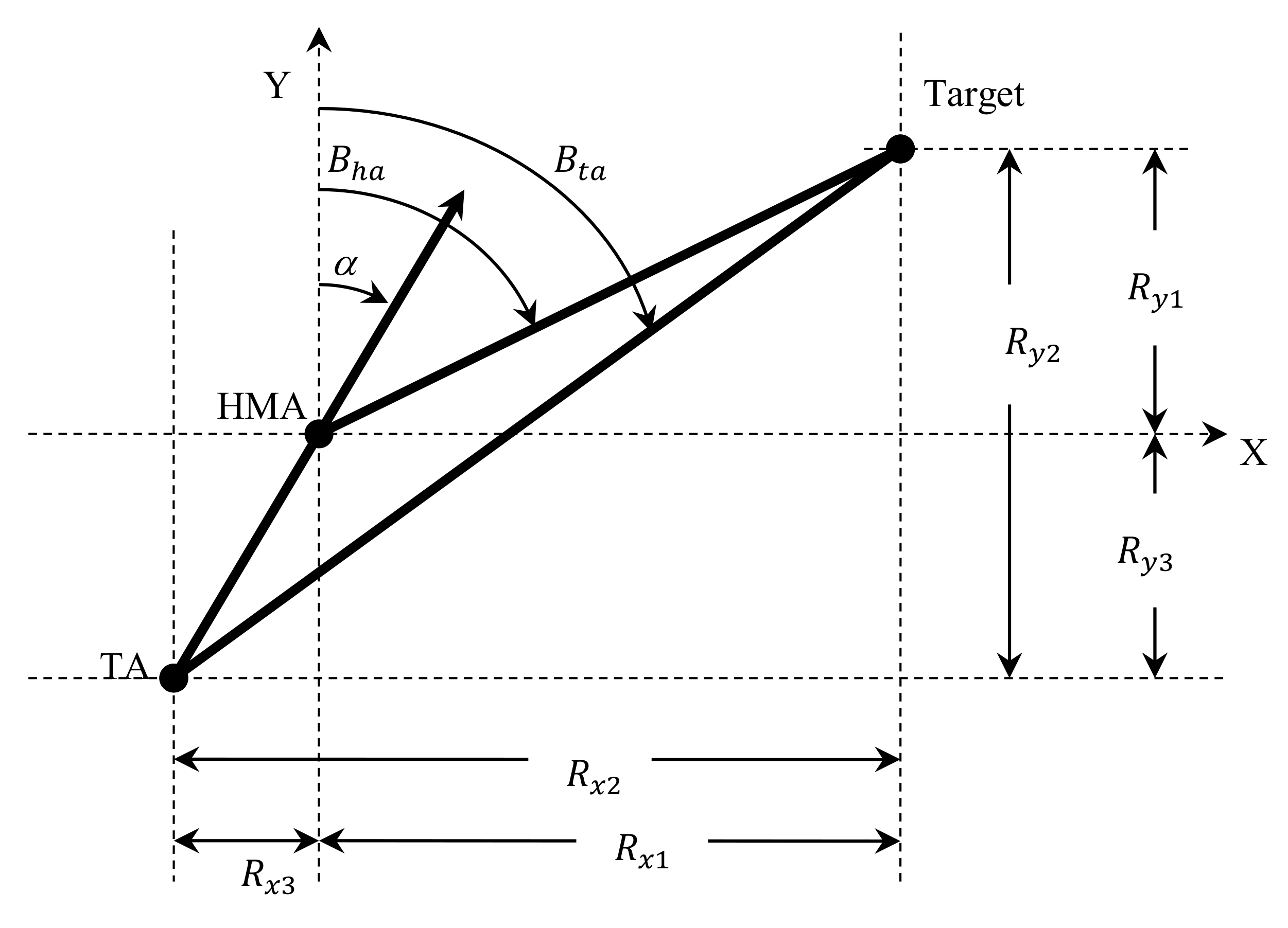
In this paper, a single target following the constant velocity model is considered for simplicity. The fusion of measurement information from two sensor arrays, HMA and towed array (TA) is considered without maneuver. TA is towed behind the observer at a certain distance away from the observer. This helps in the reduction of self-noise from the observer and allows it to operate at very low frequencies. Hence, the TA will be capable of even tracking the target at great distances. The algorithm is evaluated for several scenarios in Monte Carlo simulations.
In this paper, the performance of BOT with a single sensor (HMA) and two sensors (HMA and TA) using different filters is evaluated. The mathematical modelling of all the algorithms is described in Section 2. The results obtained from the simulation of the algorithms and discussion on the results is given in Section 3. This paper is concluded in Section 4.

2. Mathematical Modeling

2.1. Tracking Using a Single Sensor Array

Tracking using a single sensor array (SST) measurement considers the bearing measurements from HMA only. The observer is assumed to be following constant speed with S—the maneuver in the course and the target follows persistence speed and course [20]. At time instant, say ‘ τ ’, state vector of the observer [9,10] is given as Equation (1).
S o τ = v x o τ v y o τ r x o τ r y o τ T .
Here v x o τ , v y o τ , r x o τ , r y o τ are the respective speeds and ranges of the observer in x and y coordinates. With the known speed and course of the observer, change in the observer’s x and y position is obtained as Equations (2) and (3).
d r x o τ = v x o τ sin o c r τ ,
d r y o τ = v y o τ cos o c r τ .
Here d r x o τ is the change in x coordinate and d r y o τ is the change in y coordinates of observer. o c r is the observer course with τ being the time of a second. The state vector of the target is given as Equation (4).
S t τ = v x t τ v y t τ r x t τ r y t τ T .
Here v x t τ , v y t τ , r x t τ , r y t τ represent target’s speed and range values in x and y coordinates respectively. Target position, when its course and speed are known, changes according to the following Equations (5) and (6).
d r x t τ = v x t τ sin t c r τ ,
d r y t τ = v y t τ cos t c r τ .
Here d r x t τ ,   d r y t τ are the progress in x and y coordinates of the target. t c r is the target course and τ is the time of one second. The target’s state vector relative to the observer [9,12,13] is as in Equation (7).
S s τ = v x τ v y τ r x τ r y τ T .
Here v x τ , v y τ , r x τ , r y τ are relative values of respective speed and range in x and y coordinates. The state vector of the target relative to the observer for the proceeding time, concerning the relative target state vector at present is given as Equation (8).
S s τ + 1 = A τ S s τ + b τ + 1 + ω C τ .
Here A τ is the system dynamics matrix given as Equation (9) and b τ is the deterministic matrix given as in Equation (10).
A τ = 1 0 0 0 0 1 0 0 τ 0 1 0 0 τ 0 1 ,
b τ + 1 = 0         0       r x o τ + 1 r x o τ         r y o τ + 1 r y o τ T .
Here C τ is the system noise and its gain matrix, ω is taken as in Equation (11).
ω = τ 0 0 τ τ 2 / 2 0 0 τ 2 / 2
Let Q τ be the covariance of system noise. Then it is given as in Equations (12) and (13).
Q τ = E ω C τ ω C τ T ,
Q τ = σ 2 τ 2 0 τ 3 / 2 0 0 τ 2 0 τ 3 / 2 τ 3 / 2 0 τ 4 / 4 0 0 τ 3 / 2 0 τ 4 / 4 .
Here σ 2 is taken as the variance of system noise multiplied with some constant value as given in (13). The measurement equation for SST has bearing angles from single sensor array (HMA) and the bearing angle β τ is given as in Equation (14).
β τ = tan 1 r x τ / r y τ .
Measured bearing, β m τ , degraded with noise is obtained and is mathematically expressed as in Equation (15).
β m τ = β τ + η τ .
Here η τ is the noise in the measurement. Here zero-mean additive process noise and measurement noise are considered. The system measurement equation is given as in Equation (16).
Z τ = H τ S s τ + γ τ .
Here H τ matrix gives the relation between measurement and state of the system and the measurement noise matrix is represented by γ τ .

2.2. Tracking Using Two Sensor Arrays

For target tracking using two sensor arrays (TST), the bearing measurements from HMA and TA are considered. Consider the true bearing angles from HMA and TA be β h a 1 ,     β h a 2 ,     β h a 3 ,     ,     β h a τ and β t a 1 ,   β t a 2 ,   β t a 3 ,   ,   β t a τ respectively where τ represents the time. Measurement vector, β m τ can be written as in Equation (17).
β m τ = β h a m τ β t a m τ T ,
τ represents the time for which the measurement vector is considered. The relative target state vector, that is taken concerning observer be S S τ , is given as in Equation (18).
S S τ = v ˙ x τ v ˙ y τ v x τ v y τ r x τ r y τ T .
Here, v ˙ x τ , v ˙ y τ , v x τ , v y τ , r x τ , and r y τ are corresponding acceleration, corresponding speed and corresponding range components of the target concerning observer. The dynamic equation of the target state is given as in Equations (19) and (20).
S S τ + 1 = A τ + 1 S S τ + b τ + 1 + ω C τ ,
b τ + 1 = 0         0         0         0         r x o τ + 1 r x o τ         r y o τ + 1 r y o τ T .
Here A is the transition matrix and is given as in Equation (21) and ω is taken as in Equation (22).
A τ + 1 = 1 0 0 0 0 0 0 1 0 0 0 0 τ 0 1 0 0 0 0 τ 0 1 0 0 τ 2 / 2 0 τ 0 1 0 0 τ 2 / 2 0 τ 0 1 ,
ω = 1 0 τ 0 τ 2 / 2 0 0 1 0 τ 0 τ 2 / 2 T .
The plant noise ω τ is assumed to follow Gaussian distribution. It is given by Equation (23).
C τ = C x ¨ C y ¨ T .
The plant noise covariance matrix is given Equations (24) and (25).
Q τ = E ω C τ C T τ ω T ,
Q τ = 1 0 τ 0 τ 2 / 2 0 0 1 0 τ 0 τ 2 / 2 τ 0 τ 2 0 τ 3 / 2 0 0 τ 0 τ 2 0 τ 3 / 2 τ 2 / 2 0 τ 3 / 2 0 τ 4 / 4 0 0 τ 2 / 2 0 τ 3 / 2 0 τ 4 / 4 × E C τ C T τ .
Initially, HMA is assumed to be at origin and TA is L meters apart from HMA and towed behind the ship. Figure 1 represents the initial positions of HMA, TA, and target. Let R x 1 ,   R y 1 and R x 2 ,   R y 2 be x and y coordinates of target range corresponding to HMA and TA. The observer is assumed to be moving with a course of α concerning the Y-axis. B t a and B h a are the true bearing angles concerning TA and HMA. R x 3 ,   R y 3 is the location of TA concerning HMA and is assumed to be 500m apart from HMA.
From Figure 1, R x 3 and R y 3 are given by Equations (26) and (27).
R x 3 = L sin α + 180 ,
R y 3 = L cos α + 180 .
From Figure 1, the relation between range coordinates can be written as in Equations (28) and (29).
R x 2 = R x 1 + R x 3 ,
R y 2 = R y 1 + R y 3 .
The HMA bearing, β h a m is modelled as in Equation (30).
β h a m τ = tan 1 R x 1 τ R y 1 τ + γ h a β τ ,
where γ h a β τ is an error in the HMA measurement and is assumed to follow zero-mean Gaussian distribution with variance σ h a β 2 τ . The measurement and plant noises are assumed to be uncorrelated to each other. Measured bearing from TA, β t a m τ is given as in Equation (31).
β t a m τ = tan 1 R x 2 τ / R y 2 τ + γ t a β τ .
Here, error in TA measurement is represented as γ t a β τ and is assumed to follow Gaussian distribution with zero mean and having variance of σ t a β 2 τ .
The covariance matrix of the measurements, τ , at time τ is taken as in Equation (32).
τ = σ h a β 2 τ 0 0 σ t a β 2 τ .

2.3. Algorithm of Extended Kalman Filter for TST

The main idea of EKF is to linearize the existing non-linearities in measurement as well as state equations and then perform Kalman filtering. The nonlinearity in this application is considered only in the measurement Equation (16) [20]. Therefore, a partial derivation is applied to the measurement model matrix for linearization and is linearized measurement model matrix for HMA, H h a is obtained as follows in Equation (33).
H h a τ + 1 = 0         0         0         0         R ^ y 1 τ + 1 , τ R ^ 1 2 τ + 1 , τ         R ^ x 1 τ + 1 , τ R ^ 1 2 τ + 1 , τ .
Here R 1 2 = R x 1 2 + R y 1 2
The true parameters of the target are not known in real-time scenarios, so the estimated values, R ^ x 1 , and R ^ y 1 are used in Equation (33). Measurement matrix of TA, H t a is given by Equation (34).
H t a τ + 1 = 0         0         0         0         R ^ y 2 τ + 1 , τ R ^ 2 2 τ + 1 , τ         R ^ x 2 τ + 1 , τ R ^ 2 2 τ + 1 , τ .
Here R 2 2 = R x 2 2 + R y 2 2 .
Measurement fused matrix, H is given by Equation (35).
H τ + 1 = H h a τ + 1 H t a τ + 1 T .
The priori state vector estimation is calculated as follows in Equation (36).
S s τ + 1 | τ = A τ S s τ | τ .
The estimated priori state covariance matrix estimation [2] is done as follows in Equation (37).
P τ + 1 | τ = A τ P τ | τ A τ T + Q τ .
The gain [2] is calculated for EKF as in Equation (38).
G τ = P τ + 1 | τ H T τ H τ P τ + 1 | τ H T τ + τ 1 .
The posteriori state and its covariance matrices, based on the measurements, are updated respectively as follows in Equations (39) and (40).
S s τ + 1 | τ + 1 = S s τ + 1 | τ + G τ Z τ ,
P τ + 1 | τ + 1 = I G τ H τ P τ + 1 | τ I G τ H τ T + G τ τ G τ T .

2.4. Algorithm of Modified Gain Bearings-Only Extended Kalman Filter for TST

The modified gain function, g h a [12] is given by Equation (41).
g h a = 0         0         0         0         cos β h a m R ^ x 1 sin β h a m + R ^ y 1 cos β h a m         sin β h a m R ^ x 1 sin β h a m + R ^ y 1 cos β h a m ,
and TA’s modified gain function, g t a can be written as in Equation (42).
g t a = 0         0         0         0         cos β t a m R ^ x 2 sin β t a m + R ^ y 2 cos β t a m         sin β t a m R ^ x 2 sin β t a m + R ^ y 2 cos β t a m .
Finally, g is written as in Equation (43).
g = g h a g t a T .
The predicted covariance matrix is calculated as in Equation (44).
P τ + 1 = A τ + 1 P τ A T τ + 1 + ω C τ + 1 ω T .
The Kalman gain is calculated as in Equation (45).
G τ + 1 = P τ + 1 H T τ + 1 τ + H τ + 1 P τ + 1 H T τ + 1 1 .
The updated state matrix is calculated as in Equation (46).
S s τ + 1 = S s τ + 1 + G τ + 1 Z τ + 1 Z τ + 1 , S s τ + 1 .
Here Z τ + 1 ,   S s τ + 1 is the bearing measurement obtained from predicted estimate at time index τ + 1 . The updated covariance matrix is given in Equation (47).
P τ + 1 = I G τ + 1 g β m τ + 1 , S s τ + 1 P τ + 1 I G τ + 1 g β m τ + 1 , S s τ + 1 T + τ G τ + 1 G T τ + 1 .

2.5. Particle Filter Combined with Other Filters

PF [12] is an advanced nonlinear filter, suitable for systems that are nonlinear and applicable in the non-Gaussian environment. In PF, estimation is done by considering the probability density function (PDF) of the state vector. Initially, a set of N random state vectors are generated based on the initial PDF of the state, p S S 0 | 0 , which is assumed to be a known value [21]. These randomly generated state vectors are called particles and are represented as S S n , τ | τ n = 1 , 2 , , N . These particles are propagated to the next time using (48).
S S n , τ + 1 | τ = f S S n , τ | τ , C τ + 1 ,   n = 1 , 2 , ,   N
Here, C is the plant noise that is generated randomly based on the PDF of the particle. Once the measurements are obtained, the conditional relative likelihood of each particle, p Z τ ,   S S n , τ + 1 | τ , is computed. For an m-dimensional measurement equation, a relative likelihood O τ can be computed as follows in Equation (49) [12].
O τ = P Z τ = Z , S S n , τ = S S n , τ + 1 | τ = P γ τ = Z H S S n , τ + 1 | τ ~ 1 / 2 π m / 2 σ B 2 m / 2 × e x p Z H S S n , τ + 1 | τ T Z H S S n , τ + 1 | τ 2 σ B 2
~ ’ symbol in (47) represents the proportionality relation rather than the equality relation between the probability and expression on the right side. Now the relative likelihoods obtained in (46) are normalized as follows in Equation (50).
O τ = O τ / i = 1 N O i
Now, the particles using the computed likelihoods are re-sampled. This means a new set of particles are randomly generated based on the relative likelihoods O τ . As the number of particles increases to infinity, the accuracy in estimation increases and thereby complexity of computation. At any point in time, these sets of particles can approximate the PDF of the state accurately [21]. The advanced microprocessors, available these days can easily manage the complexity in computation regarding PF.
It is a known fact that PF has the disadvantage of high computational complexity, but this disadvantage can be reduced by the utilization of fast computing processors with high storage memory (which are available now a days). PF also has the disadvantage of sample degeneracy and sample impoverishment. This is reduced by several resampling techniques available in literature [9,22]. However, these techniques are not suitable for all types of applications. Based on application, proper sampling technique must be selected.
One approach that has been proposed for improving particle filtering is to combine it with another filter such as the EKF, UKF, or MGBEKF [12]. Here, each posterior particle will be updated using the posterior updating equations of EKF, UKF, or MGBEKF algorithms and then re-sampling (if required) is performed. This is like working with an N number of Kalman filters (one for each particle), that is initialized with randomly generated state vectors and then re-sampling them (if required) after updating them with each measurement obtained. In this research work, PF combined with the EKF algorithm is explained for fused measurement data in the form of a flowchart in Figure 2. Similarly, PF is combined with MGBEKF. In this paper, the particle filter is combined with the EKF, MGBEKF and the algorithms are named as particle filter coupled with extended Kalman filter (PFEKF) and particle filter coupled with modified gain bearings-only extended Kalman filter (PFMGBEKF). S S n , τ + 1 | τ is updated to S S n , τ + 1 | τ + 1 according to the EKF and MGBEKF equations [12,13] in PFEKF and PFMGBEKF respectively.

2.6. Cramer–Rao Lower Bound

The Cramer–Rao lower bound (CRLB) provides a lower bound on the variance of an unbiased estimator for comparing the performance of any estimator [21]. It is defined that for a nonlinear discrete-time system, the covariance of the estimated state follows the condition in Equation (51).
E S ^ S τ S S τ S ^ S τ S S τ T J τ 1 ,
where J τ is an information matrix, which is calculated recursively [11], using Equation (52).
J τ = D τ 1 22 D τ 1 21 J τ 1 + D 11 1 D τ 1 12 ,
where D 11 ,   D 12 ,   D 21 a n d   D 22 , for additive Gaussian noise, are given as follows in Equations (53)–(56).
D 11 = A T Q 1
D 21 = A T Q 1
D 12 = D 21 T
D τ 1 22 = Q 1 + E H τ T σ B 2 1 H τ
Here H τ is given by the Jacobian of the measurement function for TST as in Equation (57).
H τ = 0         0         0         0         cos β ^ h a m / R         sin β ^ h a m / R 0         0         0         0         cos β ^ t a m / R         sin β ^ t a m / R
and β ^ h a m is the predicted HMA measurement and β ^ t a m is the predicted TA measurement. For SST the equations are as given in [23]. The CRLB of range error is calculated for TST as in Equation (58).
CRLB _ R τ = J τ 1 5 , 5 + J τ 1 6 , 6
Similarly, the CRLB of speed error for TST is defined as in Equation (59).
C R L B _ S τ = J τ 1 3 , 3 + J τ 1 4 , 4
CRLB of course error for TST is calculated as in Equation (60).
C R L B _ C τ = tan 1 J τ 1 3 , 3 / J τ 1 4 , 4

3. Implementation and Simulation

Scenarios that are considered for evaluating the algorithms are as shown in Table 1. The bearing measurements from HMA and TA are assumed to be available continuously for every second for TST and SST.
In an underwater environment, a submarine in a passive mode of operation can track a target at 4 to 5 kilometers. However, this changes with the environmental conditions underwater. Scenarios with different target courses are considered to track the target moving in different directions. Scenario with an initial bearing of 20° is like the scenario with an initial bearing of 0° with coordinates frame turned by 20°. Hence the bearing value is chosen as 0° for simplicity. Target is also assumed to be a submarine, so, the speed of the target is chosen accordingly [24].
For SST, the observer is presumed to maneuver following the famous S-maneuver in its course. Therefore, for two minutes, the observer follows the current course it is i.e, 90°. Now it slowly turns 180° at the rate of 0.5° per second to attain 270°. With 0.5° per second turn rate, the observer takes 6 minutes to complete the maneuver. For TST, the observer is presumed to be traveling at a constant speed and with a constant course of 90° i.e., without any maneuver in course or speed. The noise in measurements is assumed to follow Gaussian distribution and is additive. The initializations of the target state vector and its covariance matrices are chosen as in Equations (33)–(35). The speed of the target is difficult to estimate and is assumed to be 5m/s, as the submarine travels at very low speeds. Sonar range of the day, which gives the minimum range of target detection with a 50 percent probability of detection, of 5000 m is considered in target state vector initializations.
For SST, the initial state vector is given in Equation (61) and for TST it is given in Equation (62).
S s 0 | 0 = 5         5         5000 sin β m         5000 cos β m T
S S 0 | 0 = 0.1         0.1         5         5         5000 sin β h a m 1         5000 sin β h a m 1 T
Initial target state estimate S ( 0 | 0 ) is assumed to be distributed uniformly and elements of the state covariance matrix are initialized accordingly as Equation (63).
P 0 | 0 = D i a g o n a l 4 S S 2 0 | 0 / 12 i
Here i = 1 ,   2 , ,   6 for TST and i = 1 ,   2 , ,   4 for SST
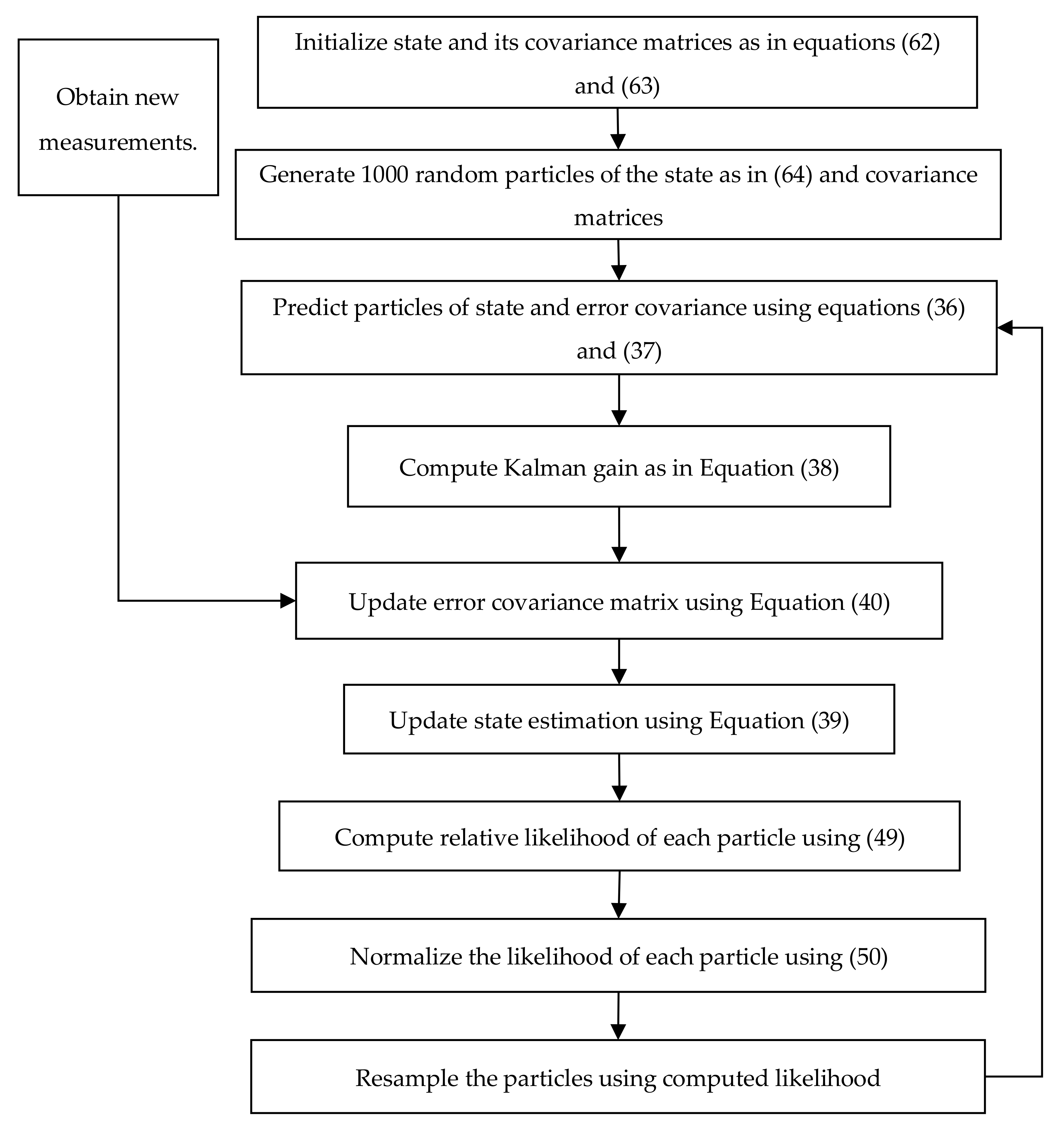
The particles of the target state vector for PFEKF and PFMGBEKF filters are generated by adding random noise to the initial state vector as in (58) for TST. Similarly, for SST the initial state vector is added with a column matrix of random numbers with four rows as in Equation (64) [22].
S S 0 | 0 j = S S 0 | 0 + r a n d n r a n d n r a n d n r a n d n r a n d n r a n d n T
Here, j represents the particle number and j = 1 ,   2 ,   3 ,   ,   1000 . The covariance matrix for each particle of the target state vector for PFEKF and PFMGBEKF filters are generated based on each particle generated.
It is not genuine to evaluate the performance of the algorithm on a run basis, as randomness exists in the experiment. Therefore, Monte Carlo simulation of 100 runs is performed for each filtering in MATLAB [6] for both SST and TST algorithms. The maximum (3σ) error acceptable in estimated range, course and speeds are 8% of true range, 3° and 1m/s, the root-mean-squared (RMS) (1σ) error allowed for the acceptance of the solution are 2.66% of true range, 1° and 0.33m/s respectively. The errors in the estimation of target parameters are root-mean-squared and the solution is assessed on the error acceptance levels mentioned above.
RMSE is nothing but root mean squared error and it is, in general, called standard deviation. It is implemented as follows. The difference between the true target parameter and the estimated target parameter is taken as error and it is squared. The mean of the squared error for all the 100 runs is then calculated and square rooted. This provides the RMSE of the estimated target parameters. Let i be the number of Monte Carlo runs and j be the total time in seconds for which the simulation is carried out. Then the error is mathematically given as Equation (65) and the RMSE as Equation (66).
E ij = true   target   parameter j estimated   target   parameter ij
RMSE j = mean E ij 2
The error in the estimated target parameters must be within the vicinity range of the weapon that has to be fired onto the target. The error in estimated target parameters is calculated based on Monte Carlo runs. Therefore, the RMSE values of the estimated target parameters are considered. With Monte Carlo simulations with 100 different noise sequences (maintaining same PDF), the outputs are root mean squared to obtain a single value. The acceptance criteria are chosen based on the weapon homing zone. The solution is said to be obtained only when the error in the estimated target parameters is less than the given values in acceptance criteria. Once the solution is obtained, the estimated target parameters can be used to release weapon onto the target.
The convergence time of the solutions for the three scenarios based on the above-mentioned acceptance criteria for 100 runs is tabulated in Table 2 for different filtering algorithms. In a Monte Carlo simulation, it is observed that UKF converges faster than other filters for BOT. Moreover, with single bearing measurement, the observer needs to follow S-maneuver, which can be avoided while using bearing measurements from two sensors.
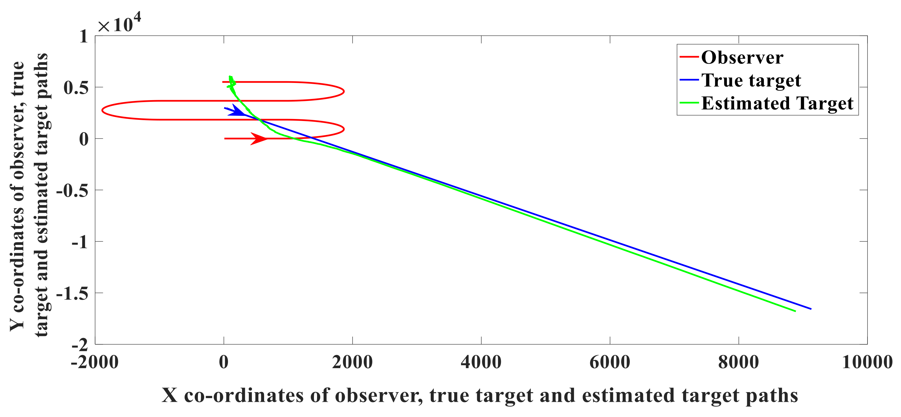
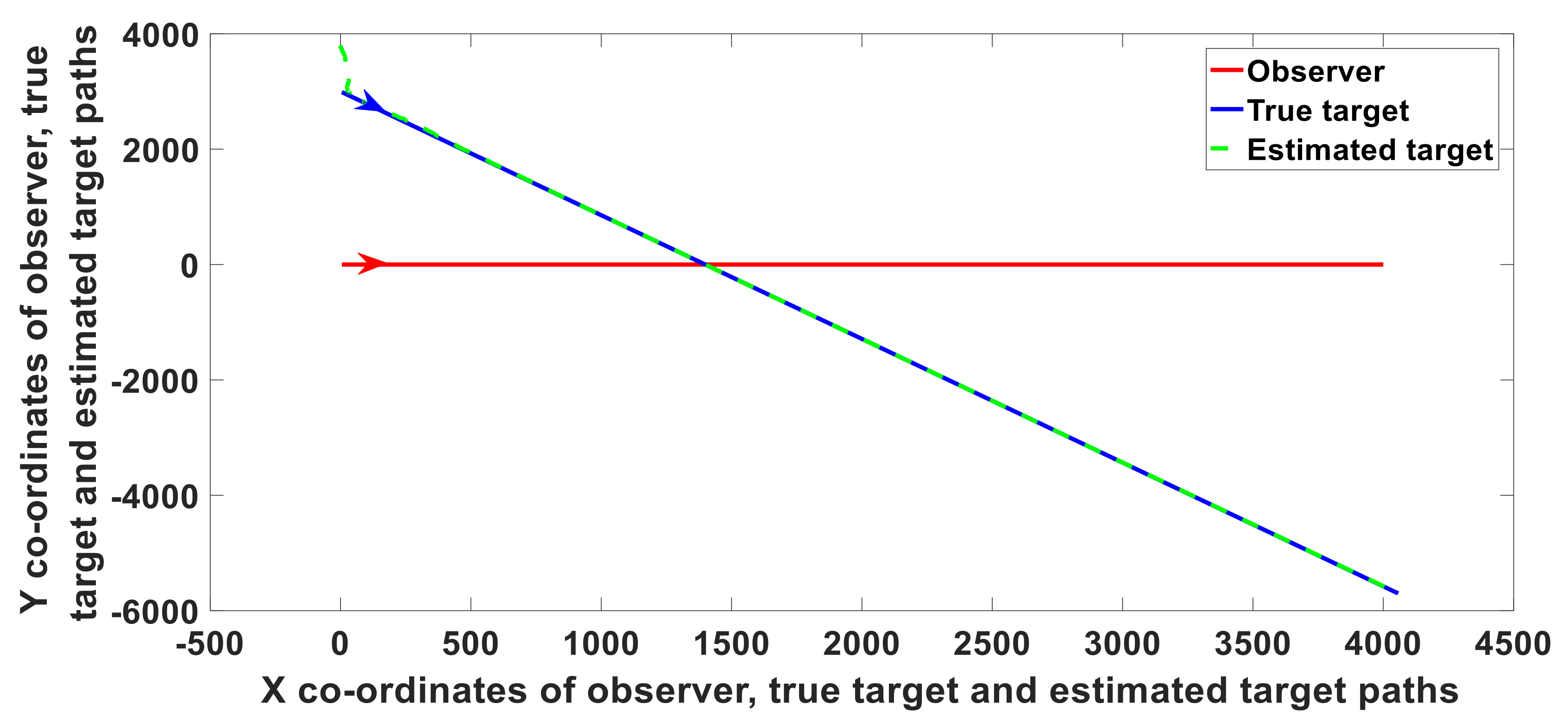
The simulation is carried out for 30 minutes. Results obtained with UKF for scenario 1 in Table 1 with SST and TST, are presented in Figure 3 and Figure 4 respectively. For SST, the observer needs to perform S-maneuver to obtain the observability of the process and hence to obtain a solution. With TST, the observability and solution are obtained even without observer maneuver as it uses bearing measurements from two sensors.
Table 3 gives the total convergence times of the solution with various filtering algorithms for TST. The solution is said to be converged if the acceptance criteria are achieved in all the three parameters at a time and the solution does not diverge for the rest of the simulation time. It can be observed from the table data that the solution convergence time is only for a short period with some of the scenarios and not for the entire simulated time for EKF. For scenario 2, the solution is converged from 227 to 447th second and then the solution diverged for the rest of the simulation time. The solution is not obtained for some of the scenarios with EKF. With MGBEKF, the same trend of solution-divergence persists. With UKF, the solution is obtained earlier than other filters for most of the scenarios. As shown in Table 3, UKF for scenario 1 has convergence time of 235 seconds whereas PFEKF and PFMGBEKF have convergence times of 337 and 237 seconds respectively. It can also be observed from Table 2 and Table 3 data that the convergence times for TST are obtained faster than SST.
As the measurements are taken from two different sensor arrays and both the measurements are nonlinearly related to the target state vector elements, the process nonlinearity will be very high. Therefore, sub-optimal nonlinear filters, EKF and MGBEKF, failed to give proper solutions. Particle filter deals with complete non-linearity and is suitable for highly nonlinear systems. However, to avoid the sample degeneracy problem it is combined with other filters and hence gives better results than EKF and MGBEKF.
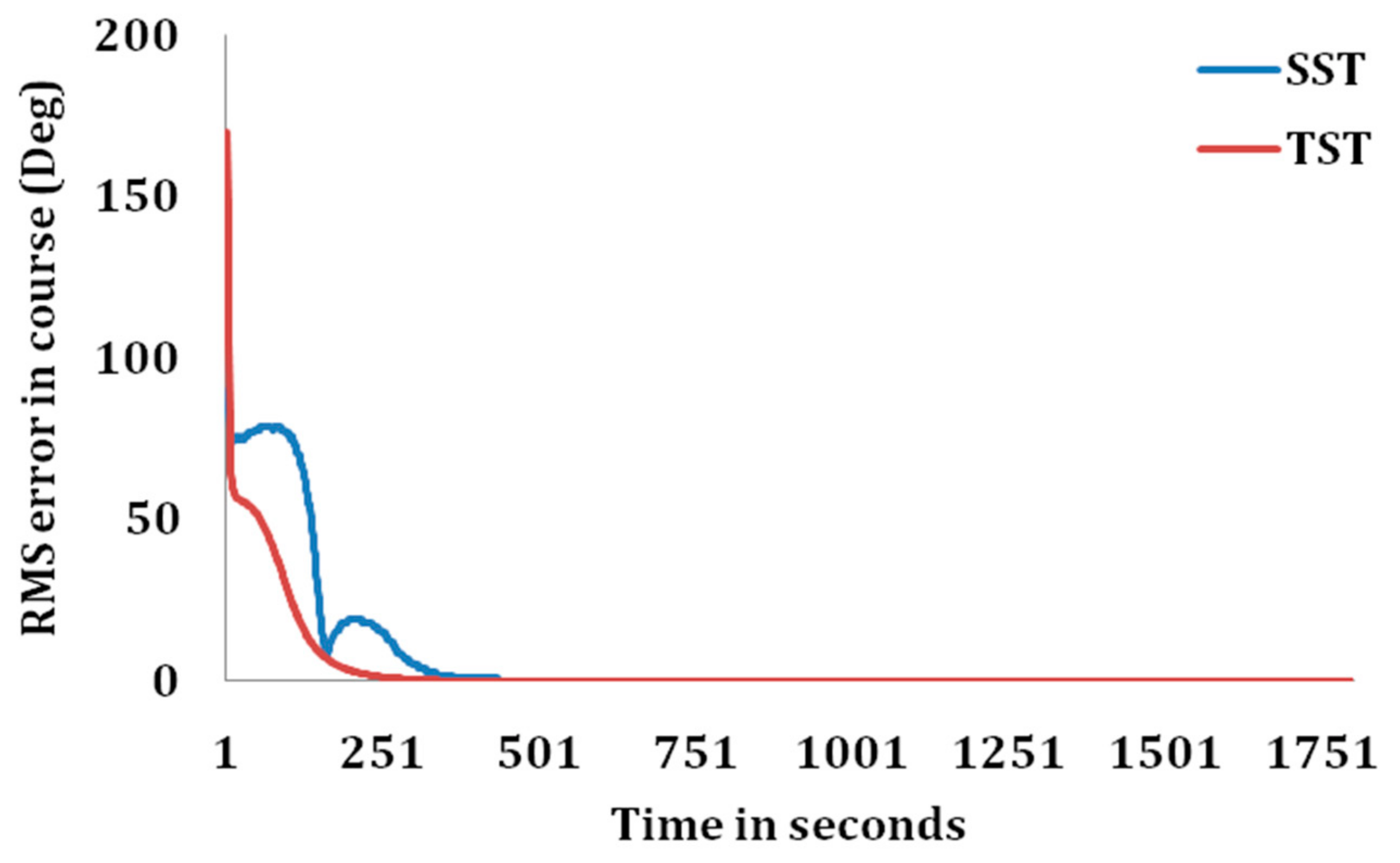
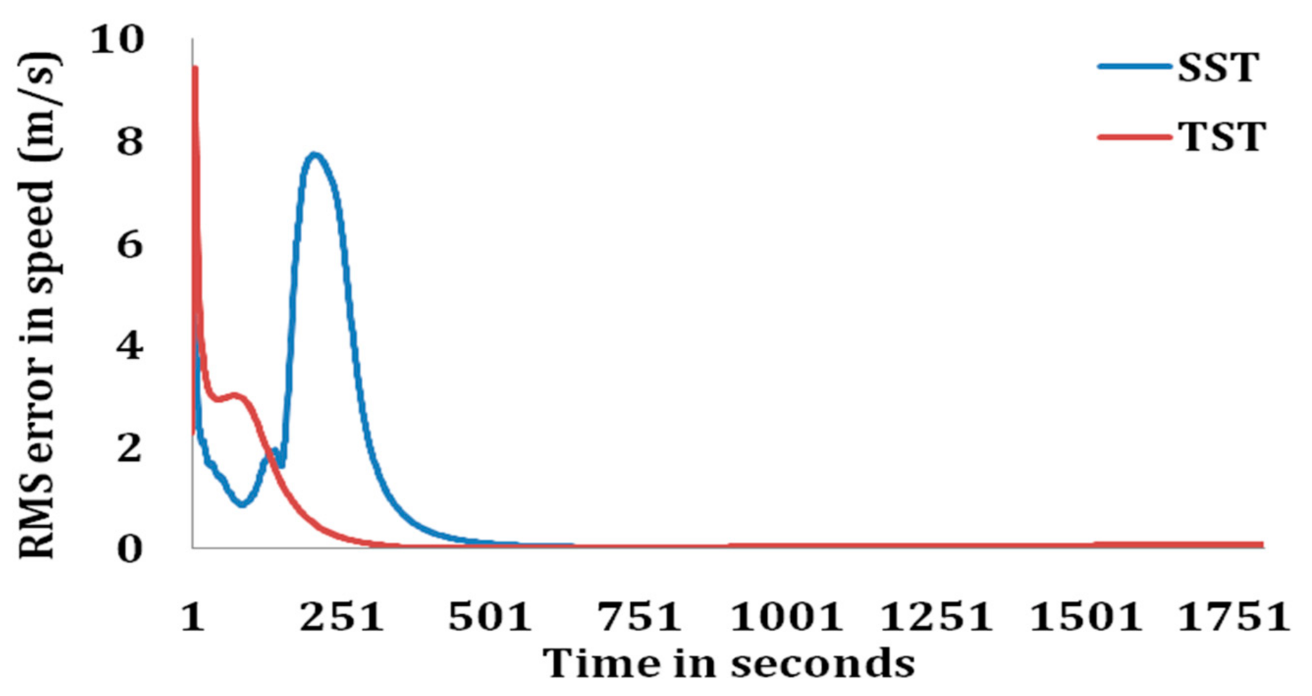
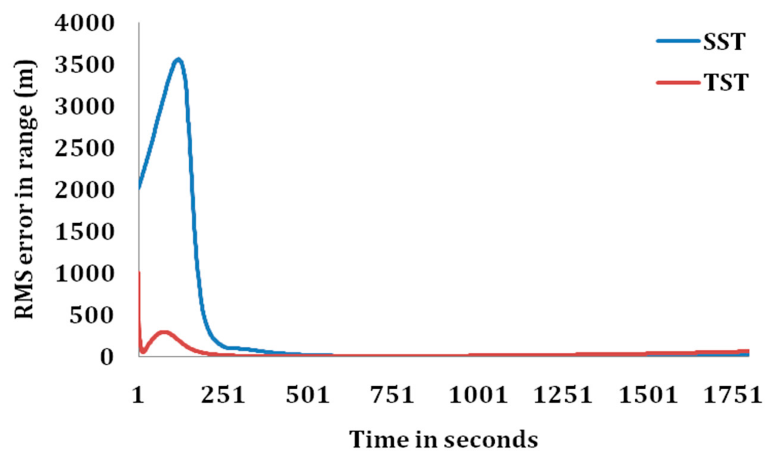
RMS errors in range, course, and speed estimates of the target are represented in Figure 5, Figure 6 and Figure 7. It can be observed from the figures that the RMS errors in estimated target parameters are less in case of TST than that with SST. RMS errors in estimated parameters are obtained within the acceptance criteria for TST much earlier than that of SST. However, as the range between observer and target increases, the RMS errors in estimated target parameters increases slightly for TST than that of SST.
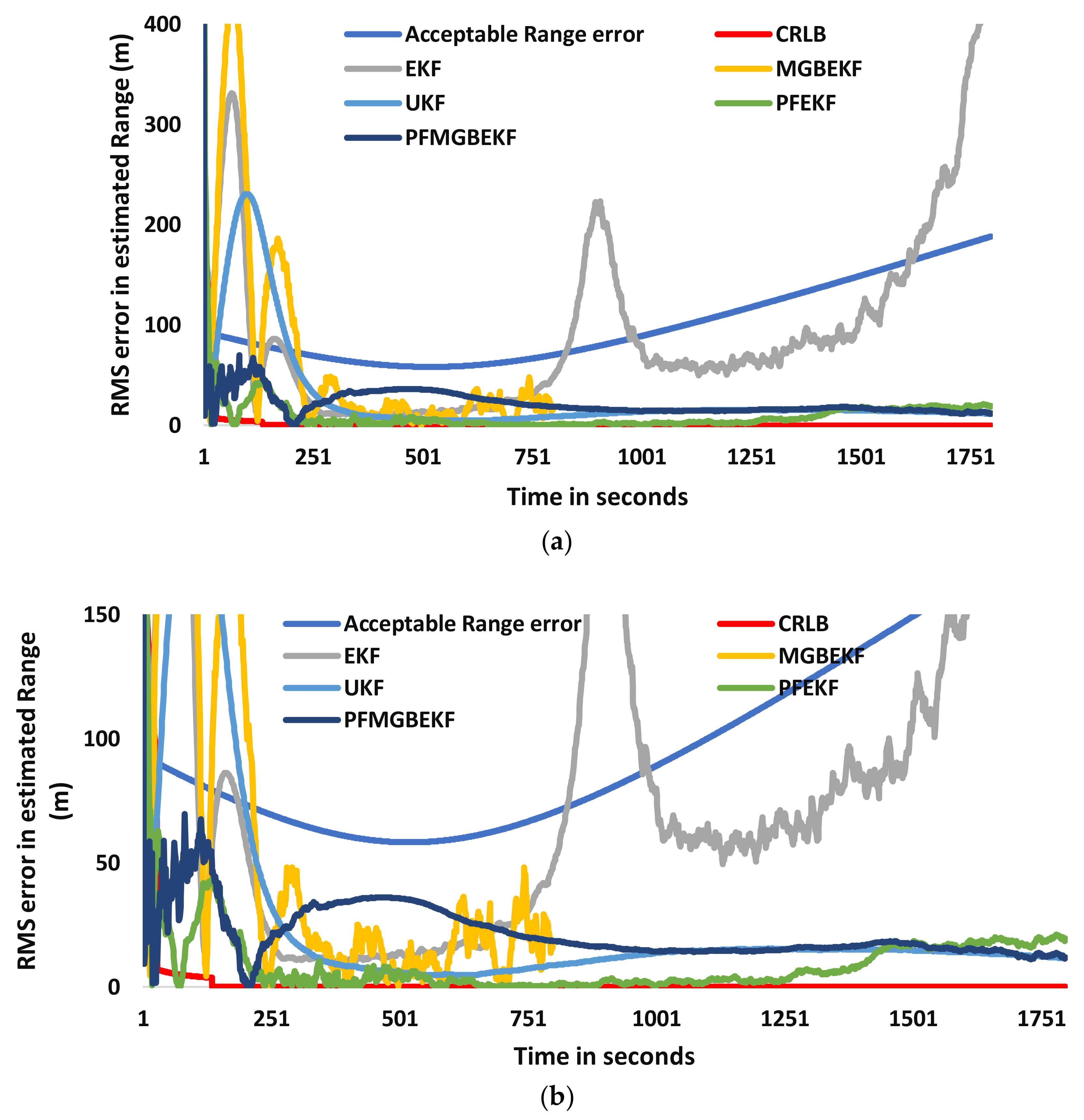
Figure 8 shows the acceptable error in range along with CRLB values for scenario 3, according to the acceptance criteria mentioned above, which is 2.667% of true range. RMS errors in the range of the target for different filters are also shown in Figure 8. It can be observed from the figure that lower RMS error is obtained earlier with PFEKF and PFMGBEKF filters than that of EKF, MGBEKF, and UKF filters. It can be seen from Figure 8b that the lowest RMS error is obtained with PFEKF. Though the error is below the acceptable error values, there is an effect of EKF that makes the error to vary in an unstable manner, which can be seen in the form of spikes in the plot. Similarly, with PFMGBEKF, the instability in error is reduced when compared to PFEKF.
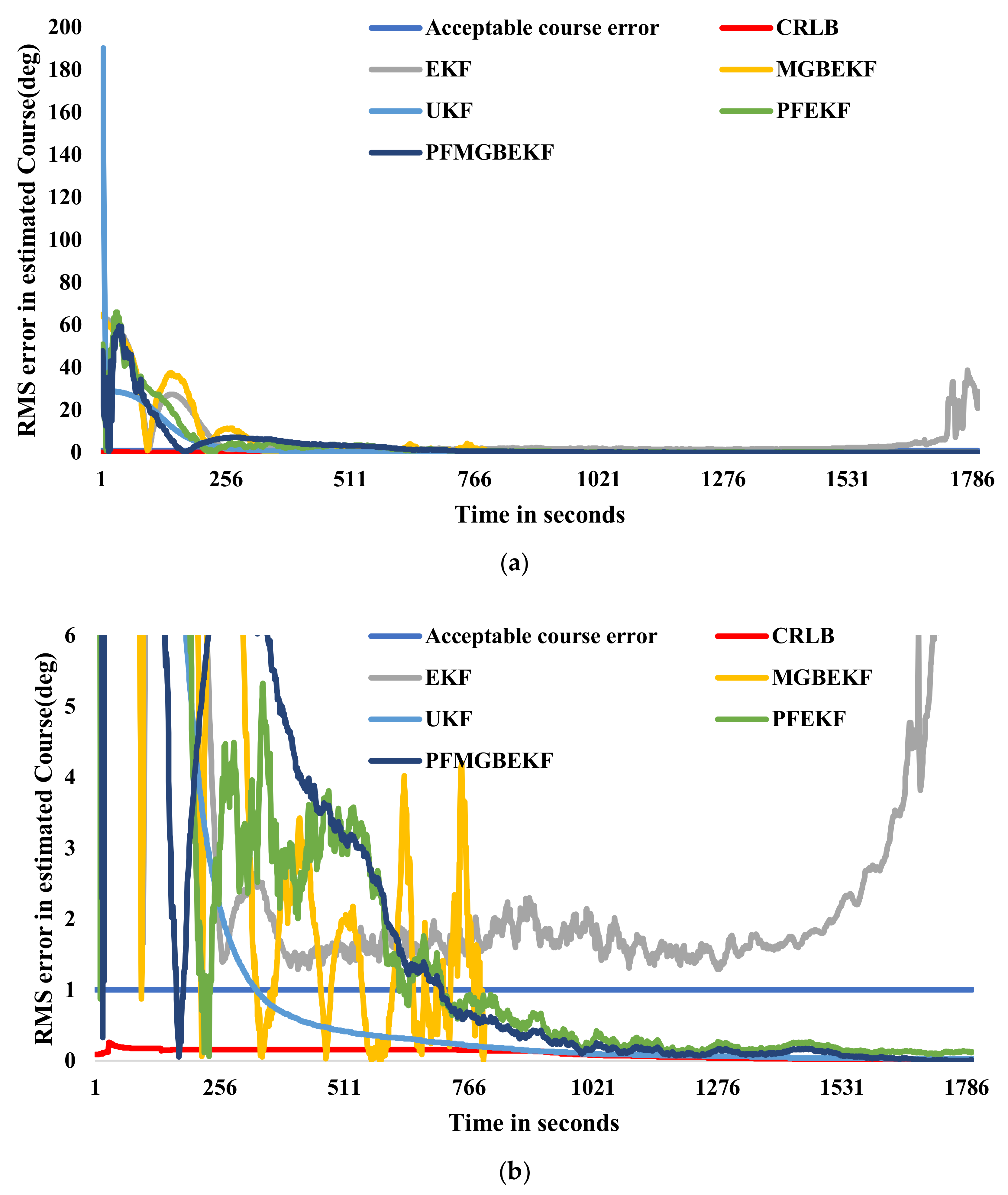
Figure 9 shows the acceptable error in the course for the same scenario 3, according to the acceptance criteria mentioned above, which is less than 1°. RMS errors in the course of the target for different filters are also shown in Figure 9. From Figure 9a, it can be observed that the error in the course is not obtained within acceptance criteria with EKF and MGBEKF. However, the fastest convergence in the target course was observed to be obtained with UKF, which can be seen from Figure 9b. PFEKF and PFMGBEKF also have convergence in the target course at 562 and 550 s respectively.
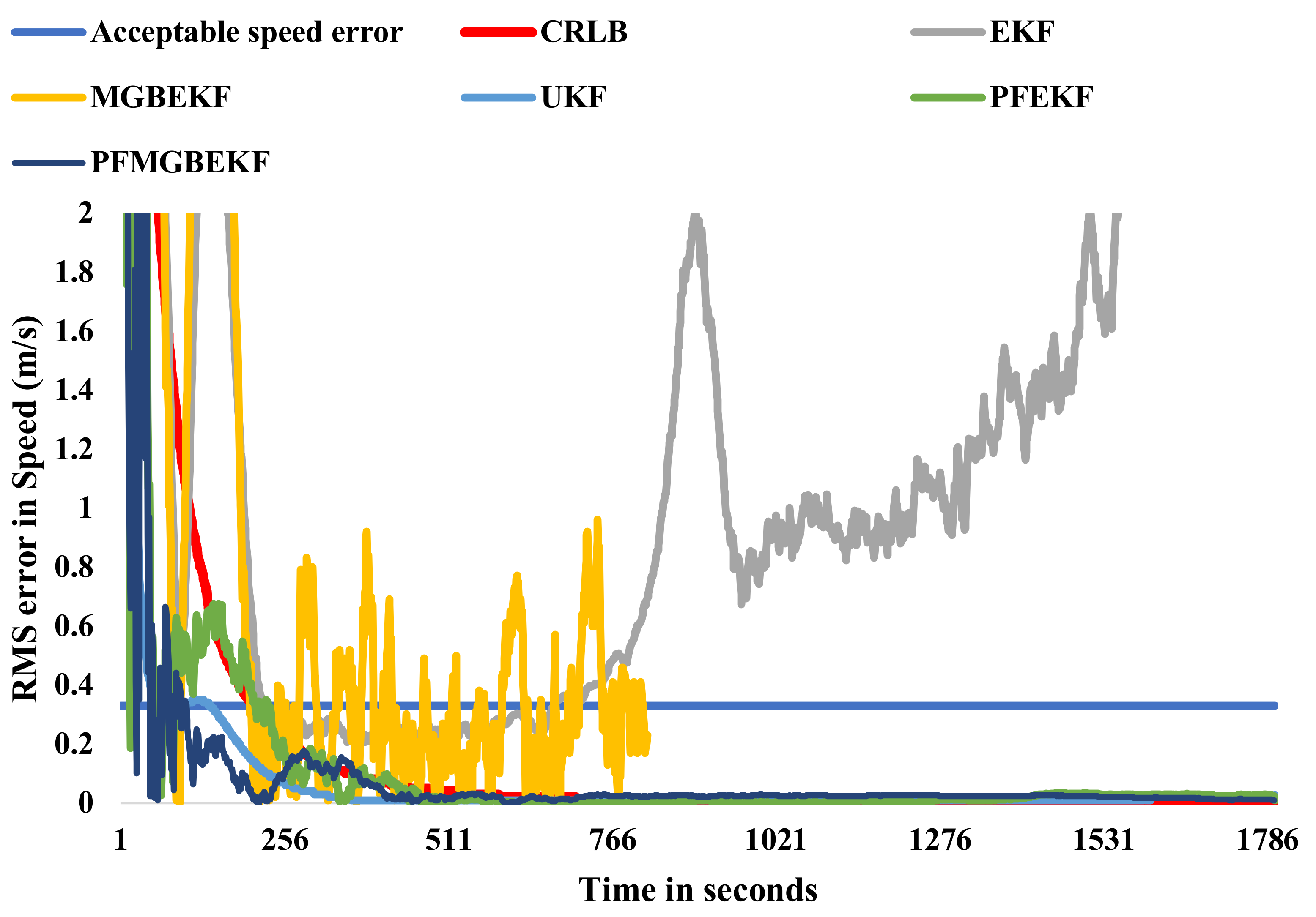
Figure 10 shows the acceptable error in speed for the same scenario 3, according to the acceptance criteria mentioned above, which is less than 0.33 m/s. RMS errors in the speed of the target for different filters are also shown in Figure 10. It can be observed from the figure that RMS error in speed with EKF and MGBEKF are varying in an unstable manner and are out of bounds after a certain time. With UKF, the convergence of speed error within acceptable criteria takes a shorter time than other filters and has a stable pattern. With PFMGBEKF, the lowest values in error are obtained. The overall convergence times were observed to be shorter for UKF than other filters and hence UKF performs well for TST than other filters.

4. Conclusions

In an underwater scenario, the observer and target are considered as submarines. Accordingly, scenarios are considered covering different target courses. SST and TST algorithms are considered for the performance evaluation concerning the convergence of the solution using different filters. Simulation is carried out and it is confirmed that TST generates the solution faster when compared to SST and even without observer maneuver. Hence, for passive target tracking, tracking with two bearing measurements is recommended. For TST, it was observed from simulated results that UKF provides a faster solution than other filtering algorithms.

Author Contributions

Conceptualization, K.J. and K.R.S.; Methodology, K.J. and K.R.S.; Software, K.J.; Validation, K.J. and K.R.S.; Formal analysis, K.J. and K.R.S.; Writing—original draft preparation, K.J. and K.R.S.; Writing—review and editing, K.R.S.; Supervision, K.R.S. All authors have read and agreed to the published version of the manuscript.

Funding

This research was funded by the Department of Science and Technology (DST) under the WOS-A scheme via a sponsored project: SR/WOS-A/ET-139/2017(G).

Acknowledgments

The authors would like to acknowledge DST, New Delhi, and President, Koneru Lakshmaiah Education Foundation (Deemed to be University) for their continuous support and encouragement.

Conflicts of Interest

The authors declare no conflict of interest.

References

  1. Nardone, S.C.; Lindgren, A.G.; Gong, K.F. Fundamental properties and performance of conventional bearings-only target motion analysis. IEEE Trans. Autom. Control 1984, 29, 775–787. [Google Scholar] [CrossRef]
  2. Lindgren, A.G.; Gong, K.F. Position and velocity estimation via bearing observations. IEEE Trans. Aerosp. Electron. Syst. 1978, 14, 564–577. [Google Scholar] [CrossRef]
  3. Aidala, V.J. Kalman filter behavior in bearings-only tracking applications. IEEE Trans. Aerosp. Electron. Syst. 1979, 15, 29–39. [Google Scholar] [CrossRef]
  4. Lindgren, A.G.; Gong, K.F. Properties of a bearings-only motion analysis estimator: An interesting case study in system observability. In Proceedings of the 12th Asilomar Conference on Circuits, System, and Computing, San Diego, CA, USA, 6–8 November 1978; pp. 265–272. [Google Scholar]
  5. Nardone, S.C.; Aidala, V.J. Observability criteria for bearings-only target motion analysis. IEEE Trans. Aerosp. Electron Syst. 1981, 17, 162–166. [Google Scholar] [CrossRef]
  6. Koteswara Rao, S. Pseudo-linear estimator for bearings-only passive target tracking. IEEE Proc. Radar Sonar Navig. 2001, 148, 16–22. [Google Scholar] [CrossRef]
  7. Wan, E.A.; Van Der Merwe, R. The unscented Kalman filter for nonlinear estimation. In Proceedings of the IEEE Symposium 2000 on Adaptive Systems for Signal Processing, Communication and Control, Lake Louise, AB, Canada, 1–4 October 2000; pp. 153–158. [Google Scholar] [CrossRef]
  8. Julier, S.J.; Uhlmann, J.K. A new extension of the Kalman filters to nonlinear systems. In Signal Processing, Sensor Fusion, and Target Recognition VI; International Society for Optics and Photonics: Bellingham, WA, USA, 1997; pp. 182–193. [Google Scholar]
  9. Koteswara Rao, S.; Raja Rajeswari, K.; Linga Murthy, K.S. Application of unscented Kalman filter for tracking underwater targets using bearings only measurements. In Proceedings of the IEEE International Conference on Soft Computing and Machine Learning for Signal Processing, Control, Power and Telecommunications, Bhubaneswar, India, March 2006; pp. 181–184. [Google Scholar]
  10. Koteswara Rao, S.; Raja Rajeswari, K.; Linga Murthy, K.S. Unscented Kalman filter with application to bearings-only target tracking. IETE J. Res. 2009, 55, 63–67. [Google Scholar] [CrossRef]
  11. Ristick, B.; Arulampalam, M.S.; Gordon, N. Beyond Kalman Filters–Particle Filters for Tracking Applications; Artech House, DSTO: Boston, London, 2004. [Google Scholar]
  12. Simon, D. Optimal State Estimation: Kalman, H∞ and Nonlinear Approximations; Wiley: Hoboken, NJ, USA, 2006. [Google Scholar]
  13. Bar-Shalom, Y.; Fortmann, T.E. Tracking and Data Association; Academic Press Inc.: New York, NY, USA, 1998. [Google Scholar]
  14. Koteswara Rao, S.; Raja Rajeswari, K.; Linga Murthy, K.S. Data fusion for underwater target tracking. IET Radar Sonar Navig. 2009, 4, 576–585. [Google Scholar] [CrossRef]
  15. Atherton, D.P.; Bather, J.A.; Briggs, A.J. Data fusion for several Kalman filters tracking a single target. IEEE Proc. Radar Sonar Navig. 2005, 152, 372–376. [Google Scholar] [CrossRef]
  16. Liu, G.; Wang, Y. Multi-Sensor Moving Target Tracking Using Particle Filter. In Proceedings of the IEEE International Conference on Robotics and Biomimetics, Sanya, China, 15–18 December 2007; pp. 668–673. [Google Scholar] [CrossRef]
  17. Yang, R.; Bar-Shalom, Y.; NG, G.W. Bearings-Only Tracking with Fusion from Heterogenous Passive Sensors: ESM/EO and Acoustic. J. Adv. Inf. Fusion 2017, 12. [Google Scholar]
  18. Lee, E.H.; Song, T.L. Multi-sensor track-to-track fusion with target existence in cluttered environments. IET Radar. Sonar Navig. 2017, 11, 1108–1115. [Google Scholar] [CrossRef]
  19. Dong, Y.; Zhang, G.; He, X.; Tang, J. Information Fusion in Networked Underwater Target Detection. In Proceedings of the IEEE OCEANS, Genoa, Italy, 18–21 May 2015; pp. 1–4. [Google Scholar] [CrossRef]
  20. Li, Y.; Zhao, Z. Passive Tracking of Underwater Targets Using Dual Observation Stations. In Proceedings of the International Bhurban Conference on Applied Sciences & Technology (IBCAST), Islamabad, Pakistan, 8–12 January 2019; pp. 867–872. [Google Scholar] [CrossRef]
  21. Kausar, J.; Koteswara Rao, S. Implementation of underwater target tracking techniques for Gaussian and non-Gaussian environments. Comput. Electr. Eng. 2020, 87, 106783. [Google Scholar] [CrossRef]
  22. Kausar, J.; Koteswara Rao, S. Extended Kalman Filter for Bearings-Only Tracking. Int. J. Eng. Adv. Technol. (IJEAT) 2019, 8, 637–640. [Google Scholar] [CrossRef]
  23. Li, T.; Bolić, M.; Djurić, P.M. Resampling Methods for Particle Filtering: Classification, implementation, and strategies. IEEE Signal Process. Mag. 2015, 32, 70–86. [Google Scholar] [CrossRef]
  24. Koteswara Rao, S. Bearings-Only Tracking. Observer Maneuver Recommendation. IETE J. Res. 2018. [Google Scholar] [CrossRef]
Figure 1. The observer with two arrays.
Information 11 00432 g001
Figure 2. Flow chart representing PFEKF algorithm.
Information 11 00432 g002
Figure 3. Target and observer paths with SST for scenario 1.
Information 11 00432 g003
Figure 4. Target and observer paths with TST for scenario 1.
Information 11 00432 g004
Figure 5. RMS error in range estimates of the target with SST and TST.
Information 11 00432 g005
Figure 6. RMS error in course estimates of the target with SST and TST.
Information 11 00432 g006
Figure 7. RMS error in speed estimates of the target with SST and TST.
Information 11 00432 g007
Figure 8. RMS error in range estimate of the target for scenario 3. (a) RMS error in range estimate of the target. (b) Expanded view of Figure 8a.
Information 11 00432 g008
Figure 9. RMS error in course estimate of the target for scenario 3. (a) RMS error in course estimate of the target. (b) Expanded view of Figure 9a.
Information 11 00432 g009
Figure 10. RMS error in speed estimate of the target.
Information 11 00432 g010
Table 1. Scenarios for the evaluation of algorithms.
ParameterScenario No.
123
Initial Range (m)300030003000
Initial Bearing (deg)000
Target Speed (m/s)121212
Observer Speed (m/s)888
Target course (deg)155145110
Observer course (deg)909090
Table 2. Convergence times of target parameters in seconds using the SST algorithm.
FilterScenario No.Target ParameterSimulation Time
RCSTC
EKF1273301330330462.82
2NCNCNCNC239.49
3339416339416408.42
MGBEKF1NCNCNCNC287.53
2NCNCNCNC371.97
3249321240321380.34
UKF1216216216216329.3
2244239329329345.6
3320338318338441.23
PFEKF1247247247247263.85
2249246245249122.39
3343434340434236.39
PFMGBEKF1273320269320398.29
2236337301337389.29
3270457288457228.24
R: Range; C: Course; S: Speed; TC: Total Convergence; NC: No Convergence.
Table 3. Convergence times of target parameters in seconds using the TST algorithm.
FilterS. NoTarget ParameterSimulation Time
RCSTC
EKF1155200–253;
347–442
213–257;
301–532
200–253;
347–442
301.81
2158–447227–447182–447227–447255.68
3109–148;
187–828
NC226–676NC441.86
MGBEKF118–676;
679–730
206–296;
377–401
159–357206–296;
386–410
1160.08
217–296NC124–296NC315.04
3218333–365;
465–485;
550–611;
655–675
206–246;
260–280
NC385.01
UKF1193235230235427.36
2175248221248430.81
3202333140333325.57
PFEKF1116337242337141.40
2119437259437159.59
3114713200713198.75
PFMGBEKF1116237150237436.61
21192561522561038.03
313071285712163.65
S. No: Scenario Number; R: Range; S: Speed; C: Course; TC: Total Convergence; NC: No Convergence.

