1. Introduction
The management of massive data represents a serious problem in image data clustering both in terms of memory allocation and execution times. In order to overcome this problem, it is necessary to reduce the size of the image, without producing information losses that affect the results of the clustering process. An idea to reduce the image size is to aggregate similar adjoint pixels into bins, using these bins as input data in the clustering process.
Bit-reduced fuzzy c-means (for short, brFCM) is an extension of the fuzzy c-means (for short FCM) algorithm [
1,
2] proposed in [
3] in order to cluster large images. The image is binned removing the least significant bits in the pixels and binning adjoining identical pixel; then, a weighted FCM is applied to the binned image considering as weight the number of pixels in each bin.
In [
4] brFCM is applied in very large (VL) image data clustering; the image is reduced by removing the least significant bits in the pixel values and binning adjoint pixel with identical grey level values; the weights are given by the number of pixels in each bin; the data assigned to the bin is the average of the pixel values of its pixels. The authors show that its performances are better than the ones of other FCM variations proposed in literature to cluster large and very large data.
An extension of the brFCM is proposed in [
5] in hotspot detection from massive event spatial datasets. The binning strategy was to reduce the spatial scale and aggregating in a bin data points included in a determined convex region in the map; a bin is given by the centroid of the event points included in that region and its weight is given by the number of data points located inside this region.
A serious problem in applying the brFCM algorithm to massive images is the difficulty in storing in memory the entire image for binning similar adjoint pixels.
To solve this problem in this research we propose a new image bit reduction FCM clustering algorithm, called FTbrFCM, for segmenting massive image datasets in which the brFCM algorithm is applied to images compressed via F-transform.
The fuzzy transform technique [
6] (for short, F-transform) is a consolidated method applied for lossy image compression [
6,
7,
8]. In particular, in [
7,
8] is proposed a F-transform image compression method in which the image s decomposed in blocks; each block is compressed via F-transform and the compressed image is obtained merging the compressed blocks. In [
9] the block F-transform image compression method is applied in image segmentation.
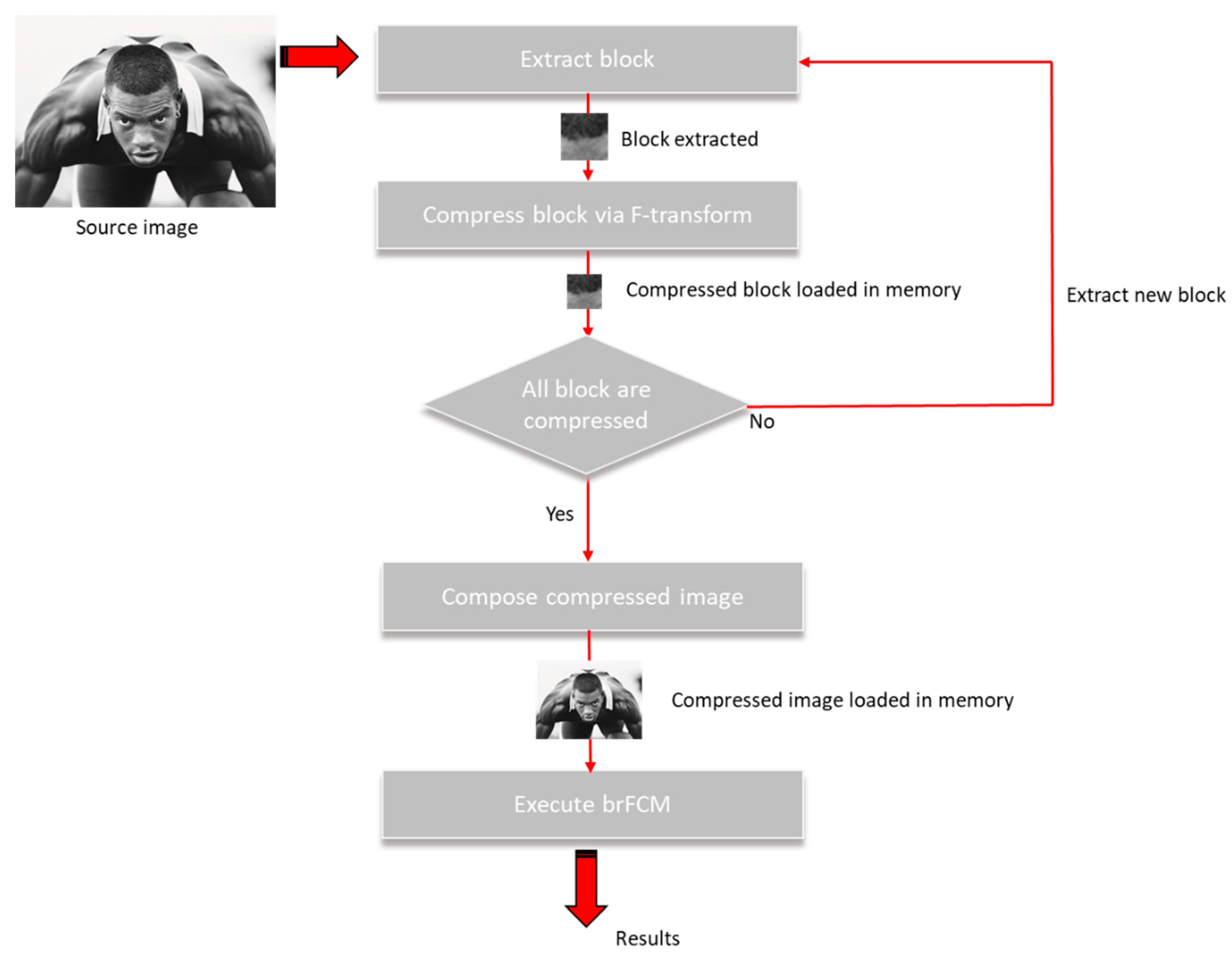
In FTbrFCM we apply this block F-transform image compression method to compress the image, then, the bit reduction method is executed to the compressed image, removing the least significant bits and merging adjoining identical pixels.
In this way, the whole image is not loaded in memory, but only some of its blocks; each block is compressed using the F-transform algorithm and, subsequently, the compressed image is recomposed in memory and the brFCM algorithm is applied.
In this way we obtain the following advantages:
- -
The clustering algorithm can be applied to the entire compressed image stored in memory;
- -
The runtime of the image segmentation algorithm is reduced, since it is applied on the compressed image;
- -
It is not necessary to remove the least significant bits in the pixels for bin the image, as the F-transform algorithm used to compress the image has already smoothed the image and the bins can be obtained spatially adjacent merging pixels with the same gray value.
The FTbrFCM algorithm is schematized in
Figure 1.
After the compressed image is constructed merging adjoint compressed blocks, the brFCM algorithm is executed aggregating in a bin identical adjoint pixels and then running the weighted FCM in which the weight of a bin is given by the number of pixels aggregated in it.
The results are given by C segmented images, where C is the number of clusters; the value assigned to a pixel in the ith segmented image is given by the membership degree of its bin to the ith cluster.
We test our algorithm on high resolution color images comparing the performances with the ones measured executing FCM on the source not compressed image.
This document is structured as follows: in
Section 2 the bi-dimensional F-transform concept and the block-wise F-transform image compression method are introduced; a detailed discussion of the bidimensional F-transform and its application in image compression is in [
6,
7,
8]. The brFCM algorithm is descripted in
Section 3. In
Section 4 the FTbrFCM algorithm is presented in detail. In
Section 5 are shown the results of comparison test applied in image. Final discussions are in
Section 6.
2. F-Transform Image Compression
Let [a, b] ⊂ R be a closed interval, n ≥ 2 and {x1, x2, …, xn} ⊂ [a, b] be a set of points called nodes, such that a ≤ x1 < x2 < … < xn ≤ b. The family of fuzzy sets A1, …, An: [a, b] → [0, 1] is a fuzzy partition of [a, b] if for every i = 1, 2, …, n the following conditions hold:
Ai(xi) = 1
Ai(x) = 0 if x ∉ (xi−1, xi+1), where x0 = a and xn+1 = b
Ai(x) is a continuous function on [a, b];
Ai(x) strictly increases on [xi−1, xi] and strictly decreases on [xi, xi+1];
∀ x ∈ [a, b] . A1(x) + A2(x) + … + An(x) = 1 (Ruspini condition).
The fuzzy sets {A1, …, An} are called basic functions. They form an uniform fuzzy partition of [a, b] if n ≥ 3 and for every i = 1, 2, …, n the following conditions hold:
- 6.
xi = a + h ∙ i, where h = (b − a)/(n + 1) (that is, the nodes are equidistant);
- 7.
Ai(xi − x) = Ai(xi + x) for every x in [0, h]
- 8.
Ai+1(x) = Ai(x − h) for every x in [xi, xi+1] and i = 1, 2, …, n − 1.
Let
f be a function continuous in [a, b] and let
P = {
p1, …,
pm} be a discrete set of points in [a, b] in which the function
f is known. We assume that the set
P of these points is sufficiently dense with respect to the fixed uniform fuzzy partition, that is for each
i = 1, …,
n there exists an index
j in {1, …,
m} such that A
i(
pj) > 0. Then we can define the
n-tuple {
F1, …,
Fn} as the discrete F-transform of
f with respect to {A
1, A
2, …, A
n}, where each
Fi is given by:
for
k = 1, …,
n. Now we define the discrete inverse F-transform of
f with respect to {A
1, A
2, …, A
n} to be the following function defined in the same points
p1, …,
pm of [a, b]:
The (2) approximate the function
f in the interval [a, b] (cfr. [
5], Theorem 18).
2.1. F-Transforms in Two Variables
The discrete direct and inverse fuzzy transforms of a function f continuous in [a, b] can be extended to functions in two variables. Assume that our universe of discourse is the rectangle [a, b] × [c, d] and let m,n ≥ 2, {x1, x2, …, xm} ⊂ [a, b] be a set of nodes in [a, b] and {y1, y2, …, yn} ⊂ [c, d] be a set of nodes in [a, b], such that x1 ≤ a < x2 < … < xm ≤ b and y1 ≤ c < … < yn ≤ d. Furthermore, let A1, …, Am: [a, b] → [0, 1] be a fuzzy partition of [a, b] and B1, …, Bn: [c, d] → [0, 1] be a fuzzy partition of [c, d].
Let f be a function continuous in [a, b] × [c, d] known in a discrete set of points (pj,qj) ∈ [a, b] × [c, d], where i = 1, …, M and j = 1, …, N, P = {p1, …, pM} sufficiently dense with respect to {A1, …, Am} and Q = {q1, …, qN} sufficiently dense with respect to {B1, …, Bn}.
Then, generalizing the Equation (1), we can define the discrete F-transform matrix of
f [
Fkl], with respect to {A
1, …, A
m} and {B
1, …, B
n} with components
k = 1, …,
m and
l = 1, …,
n:
By extending Equation (2) to the case of two variables, we define the discrete bi-dimensional inverse F-transform of
f with respect to {A
1, A
2, …, A
n} and {B
1, …, B
m} to be the following function defined in the same points (
pi,
qj) in [a, b] × [c, d], with
i in {1, …,
N} and
j in {1, …,
M}, as:
The inverse F-transform (4) approximate the bidimensional function f in [a, b] × [c, d].
2.2. F-Transforms in Two Variables for Image Compression
Let I(x,y) an image function discretized in a digital gray M × N image composed of M × N pixels with coordinates (pi,qj) ∈ {1, …, M} × {1, …, N}. For brevity of notation, we put pi = i, qj = j and [a, b] × [c, d] = [1, N] × [1, M].
The matrix I is divided in submatrices of identical size MC × NC called blocks, where MC < M, NC < N, MC is a divisor of M and NC is a divisor of N. The image I is then composed of (MC × NC)/(M × N) blocks of equal size MC × NC.
Each block is composed of MC × NC pixels with coordinates (pi,qj) ∈ {1, …, MC } × {1, …, NC }. For brevity of notation, we put pi = i, qj = j and [a, b] × [c, d] = [1, MC] × [1, NC].
Let A1, …, Am: [1, MC] → [0, 1] be a fuzzy partition of [1, MC] with mC < MC and let B1, …, Bn: [1, NC] ⭢ [0, 1] a fuzzy partition of [1, NC] with nC < NC.
Each block of sizes M
C × N
C is compressed in a block of sizes m
C × n
C via the discrete bi-dimensional F-transform [
FklC] with components given by:
for each
k = 1, …,
mC and
l = 1, …,
nC. As above, naturally we do in such a way that the set{1, …, M(C) (resp., {1, …, N(C)})} is sufficiently dense to the fuzzy partition of the basic functions {A
1, …, A
m(C)} defined (resp., {B
1, …, B
n(C)}) in the interval [1, M(C)] (resp., [1, N(C)]) considered.
The parameter ρ: = (mC∙× nC)/(MC × NC) is the compression rate of the block.
Afterwards, we decode the compressed blocks via the discrete inverse F-transform
:{1, …, M(C)} × {1, …, N(C)} → [0, 1] defined as:
which approximates I
C with arbitrary precision.
The tests conducted in [10
14] have shown that the best performances are obtained by using a symmetric fuzzy partition of [1, M
C] whose fuzzy sets A
1, …, A
m(C):[1, M
C] → [0, 1]] are defined as
where
k =1, 2, …,
mC, h = (M
C − 1)/(m
C + 1), x
0 = 1 and x
mC + 1 = m
C, and by using a symmetric fuzzy partition of [1, N
C] whose fuzzy sets B
1, …, B
nC:[1, N
C] → [0, 1] are defined as:
where
l = 1, 2, …,
nC, s = (N
C − 1)/(n
C +1), y
0 = 1 and x
nC + 1 = n
C.
The compressed image Iρ of I obtained using the compression ratio ρ is constructed merging the compressed blocks where each compressed block is given by the direct F-transform matrix [FklC] calculated by (5).
Algorithm 1 shows in pseudocode the block F-transform image compression algorithm.
| Algorithm 1. Block F-Transform Image Compression. |
| Input: | Source Image I |
| Output: | Compressed image Iρ |
| 1 | Set MC,NC,nC,mC where ρ := mC∙nC / MC NC |
| 2 | Set the basic functions A1, A2, …, An as in (7) and B1, B2, …, Bn as in (8) |
| 3 | For each block IC |
| 4 | For k = 1 to mC |
| 5 | For l = 1 to nC |
| 6 | Numkl := 0 // Numerator of the Ftransform component (5) |
| 7 | Denkl := 0 // Denominator of the Ftransform component (5) |
| 8 | For i = 1 to MC |
| 9 | For j = 1 to NC |
| 10 | Numkl := IC(i,j)∙Ak(i) Bl(j) |
| 11 | Denkl := Ak(i) Bl(j) |
| 12 | Next j |
| 13 | Next i |
| 14 | FklC := Numkl / Denkl // Ftransform component (5) |
| 15 | Next l |
| 16 | Next k |
| 17 | Next block |
| 18 | Merge the compressed block to obtain the compressed image Iρ |
| 19 | Store the compressed image Iρ |
The compressed image Iρ can be decompressed dividing it in MC × NC blocks and decoding every block in a MC × NC block by (6); finally, the decoded blocks are merged to form the decompressed image.
3. The brFCM Algorithm
Let X = {x1, …, xN} ⊂ Rn be a set of data Np data points: each data point xj = (xj1, …, xjn) is a vector in the space Rn.
FCM is a partitive fuzzy clustering algorithm aimed to find as set of points in Rn the set of C fuzzy cluster centers V = {v1, …, vC} where vi = (vi1, …, vjn) (i = 1, …, C). The C × Np partition matrix U with components uij i = 1, …, C; j = 1, …, Np give the membership degree of the jth data point to the ith cluster.
FCM find
V and
U minimizing the following objective function:
where d
ij =
is the Euclidean distance between
vi and
xja.
The parameter γ ∈ [1, +∝) is called fuzzifier parameter; it determines the fuzziness degree of the fuzzy partition. (a constant which affects the membership values and determines the degree of fuzziness of the partition).
By applying the Lagrange multipliers, and considering the constraints:
are obtained for
U and
V the following solutions
and
FCM is an iterative algorithm in which initially the membership degrees (or the cluster centers) are assigned randomly; in any cycle the cluster centers and the membership degrees are calculated via (12) and (13). The algorithm stops after
t iterations if:
where
ε > 0 is a parameter assigned a priori to stop the iteration process and
The pseudocodes of the FCM is given in Algorithm 2.
| Algorithm 2. FCM. |
| Input: | Input Dataset D with Np Data Points |
| Output: | Partition matrix U and cluster centers V |
Set γ, ε, C Initialize randomly the partition matrix U Repeat Calculate vi, i = 1, …, C by using Equation (12) Calculate uij, i = 1, …, C j = 1, …, Np by using Equation (13) Until
|
A variation of the FCM algorithm is the weighted FCM (wFCM) algorithm [
10] in which a weight defines the influence of the data point to the solutions; data points with higher weights influence the determination of location of the cluster centers more than the others.
We can consider FCM a special case of wFCM where wj = 1 for each j = 1, …, Np, in which each data point influences the determination of cluster centers in the same way.
wFCM minimize the following objective function:
Using the Lagrange multipliers, and considering the constraints (10) and (11), are obtained for the cluster centers the solutions:
The solutions obtained for the membership degrees are given by (13).
The pseudocode of wFCM is shown in Algorithm 3.
| Algorithm 3. WFCM. |
| Input: | Input dataset D with NP data points |
| Output: | Partition matrix U and cluster centers V |
Set γ, ε, c Initialize randomly the partition matrix U Repeat Calculate wj, j = 1, …, Np by using a weight function w(xj) Calculate vi, i = 1, …, C by using Equation (17) Calculate uij, i = 1, …, C; j = 1, …, N by using Equation (13) Until
|
A density-based wFCM was proposed in [
11] for reducing the size of the input dataset. In [
12,
13] two weighted FCM algorithms are used for image segmentation. In [
14] a wFCM algorithm is applied to solve the Source Location problem.
The brFCM algorithm is proposed in [
3] to handle massive datasets. It uses a wFCM algorithm in which the weight is given by the number of data points merged in a bin.
The pseudocode of brFCM is shown in Algorithm 4.
| Algorithm 4. BRFCM. |
| Input: | Input dataset D with Np data points |
| Output: | Partition matrix U and cluster centers V |
Set γ, ε, c Bin the dataset in Np quantization bins Assign the weight wj, j = 1, …, Np as the number of data points merged in a bin Initialize randomly the partition matrix U Repeat Calculate vi, i = 1, …, C by using Equation (17) Calculate uij, i = 1, …, C; j = 1, …, N by using Equation (13) Until
|
5. Test Results
The FTbrFCM is applied to a set about 200 color high-resolution images of paintings by famous painters in the Google Art & culture web page (
https://artsandculture.google.com); the mean resolution of these images is of 10
8 pixels. Each image is decomposed in the three bands R, G and B, then, FTbrFCM is executed on the image in each band. The Xie-Beni validity index [
15] is used to find the optimal number of clusters.
We apply FTbrFCM on the image on each band by using various compression rates. We execute FTbrFCM on an Intel core I5 3.2 GHz processor.
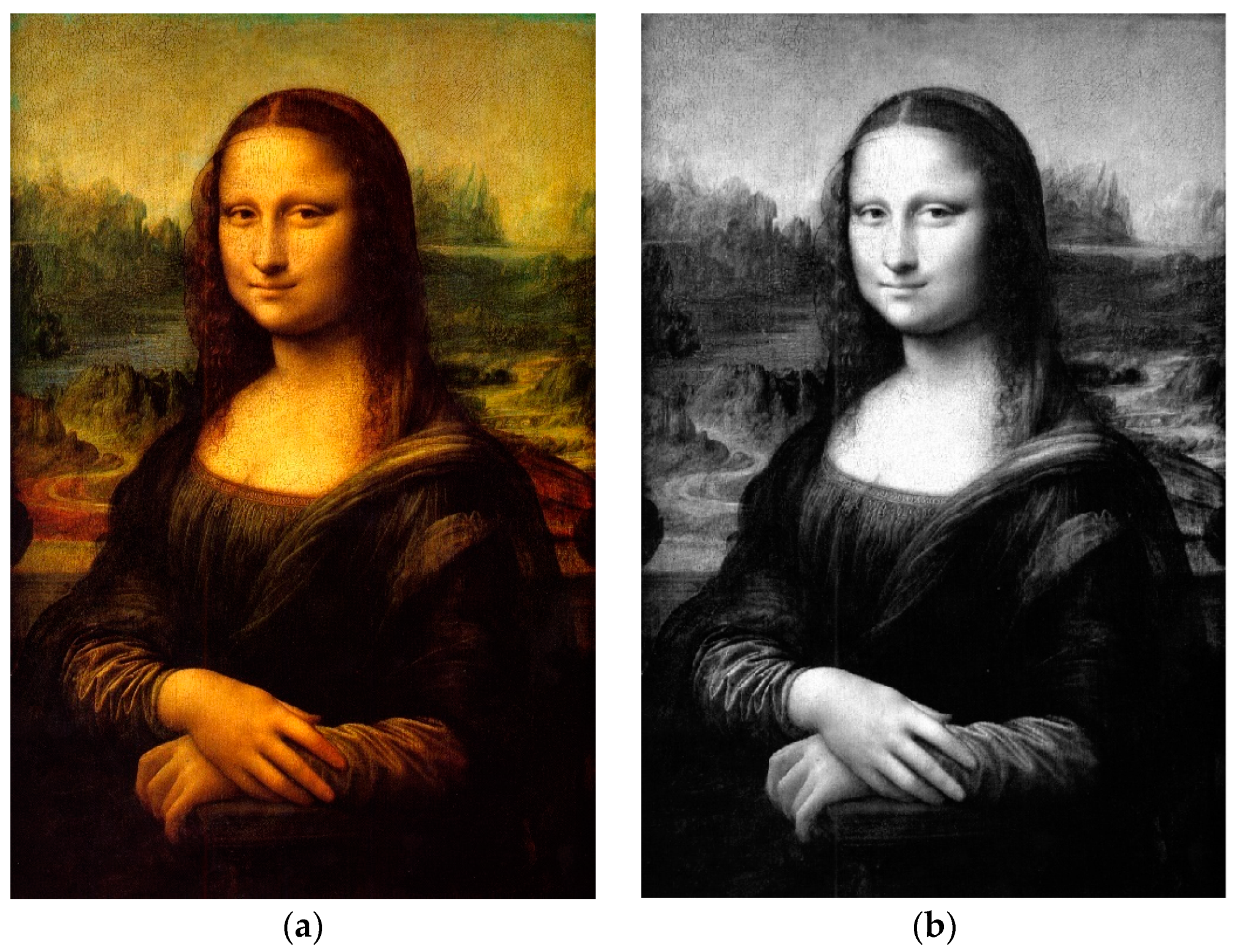
For brevity we present the detailed results obtained for the color images Mona Lisa, which represents the homonymous oil painting by Leonardo da Vinci preserved in the Louvre, and Sunflowers, which represents the Van Gogh’s the painting on canvas, Vase with 15 Sunflowers, preserved at Van Gogh Museum
In
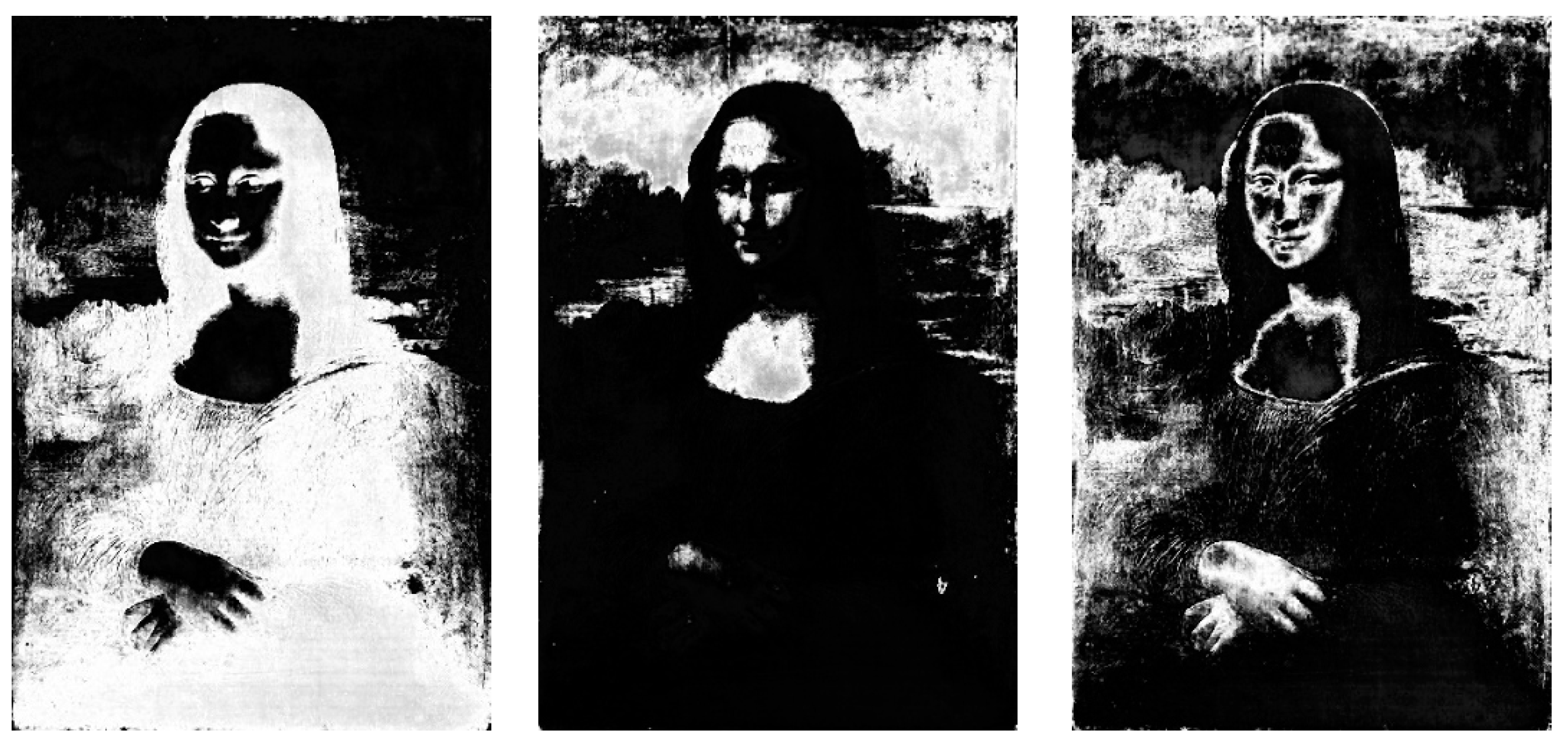
Figure 2a–d is shown the high-resolution image Mona Lisa decomposed in the three band R, G and B.
The images in the three bands are been compressed and segmented setting C = 3 clusters.
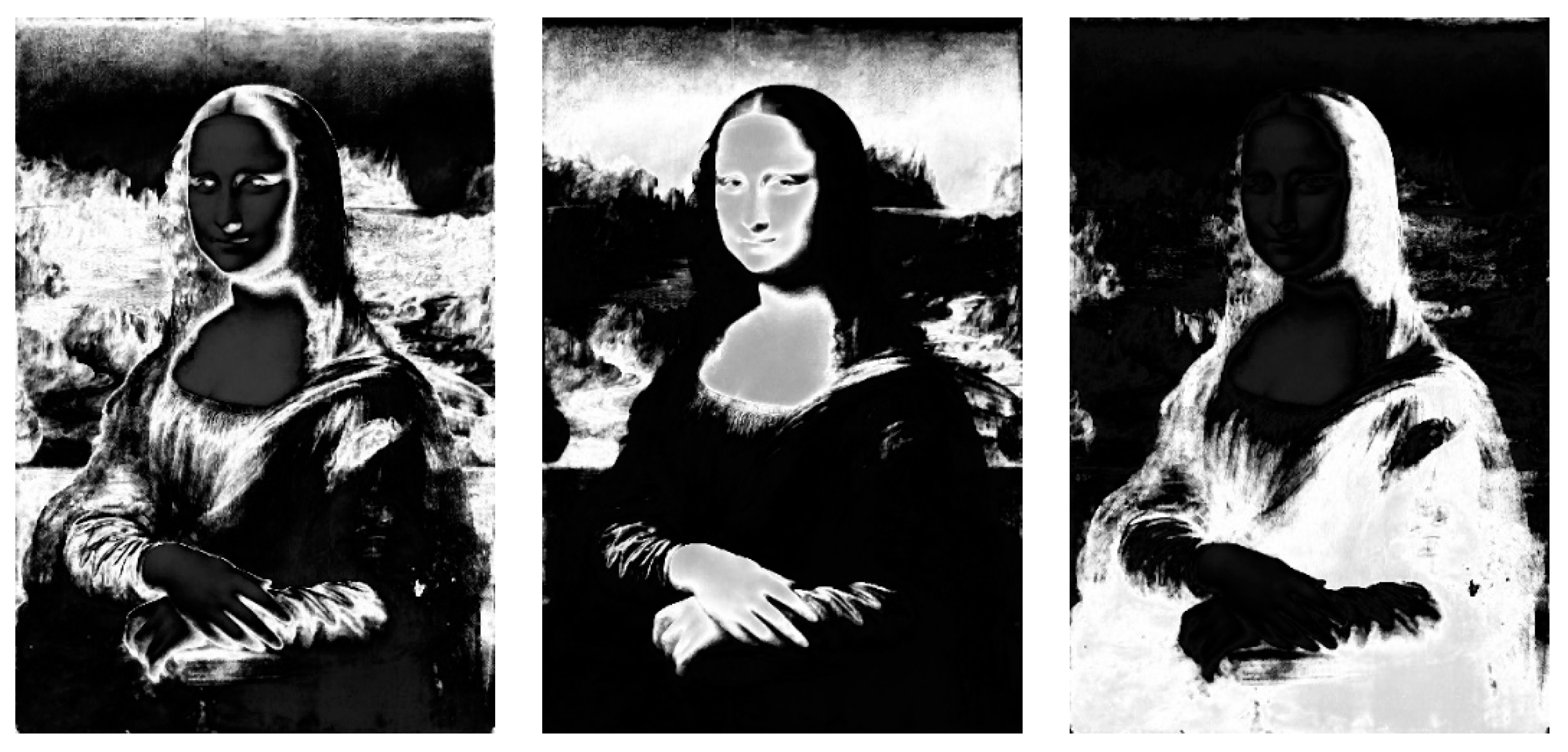
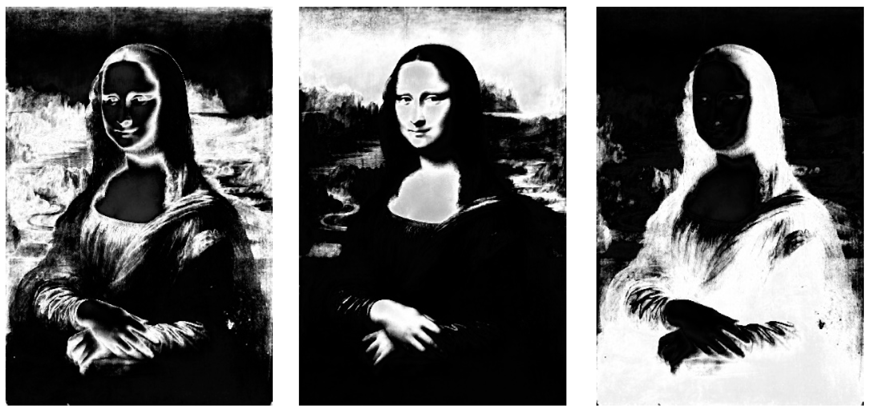
Figure 3,
Figure 4 and
Figure 5 show, respectively, the segmented images obtained in the bands R, G and B, compressing the original image with a compression rate
ρ = 0.25, obtained compressing each block 4 × 4 in a block 2 × 2.
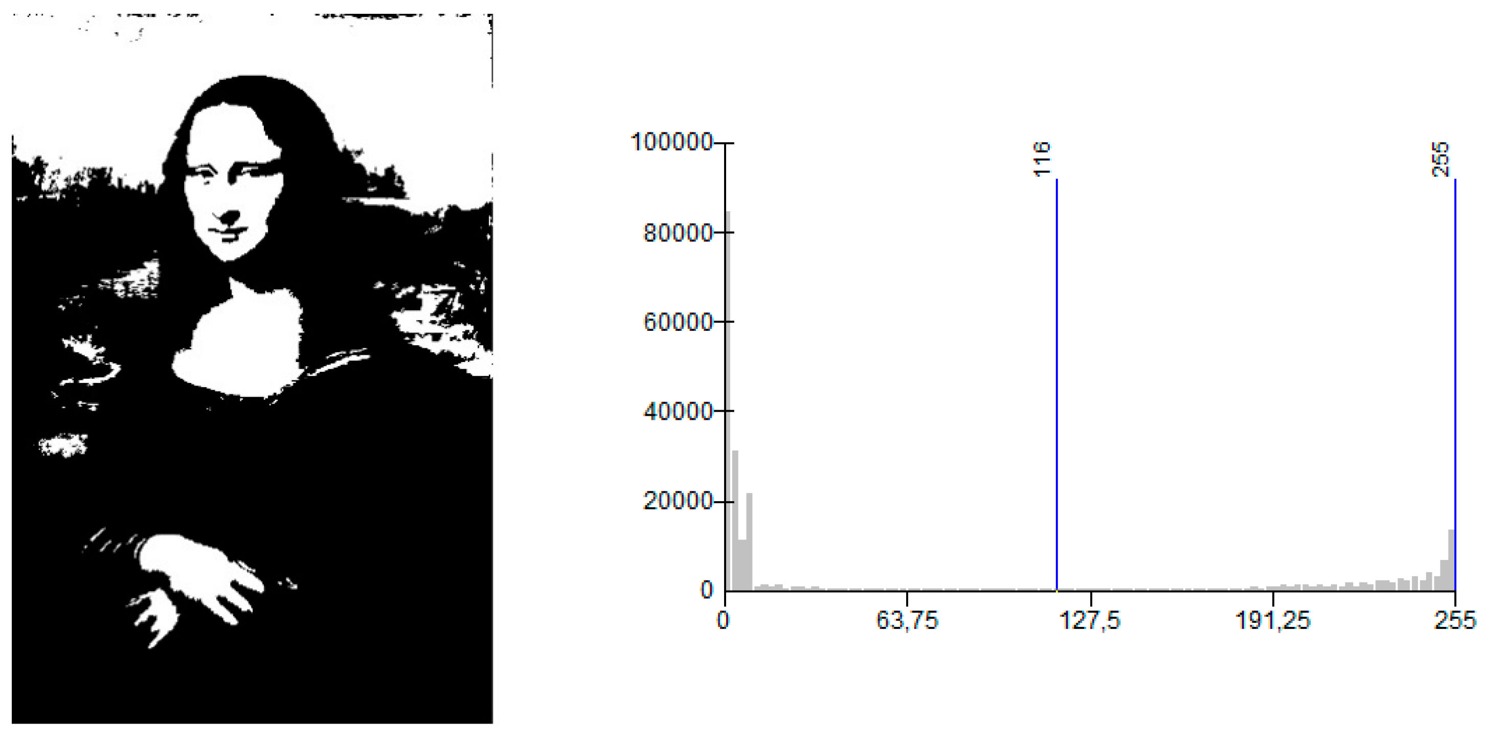
A segmented image can be subsequently processed to be classified. As an example, the binary image in
Figure 6 show the results of the classification of the second segmented image in the G band and the pixel values frequency histogram used to classify the pixels.
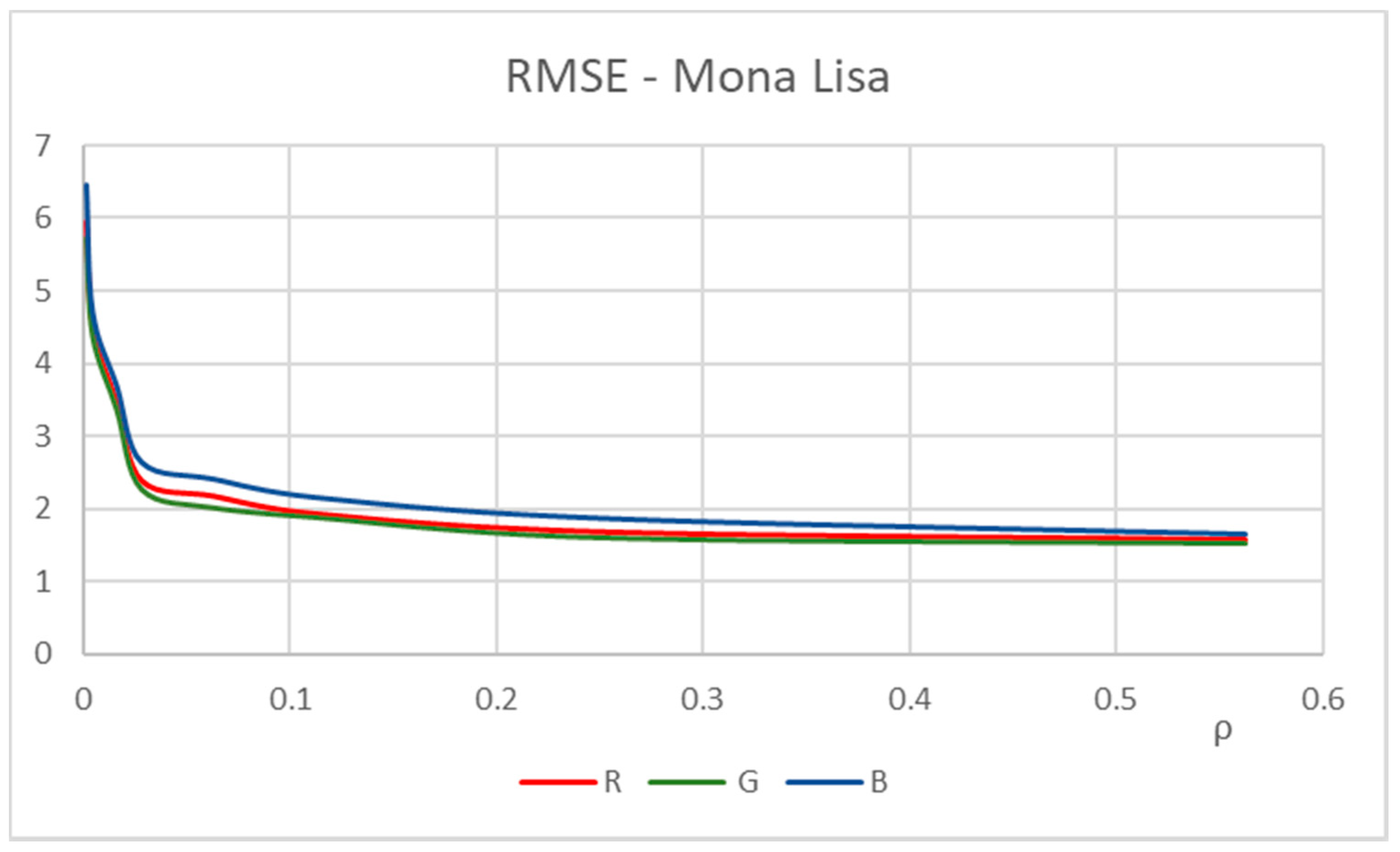
We calculate the RMSE index of the segmented image obtained in a band with respect to the correspondent segmented image obtained applying FCM on the source image in that band. To perform these measures, we decompress the segmented images obtained by executing the FTbrFCM algorithm using the bidimensional inverse F-transform.
In
Table 1 are shown the RMSE measures obtained in each band changing the compression rate.
The trend of RMSE varying the compression rate is shown in
Figure 7.
This results show that for not high compressions (ρ greater than 0.016), the RMSE index is less than 3, i.e., the average difference of the pixel values between the segmented image obtained using the FTbrFCM algorithm and the corresponding one obtained using the FCM algorithm is less than 3, therefore the loss of information due to the compression of the source image can be considered acceptable. In fact, if the mean square error obtained is less than 3 the average absolute difference between the membership degree of a pixel to the cluster obtained with the two algorithms is less than 3/255 ≈ 1.2 × 10⁻² and the loss of information can be neglected. For strong compressions (ρ < 0.1), however, the RMSE value rises rapidly and the average differences between the membership degree values assigned to each pixel become significant.
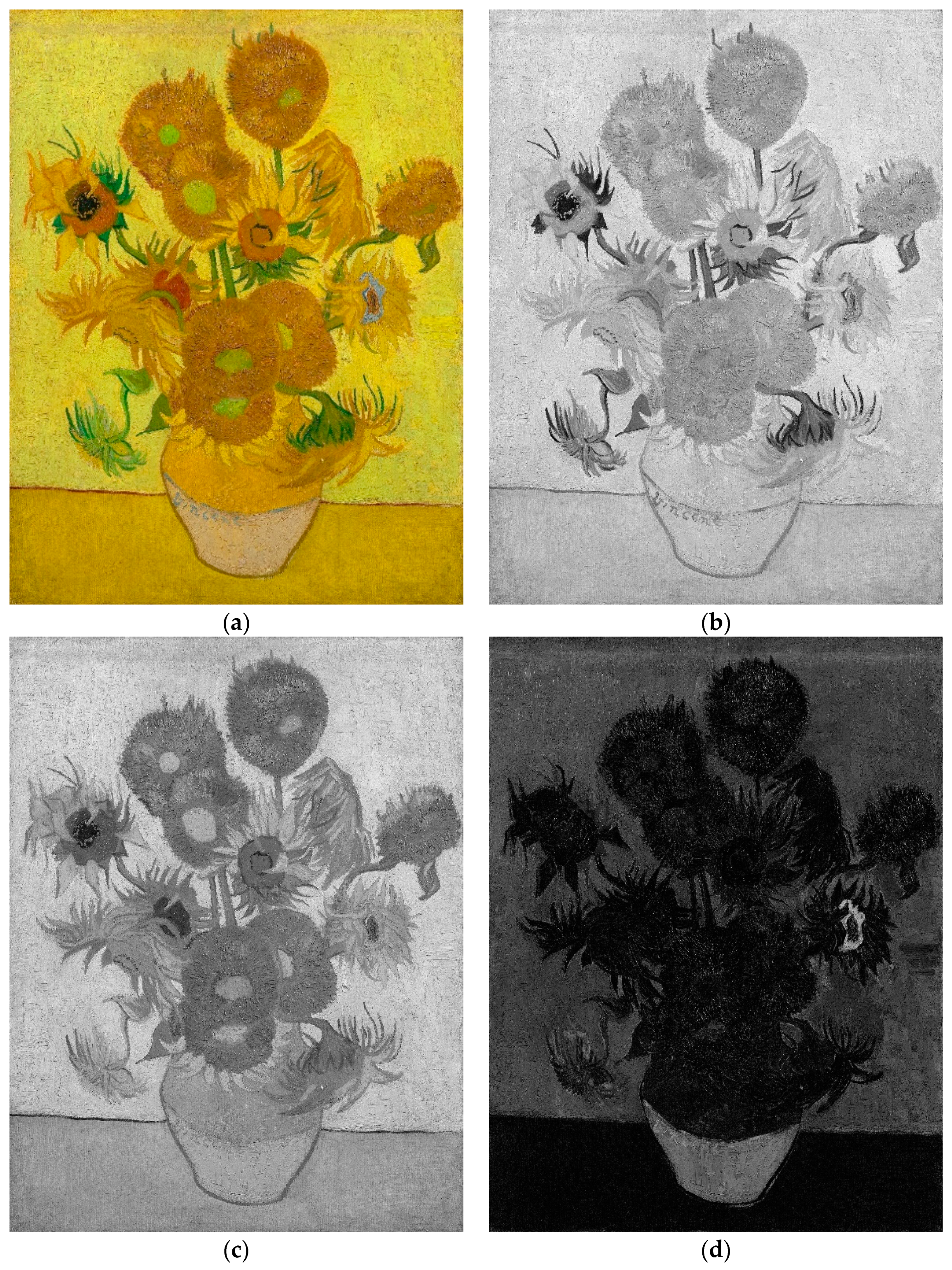
In
Figure 8a–d are shown the image Sunflowers and its decomposition in the three bands R, G and B.
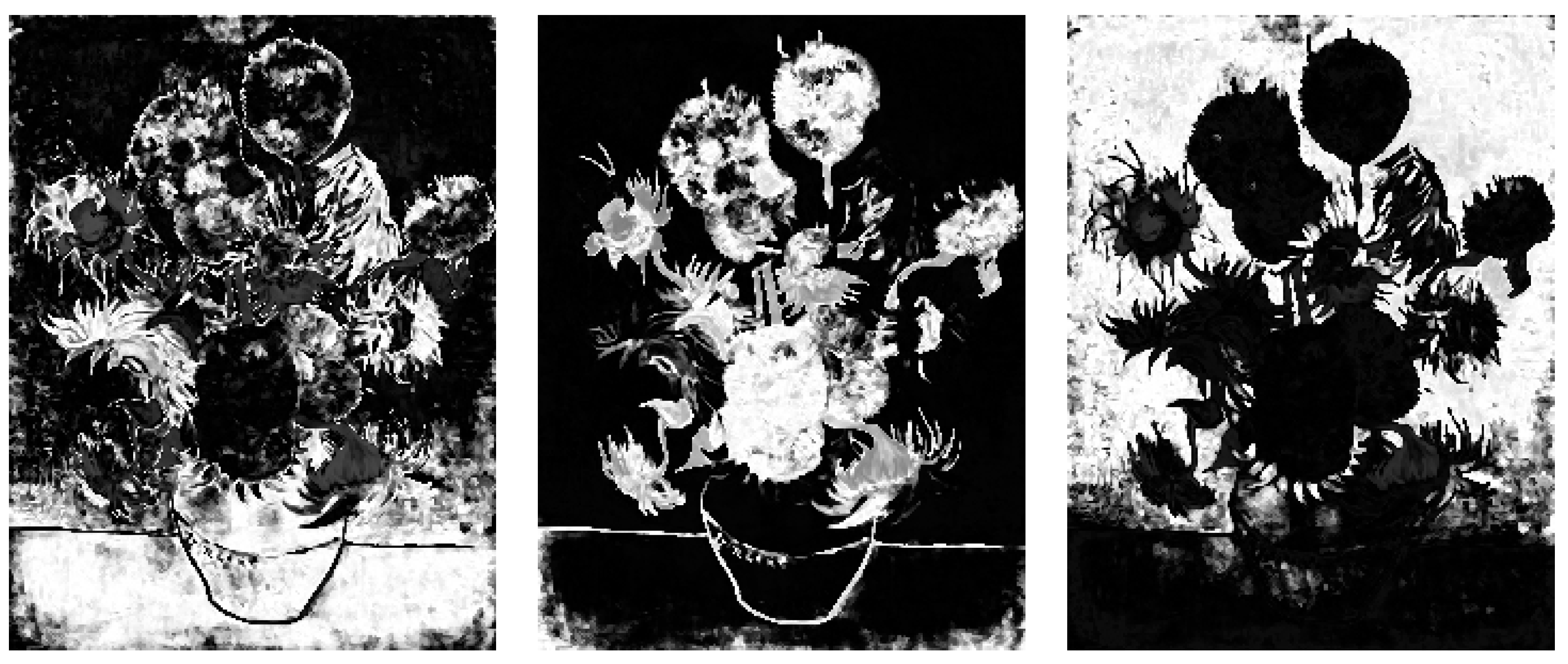
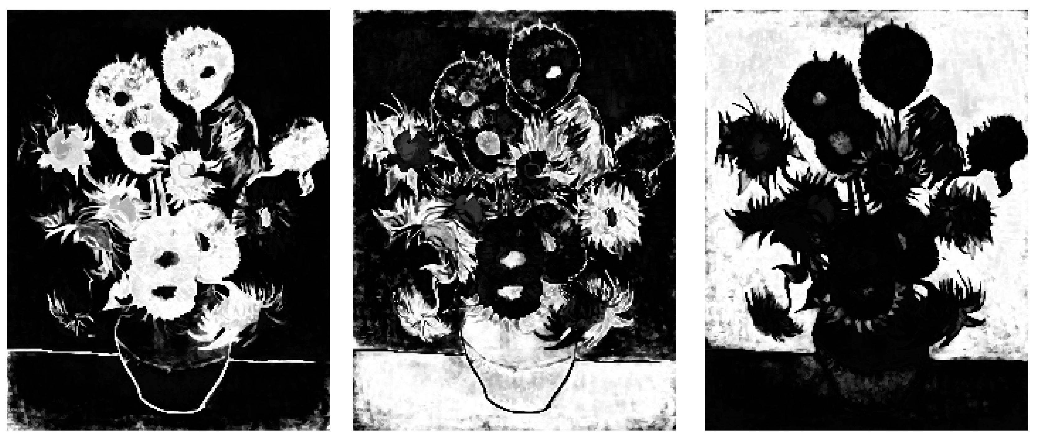
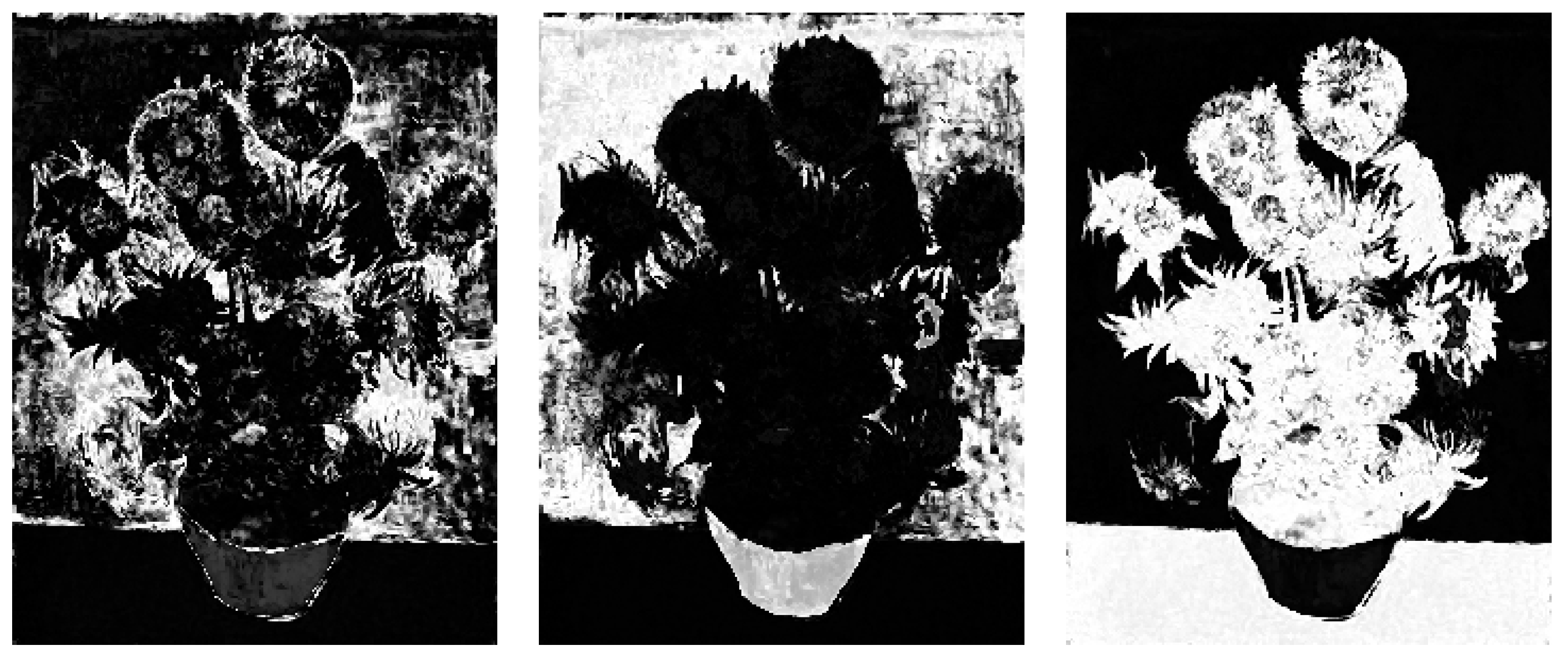
This image in each band is compressed using various compression rates and segmented setting the number of clusters (C) to 3. In
Figure 9,
Figure 10 and
Figure 11 shown the segmented images obtained using a compression rate = 0.25, respectively, in the R, G and B bands.
To measure the RMSE index of each segmented image with respect to the correspondent one obtained executing FCM on the source image, we decompress the segmented image via the bidimensional inverse F-transform.
In
Table 2 are shown the RMSE measures obtained in each band changing the compression rate.
The trend of the RMSE index in the three bands is shown in
Figure 12.
The results in
Figure 13 show that for compression rates greater or equal to 0.063 the value of the RMSE index is less than 3 in each band and the segmented images obtained executing FtbrFCM are comparable with the ones obtained executing FCM on the source images; conversely, for compression rates less than 0.063 the RMSE index rises rapidly and the loss of information due to compression becomes significant.
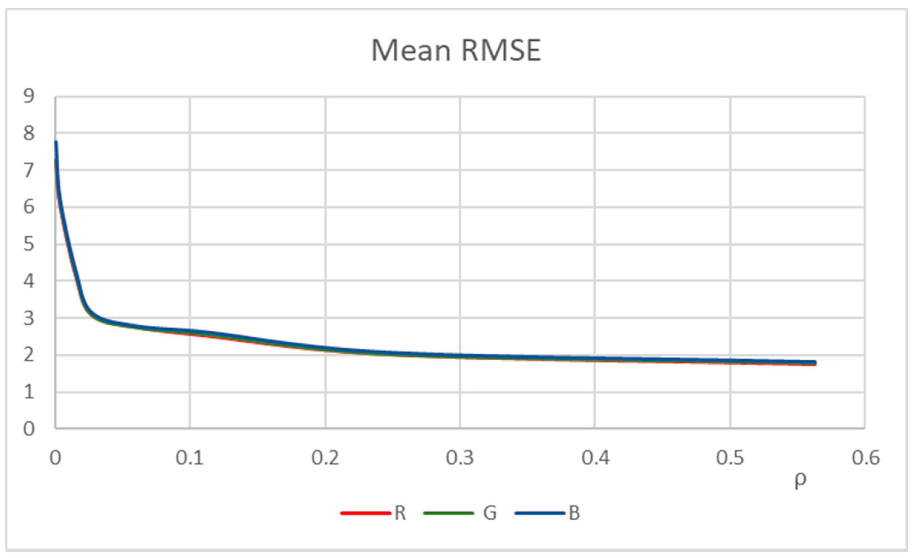
In
Figure 12 is shown the mean trend of the RMSE measured for all the images in the dataset in the three bands varying the compression rate.
For a compression rate ρ less than 0.11 the mean RMSE is greater than 3 and increases exponentially for higher compression. For compression rates greater than 0.11 the mean RMSE is less than 3 and the results obtained running FTbrFCM are comparable with the ones obtained running FCM on the source images.
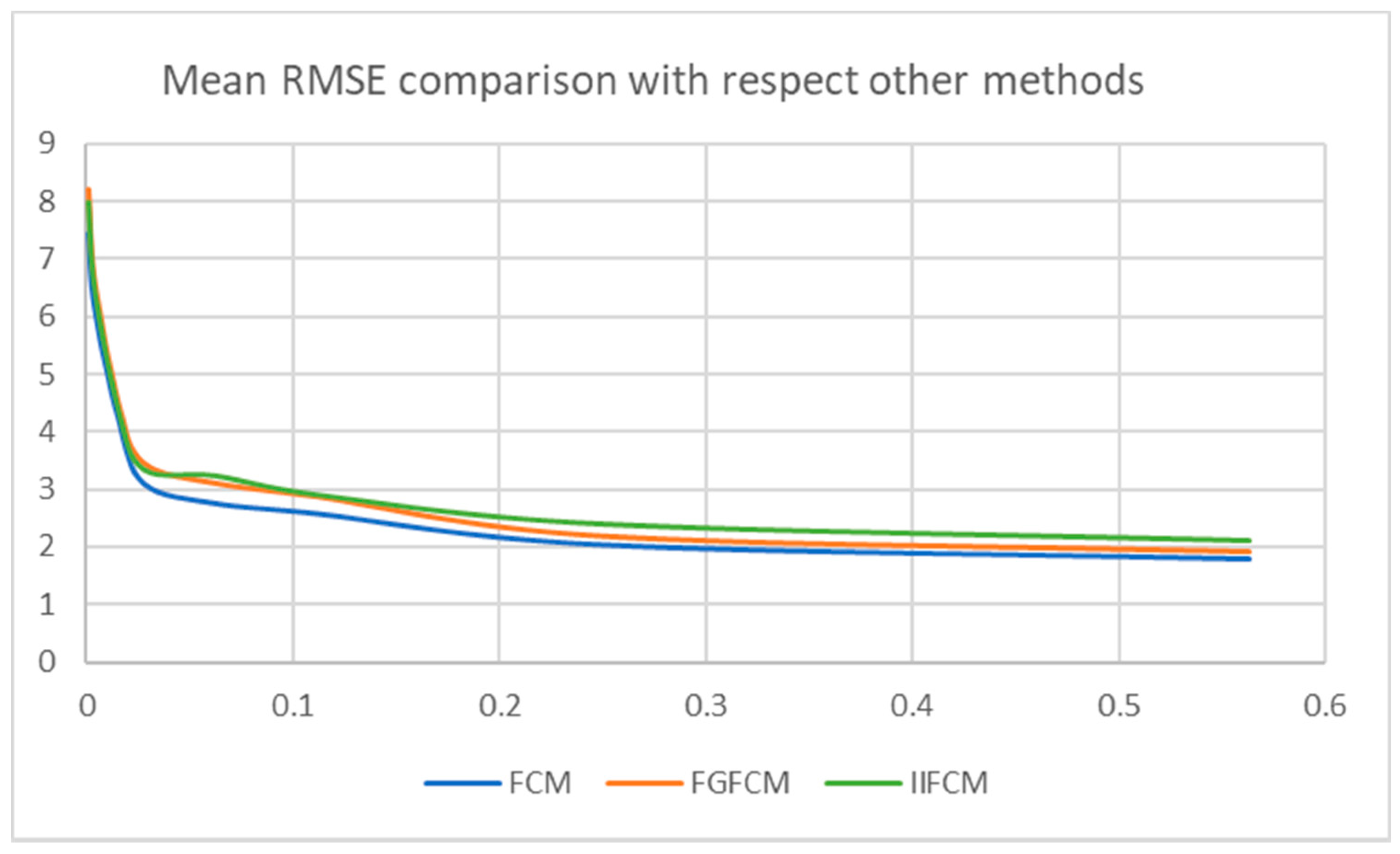
To compare the performances of FTbrFCM also with other image segmentation methods in literature we measure also the RMSE of FTbrFCM with respect to two fast FCM image segmentation variations called fuzzy generalized fuzzy c-means (for short FGFCM) [
16] and improved intuitionistic fuzzy c-means (for short IIFCM) [
17]; both these two FCM-based algorithms incorporate local spatial information considering spatial relations between near pixels and are more robust to noise than FCM improving its performances.
Figure 14 shows the trend of the mean RMSE calculated in any band varying the compression rate with respect to FCM, FGFCM and IIFCM.
Even if the average RMSE obtained with respect to FGFCM and IIFCM is greater than the average RMSE obtained with respect to FCM as the compression rate changes, the average RMSE obtained with respect to FGFCM and IIFCM remains below the threshold 3 for compression rates not lower than 0.1. These results show that for not substantial compression (ρ ≥ 0.1) the quality of the segmented images obtained executing FTbrFCM is also comparable with the ones obtained executing. FGFCM and IIFCM.
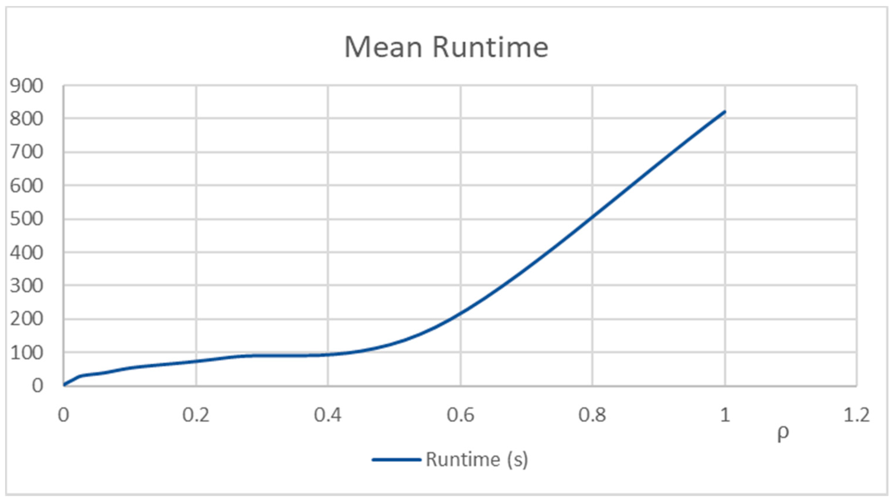
In
Figure 15 is shown the mean runtime in seconds, varying the compression rate. The run time measured where
ρ = 1 is the one obtained executing FCM on the source image.
Figure 15 show that for
ρ ≤ 0.25 the runtimes are less than 1/8 of the runtime of FCM applied on the source image. Since in our tests for all the images and in all bands using compression rates greater than
ρ = 0.11 the RMSE is less than 3, we deduce that using compression rates
ρ = 0.11 and
ρ = 0.25 all the segmented images are comparable with the ones obtained by executing FCM, and the runtimes are on average reduced to 1/8 with respect to the ones obtained executing FCM.


