Modeling Web Client and System Behavior

Abstract

Web systems are becoming more and more popular. An efficiently working network system is the basis for the functioning of every enterprise. Performance models are powerful tools for performance prediction. The creation of performance models requires significant effort. In the article, we want to present various performance models of customer and Web systems. In particular, we want to examine a system behaviour related to different flow routes of clients in the system. Therefore we propose Queueing Petri Nets, the new modeling methodology for dealing with performance issues of production systems. We follow the simulation-based approach. We consider 25 different models to check performance. Then we evaluate them based on the proposed metrics. The validation results show that the model is able to predict the performance with a relative error lower than 20%. Our evaluation shows that prepared models can reduce the effort of production system preparation. The resulting performance model can predict the system behaviour in a particular layer at the indicated load.

1. Introduction

Job scheduling, number of nodes, initial marking and many other parameters are the high importance in many computing systems, such as grid systems or cluster systems. Their performance is directly related to the efficiency of the Web computing systems. Some Web systems integrate and coordinate resources to intend the delivery of high-quality services.

Performance engineering could be used to make predictions about key performance metrics. We can detect some possible bottlenecks. Furthermore, we understand as-is performance and compare it with possible to-be performance. Various fields of engineering and science are using Performance engineering, as an important technology, to solve some problems that appeared in parallel systems like clusters (consists of nodes). In other words, performance engineering helps to answer questions [1]:

• How many nodes do we need to run handling different customer workloads?
• Which is the best client scheduling discipline?
• Are the system resources enough to serve clients’ requests?
• How long is a client waiting time?
• How much will clients’ waiting time reduce if more nodes would are deployed?

The most popular formal languages that could be used for modeling different Web systems include selected classes of Petri Nets and Queueing Nets. The main aim of this research is the development of the method to predict the customer performance of the Web system by using Queueing Petri Net (QPN) that models and simulates environment. We constructed a model for software components and hardware components. We prepared a simulation model to estimate customer response time. You can find in [2] validation of the developed method.

In this paper, we propose a method for analyzing the performance of Web systems. We use Queueing Petri Net Modeling Environment (QPME) software [3] to study parameters of systems widespread in Web systems. The main idea is to allow a hierarchical model specification to reduce the model size. This method is highly flexible and low-cost. Experimental results [2] show that this method could be applied to more complex Web systems. Quantitative analysis of QPNs is susceptible to the state space explosion problem because it is based on Markov chains. In Web system structures there are a lot of queues and tokens. Subsequently, the size of the state space of the underlying Markov chain grows exponentially. We used hierarchically combined Queueing Petri Nets to solve this problem [4].

The verification of Web system performance could not be based only on classical approaches like final tests. We need exclusively formal methods in the development process. That may significantly reduce costs and affect the product’s quality. This approach possesses two main parts. We build the QPN client and the system model with many parameters. Followingly, we implement this model using the QPME tool [3] and verify system performance. Earlier, we proposed a kind of potential application of this method to bigger structure consumer-to-business interactions [2,5].

1.1. Motivation

QPNs are a powerful and expressive performance modeling formalism. It has been shown, that even relatively small architecture models representing a Web system infrastructure may result in many different models. In this paper, we consider the client–server scenario in the Web system use case, where data is transferred from a large number of customers. The exponential growth in the number of clients naturally raises the question about the performance of the underlying system infrastructure. The performance evaluation of systems under dynamic load conditions poses new challenges. Scalability can be achieved at various levels. Choosing the right combination of parameters and technologies provides the flexibility needed to support a particular architectural choice.

The considered performance abstractions at the architecture level and analysis techniques serve as representative examples of typical solution techniques used in practice to predict performance. The case studies were chosen taking into account different modeling functions as well as different types of systems in terms of size and complexity. The purpose of our paper is to estimate the more accurate bottlenecks in traffic based on two classes of clients.

The target audience of this paper is performance engineers who want to apply resource demand estimation techniques to build a system performance model, as well as researchers working on improved estimation methods. The paper makes the following contribution:

• a review of the most modern methods for estimating the performance of an Internet system,
• a classification scheme of approaches to estimating resource requirements,
• an experimental comparison of a subset of the estimation approaches.

1.2. Organization

The rest of this paper is as follows. Section 2 includes related works. Section 3 analyzes an overview of Web system structures. Section 4 describes several modeling approaches. Section 5 introduces some client and system models. Section 6 presents the simulation results. Finally, Section 7 concludes the paper and indicates possible directions for future work. (We assumed that the reader knows QPN formalism. QPN model of Web system was defined in [4]).

2. Related Works

Computer and communication networks development, manufacturing systems assessment and business processes analyses mainly affect performance evaluation. In the past few years, most of the works have been focusing on Web systems, which are very efficient and able to handle numerous incoming requests. There are two mathematical formalisms to solve problems of performance evaluation and analysis: Queueing Nets and Petri Nets. We find the queueing method as a well-known one and common in dealing with limited resources. Queueing Net makes it possible to calculate the throughput of the subsequent elements of a computing process represented as a network of queueing systems. Petri Net is a specific graph where the token flow through the network. It could be interpreted as the reallocation of the load in the evaluated system [6].

2.1. Works Based on Various Formalisms

Existing modeling approaches divide according to various criteria. We can find the related works grouped into publications based on stochastic models such as Queueing Net (classical product-form, extended or layered) and stochastic models such as Petri Nets. In the first group, there are some opened and closed queueing models. In [7] the author presents the model application of server cluster and database server. In the paper, [8] authors propose the model software systems using classical queuing theory and statistical response time models in parallel. This approach allows users to tailor the model for each analysis run, based on the performed adaptations and the requested performance metrics. In [9] the author prepared the multi-tiered application model by using Mean Value Analysis (MVA) and compared performance with real performance values. Recent publications [2,10] use QPN for performance modeling of Web structure and compare with the production system performance. To manage the routing of packages in Web structures, we can apply elements of the control theory. In turn, in the second group, there are different variants of the Petri Nets [10,11]. In [12] for some modes of emergency actions, Petri Nets models are proposed. The Apache Storm model was presented in [13]. The author used Generalized Stochastic Petri Nets for performance checking. Proposed in [14] techniques of analysis could help in the context of Web systems performance, that nowadays confront the era of Big Data. Various papers propose the arrival of stream modeling and its analysis. According to the Web system modeling method introduced in [10] the modeled system (Platform as a Service designed to host Web applications) retains a structure similar to an open queueing system. Analysis of the distribution of data packages within the system makes it possible to find out some potential bottlenecks [6]. To efficiently carry out the randomly arriving data [15], the number of overlapping (concurrent) request/response sessions utilized by the sending node, is higher than in typical client–server communications.

Furthermore, there are some mathematical models for predicting the performance of the Web system. Almost in all cases, the authors conducted experiments [5,16]. This is the second way for performance engineering. The use of simulations models and experiments allows verifying the proposed models. Moreover, it greatly influences the validity of the systems’ development. In the article [17] they examined request distribution strategies used in one-layer and two-layer architectures of Web systems. In paper [18] they discuss current software architectural styles, patterns, and development platforms based on client-side and server-side technologies. Some authors in [19] use Production Trees, the new modeling methodology for dealing with availability issues of production systems.

2.2. Previous Works Based on Queueing Net, Time Colored Petri Net and QPN Formalisms

Performance models are an abstraction of a combined hardware and software system describing its performance of relevant structure and behaviour. My models’ evolution: Queueing Net (Queueing Networks are not good at expressing or modeling concurrent events (e.g., fork and join situations, blocking, etc).) (based on mean value analysis as Queueing Theory technique and QNAT tool), Time Colored Petri Net (Petri Nets are good for representing concurrency but do not lend themselves to performance analysis. Adding time to Petri Nets enable them to be used in modeling.) (based on Time Colored Petri Nets formalism and Design/CPN tool) [5] and QPN (based on Queueing Petri Nets formalism and QPME tool) [2]. These formalisms are highly popular and beneficial for qualitative and quantitative analysis [7].

2.3. Current Work Based on QPN Formalism

Mathematical formalism successfully merging Queueing Net and Petri Net is called Queueing Petri Nets (QPNs). Among other applications, QPN [3,7,20] successfully applied the distribution of Web systems modeling and performance evaluation [2,10]. The formalism is widely used in other areas, e.g., authors show [21] how the language of sequence diagrams is mapped onto an equivalent language of QPNs through formal transformation rules. The article [22] covers database performance in QPN formal models. The author presented and classified some fundamentals of the queueing system theory and queueing system models. This paper presents a systematic survey of the existing database system performance evaluation models based on the queueing theory. The workload of the Web system under the study describes it quantitatively and qualitatively. Besides, quantitatively performance modeling, QPN could also take into consideration hierarchical structures. It describes the dependency relationship among layers in multilayered systems. QPN models services with ease for Web systems.

Previously [2,10], the impact of one query class was examined for the others. The error for one client class is between 4.68–29.36% [4]. Experiments [5] demonstrated that too much fragmentation of requests classes does not make sense because only two request classes have the greatest influence: sell/buy and portfolio. To simplify the model, the previous simulations concerned one class. The content of this work will be using (routing) different resource through request classes. The workload intensity of a system is characterized by the number of requests of each class executing concurrently. It is called the customer population [23]. All systems have different response time requirements for different clients [24]. The modeling approach presented in this paper differs from that of previous work because we model more types of requests. We add division into classes of queries to the QPN model and we use hardware and software elements by individual classes. As indicated by the experiments [5] the different types/classes of clients associate with different behaviours: different periods for query arrivals, demand services or network routing.

The web system must be analyzed in terms of both quality and quantity. Queueing Nets are suitable for modeling hardware competition by using queues and scheduling disciplines. Petri Nets are appropriate for blocking and synchronizing modeling due to the use of tokens representing tasks. QPN has the advantages of Queueing Net (e.g., evaluation of the system performance, the network efficiency) and Petri Net (e.g., logical assessment of the system correctness). QPN allows a wide range of Internet system research. QPN formalism integrates hardware and software elements into one model. Due to these properties, QPN holds greater expression than Queueing Net (quantitative analysis) and Petri Net (qualitative analysis).

According to other works, we selected parameters that have the greatest impact on performance. In this paper, we study parameters of systems and propose the QPN method for analyzing their performance, which can be easily implemented in Queueing Petri Net Modeling Environment software by potential system architects. The construction of the real system was the subject of earlier works. Simplified models were also included there. The most important achievement of the proposed model is the improvement of the simulation result for two classes of clients about the results for one class of clients. The results are closer to the results achieved in the experiments of the real cluster system. Two query classes completely change the flow of tokens in the model. The results of experiments in the real environment include even more classes, but as indicated in the article only two of them have a significant impact on the system performance.

This approach could be treated as an extension of the papers [2,10], where we proposed and validated the QPN models for the Internet system. Additionally, in the previous article [5], we also proposed QPN models for one kind of the Web system with one class of customers’ requests. Presently, the model with many classes (in this case two) is used, adapting it even more to reality. In most cases, the models consist of one class of clients. In those models, scientists do not distinguish between different behaviours and flows of web system clients. Models prepared for this article possess more parameters, therefore, there are more detailed.

The final results of the simulations include the average number of tokens in the queueing system, location or depository, the average probability of the token in the queueing system, place or depository, the average bandwidth of the queueing system, place or depository and average time spent in the place [5].

3. Web System Architecture

3.1. Clustering

Nowadays, an increasing number of companies depend on the business processes running on their servers. International companies operate with clients all over the world, accessing their services at any time. Web systems are usually used to describe computing that spans multiple machines. A cluster is two or more computers (nodes) that work parallel together to perform tasks. There are two main reasons for clustering. First one is to provide fail-over capability and increase the availability of systems. High availability clusters are implemented primarily to improve the robustness of services which the cluster provides. The second one is to provide parallel calculating power and improved system performance.

There are four major types of clusters:

• High Availability also known as Fail-over Clusters,
• Load Balancing,
• High Performance.

High Availability (HA) is becoming a requirement for an ever-increasing number of business Web applications. Clustering emerges as a natural solution for delivering high availability for a significant number of clients. Load Balancing (LB) is useful to distribute client requests to several nodes. Performance means system throughput under a given workload for a specific time-frame. High Performance (HP) clusters use cluster nodes to perform concurrent calculations. Clustering is a method of grouping two or more nodes with the goal of increasing the availability and performance of such a group, compared to a single server.

3.2. Nodes in Cluster-Based Web Architecture

A multi-tiered or multi-layered architecture is a type of architecture composed of tiers and layers. This is the traditional method for designing self-independent software and hardware structures. The use of a layered approach (modular user interface, business logic, and data storage layers) is good for the system design (e.g., scalability, performance, and availability). These architectures provide many benefits in production environments.

Building a highly available and scalable system that performs well is certainly not a trivial task. The term performance of the Web system encompasses several meanings. By separating layers we could scale each of them independently. By having separated layers we can also increase performance. The Web system layers compose of many servers/nodes. Layers are dedicated to proper tasks. Moreover, they exchange customer requests with each other. Servers and services are used to receive requests submitted by clients.

Web system logical architecture is constructed of layers [2]. The following four are the most common: a presentation layer (a presentation tier in a multi-tiered architecture), an application layer (a service layer for client requests), a business layer (a domain layer for the control of the transactions) and a data access layer (a persistence layer with a data storage system). In our approach [2] presented architecture has simplified into two layers: Front-End (FE) and Back-End (BE). The clustering mechanism is used in both layers. These simplifications exert no influence on the modeling process, which has illustrated in [2,7].

3.3. Distributed Computing

Distributed computing is a field of computer science studying distributed systems. Distributed system consists of multiple nodes that communicate via the network. The computers in each node interact with each other to accomplish a shared goal. In this approach, the cluster is created from a number of computers to work together as a team. These parallel systems, installed with a large number of CPUs, provide good results for both real-time and near-real-time applications using data streams.

Analytics and data mining are often performed using parallel approaches on Web systems. The challenge is finding a way to transform raw data into valuable information. To capture value from those kinds of data, it is necessary to upgrade technologies and techniques that will help individuals and organizations to integrate, analyze and visualize different types of data. Distributed Web systems along with management and parallel processing principle allow analyzing Big Data. Different aspects of the distributed computing paradigm resolve different types of challenges involved in the analytics of Big Data. A lot of what is called Big Data does not involve all that much data. It is more about how the data is analyzed rather than the simple quantity of data.

3.4. Different Customers

All of the machines on the Internet are either servers or clients. In addition, the machines that provide services to other machines are servers. The machines that are used to connect to those services are clients. Clients that come to a server machine do so with a specific intention, therefore, clients direct their requests to a specific software server running on the server. For example, if you are running a Web browser on your PC, it will want to talk to the Web server on the server machine. Client/server architecture is what makes the Internet possible. The client is a computer hardware device or software that accesses a service made available by a Web system.

To understand customer behaviour along with the better allocation of resources for different Web clients and to generate the highest profit, it is necessary to be able to identify and segment different types of Web customers. By better understanding of the different types of customers, businesses could be better equipped to develop successful Web system architectures. Low customer service time experience translates into higher customer satisfaction.

Although behavioural patterns are unique and individual to every person, there are certain similarities in those patterns. It should be considered as taking a different approach to each group of consumers, because different customers have different personalities, and hence expectations and needs. The better adjustments to each group you will make, the higher customer satisfaction will be. We checked client behaviour in the real system [5] on IBM DayTrader benchmark.

Web clients divide into certain groups as for performed tasks, time spent in IS and generated load. There are types of clients for performed tasks. A classic client uses the basic properties of the system (logging into the system, browsing through the offer of the service, using the service, transactions, determining the balance of their account, checking the correctness of the transaction). “Guest” client looks only through information on the whole problem (checking the possibilities of the system, accidental opening of a web site as a result of surfing the Internet). An administrator is a person managing the net (logging into the system with administrator’s rights, introducing necessary changes, the configuration of system operation and its specific behaviour). The second type of clients relates to the time they spend in the system. There are sporadic (short-term) clients downloading needed information or surfing through web sites and by contrast, there are permanent (long-term) clients using some of the functions offered by the system. The third type of clients connects to the loading of the system. They are divided into surface clients who do not use the whole but only the first layer and opposite to the standard clients who use the inner layers. Additionally, some partial clients use different parts of the system.

4. Queueing Nets and Petri Nets Models

In our solution, we propose QPN models predicting the performance. One of the basic performance engineering parameters, which is response time, was chosen for verification of the performance.

QPN models have been developing for different input parameters as well as different clients and the system’s parameters. Prepared parameters and architectures in the form of models enable the description of hardware and software to map. This realistically allows imitating system behaviour.

4.1. Queueing Nets and Petri Nets in the Same Model

Queueing Net (quantitative analysis, e.g., evaluation of logical system correctness) has a queue. In the case of arriving some customer requests could not receive immediate service due to busy servers, the queue is formed. Client requests enter the queue and must wait until a processor is idle. After waiting time the processor services the client request with predefined scheduling strategy. Queue systems represent system components and they are connected to one network. The main parameters of the queue system are:

• Arrival process is a mathematical model for the time between request arrivals to the system e.g.,: Poisson, Erlang, hyper-exponential, general. (We analyzed queueing systems without external clients arrival.)
• Service time is defined as the time required to serve a customer request e.g.,: logarithmic, chi-square, hyper-exponential, exponential. Service times are Independent and Identically Distributed (IID). (We analyzed queueing systems with the exponential clients’ service time.)
• Scheduling strategies define the strategies used to allocate the processor e.g.,: First In First Out (FIFO), Last In First Out (LIFO), Last In First Out with Preempt and Resume (LIFO-PR), Round Robin (RR) with a fixed quantum, Small Quantum ⇒ Processor Sharing (PS), Infinite Server (IS) = fixed delay, Shortest Processing Time first (SPT). (We used IS for clients machine, PS for FE nodes and FIFO for BE nodes.)
• Number of processors. (This paper considers a single server queue.)
• Number of buffers is waiting room size. (Size of the queue is infinite.)

Petri Net (qualitative analysis, e.g., assessment of system performance, network efficiency) has tokens representing requests. Petri Net describes dynamics based on rules of tokens flow. Main parameters are:

• set of places,
• set of transactions,
• initial marking (number of tokens),
• incidence function (routing probability),
• token color function.

QPN adds queue and time aspects to model [4].

4.2. Theoretical Introduction

At the beginning, performance goals are defined. Performance engineering objectives are: performance prediction, performance analysis and bottleneck analysis. Performance engineering methodology scenario is:

• understanding the operation of the system,
• determine the system load,
• measure system parameters,
• build a performance model,
• model verification and validation,
• load changes,
• predicting system performance,
• analysis of various scenarios.

This approach was used to evaluate the performance of a Web system to support decision concerning scaling resources for the Web structure. Performance metrics are e.g., throughput or response time. The laboratory environment was used for experiments (for checking input parameters and validation [5]). Followingly, the performance model was built for simulations [10] (for checking the response time parameter). Parameters that determine the client response time are following:

• number of clients, workload intensity (think time (The think time adds delay in between successive requests to the system from populated concurrent clients.), different types of arriving requests of clients are different behaviours) for the client.
• number of hardware elements (nodes in FE and BE layer), hardware connections (routing), software parameters (service resources as threads and connection pools), scheduling strategy, service demand (Service demand in milliseconds $\left[ms\right]$ is the time needed to serve one request at the station.) for the selected class in a specific resource (1), excluding the waiting time for a resource (it does not depend on the load) for the system.

$$\begin{array}{c}Avg.ServiceDemand\left[ms\right]=\\ Avg.Utilization/Avg.RequestThroughput\left[RPS\right]\end{array}$$

(1)

We could divide our modeling method into five steps (in this article we present steps from 2 to 5). At the beginning there is the measurement of system’s parameters [2,5] (first step). The second one is to model a Web system abstractly (including client model) (second step). Subsequently, we refine the abstract model into a more detailed model (third step). Finally, we propose how to analyze performance-models of request classes are chosen (Figure 1) (fourth step). Validation is performed on the example of real infrastructure and real Web system [4] (Service demand for two client-classes (system).) (fifth step).

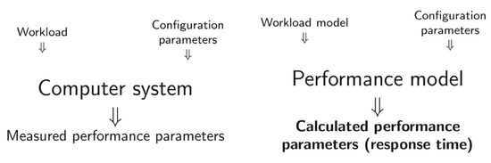
Figure 1. A diagram of the response time measurement process (difference between real computer system and performance model).

In [4] we specified the model parameters for formal analysis of the Web system. In the same paper, we proposed the fundamental equation more applicable to our performance engineering.

4.3. Client Model

Model of a i client type has been marked as $M{K}_i$. Model of a particular type of client depends on numerous parameters, such as sort of services, time limits imposed on collective time of service execution, intensity and distribution of clients’ localization. Therefore i client type model can be defined as the following Equation (2).

$${\left(M{K}_i\right)}_k={(O_i,D_i,F_i)}_k$$

(2)

where:

• $O_i$—client service type,
• $D_i$—time limit, i.e., time interval in which the client has to be serviced,
• $F_i$—function describing arrivals of a particular type of clients.

It has been assumed that every Web client could be attributed to a certain client class. Defining a set of client types (classes) as $TK$ in addition to assumption that the client types number is k, we obtain Equation (3).

$$T{K}_k=\{{\left(M{K}_1\right)}_k,{\left(M{K}_2\right)}_k,\dots {\left(M{K}_i\right)}_k\}$$

(3)

Depending on a client type we can determine different kinds of servicing Equation (4).

$$O_i=\{{\left(O_{WS}\right)}_i,{\left(O_{AS}\right)}_i,{\left(O_{DB}\right)}_i\}$$

(4)

where:

• $O_{WS}$—servicing on a Www Server,
• $O_{AS}$—servicing on an Application Server,
• $O_{DB}$—servicing on a Database Server.

Time can be calculated for each type of servicing (Equation (5)).

$$C{\left(O_{all}\right)}_i=C{\left(O_{WS}\right)}_i+C{\left(O_{AS}\right)}_i+C{\left(O_{DB}\right)}_i$$

(5)

where:

• $C{\left(O_{all}\right)}_i$—total time of servicing for clients of $M{K}_i$ type,
• $C{\left(O_{WS}\right)}_i$—time of servicing for client of $M{K}_i$ type on a www server,
• $C{\left(O_{AS}\right)}_i$—time of servicing for clients of $M{K}_i$ type on an application server,
• $C{\left(O_{DB}\right)}_i$—time of servicing for clients of $M{K}_i$ type on a database server.

The total servicing time must be lower than the imposed time limit (time out) Equation (6).

$$C{\left(O_{all}\right)}_i<D_i$$

(6)

Completing this condition does not mean completing time limits for a particular type client.

Individual servicing times must meet the following dependencies Equations (7) and (8).

$$C{\left(O_{WS}\right)}_i<D{\left(O_{WS}\right)}_i$$

(7)

$$C{\left(O_{AS}\right)}_i+C{\left(O_{DB}\right)}_i<D{\left(O_{AS+DB}\right)}_i$$

(8)

Whereas individual time limits must meet the following conditions Equations (9) and (10).

$$D{\left(O_{WS}\right)}_i\le D_i$$

(9)

$$D{\left(O_{AS+DB}\right)}_i\le D_i$$

(10)

For instance, if a time limit $D_i=5$ time units, and individual $D{\left(O_{WS}\right)}_i=4$ and $D{\left(O_{AS+DB}\right)}_i=3$, then the above dependencies are not met.

A function that modeling the arrival of a particular type of clients’ queries depends on the client type and could be described through Equation (11).

$$F_i=(f_i,{\lambda }_i,p_i)$$

(11)

where:

• $f_i$—distribution of probability of clients’ arrivals (degenerate/determined (A determined distribution means that the times are constant and there is no variance.), Poisson, etc.),
• ${\lambda }_i$—average intensity of arrivals,
• $p_i$—another parameter of distribution (if it exist).

In many uses, Web client must be served in the allotted time. Checking if Web client meets the time limits, could be carried out in certain cases with the application of time analysis. The most typical distributions analyzed within the theory of mass service are degenerate/determined distribution, Poisson distribution. For the determined distribution, the process of request arrivals is precisely determined, and the time intervals between consecutive arrivals $T_i$ are constant Equation (12).

$$\sum _{i=1}^n\frac{C_i}{T_i}$$

(12)

where:

• $C_i$—time of task execution,
• $T_i$—period of task occurrence,
• $T_i=D_i$,
• $D_i$—time limits of the task.

For exponential Poisson distribution the probability of k arrivals in any interval of t length is Equation (13).

$$p_{\lambda }(x=k)=\frac{{\left(\lambda t\right)}^k}{k!}{e}^{-\left(\lambda t\right)}$$

(13)

for $k=0,1,2,\dots$

where:

• x—random variable (amount of tasks in t time),
• $\lambda$—intensity of task arrivals.

Average arrival intensity ${\lambda }_i=1/T_i$, where $T_i$ is an interval between consecutive arrivals. System clients (tasks) appear by Poisson distribution and the time of awaiting them is exponential distribution (continuous).

We investigate two typical Web clients. The first one only browses through Web sites (superficial), therefore it is not a client using the whole of the system (FE and BE layer), but only its first layer (FE). The second one-the actual client utilizes most of the functions provided by the whole system Equation (14).

$$\begin{array}{c}T{K}_3=\{{\left(M{K}_1\right)}_3,{\left(M{K}_2\right)}_3,{\left(M{K}_3\right)}_3\}\end{array}$$

(14)

$M{K}_1$—a model for a client only browsing through FE layer of the system Equation (15).

$$\begin{array}{c}\begin{array}{c}M{K}_1=(O_1,D_1,F_1)\hfill \\ O_1=O_{WS}\hfill \\ C{\left(O_1\right)}_1=C{\left(O_{WS}\right)}_1\hfill \\ C{\left(O_{WS}\right)}_1<D{\left(O_{WS}\right)}_1\hfill \\ D{\left(O_{WS}\right)}_1\le D_1\hfill \\ F_1=(f_1,{\lambda }_1)\hfill \end{array}\end{array}$$

(15)

$f_1$—Poisson distribution.

$M{K}_2$—a model for a client browsing all system layers Equation (16).

$$\begin{array}{c}\begin{array}{c}M{K}_2=(O_2,D_2,F_2)\hfill \\ O_2=(O_{WS},O_{AS},O_{DB})\hfill \\ C{\left(O_2\right)}_2=C{\left(O_{WS}\right)}_2+C{\left(O_{AS}\right)}_2+C{\left(O_{DB}\right)}_2\hfill \\ C{\left(O_{WS}\right)}_2<D{\left(O_{WS}\right)}_2,C{\left(O_{AS}\right)}_2+C{\left(O_{DB}\right)}_2<D{\left(O_{AS+DB}\right)}_2\hfill \\ D{\left(O_{WS}\right)}_2\le D_2,D{\left(O_{AS+DB}\right)}_2\le D_2\hfill \\ F_2=(f_2,{\lambda }_2)\hfill \end{array}\end{array}$$

(16)

$f_2$—Poisson or determined distribution.

The third client could be the system administrator. It is a client who is similar to the second type of client presented earlier, with the difference that this user uses another part of the system. Its servicing does not require meeting strict time limits. Its behaviour in the system could be easily predicted and defined because it is not a strange user, who could be unforeseeable. Nevertheless, its actions should have the highest priority due to the necessity of performing certain administration tasks Equation (17).

$$\begin{array}{c}\begin{array}{c}M{K}_3=(O_3,D_3,F_3)\hfill \\ O_3=(O_{WS},O_{AS},O_{DB})\hfill \\ C{\left(O_3\right)}_3=C{\left(O_{WS}\right)}_3+C{\left(O_{AS}\right)}_3+C{\left(O_{DB}\right)}_3\hfill \\ C{\left(O_{WS}\right)}_3<D{\left(O_{WS}\right)}_3,C{\left(O_{AS}\right)}_3+C{\left(O_{DB}\right)}_3<D{\left(O_{AS+DB}\right)}_3\hfill \\ D{\left(O_{WS}\right)}_3\le D_3,D{\left(O_{AS+DB}\right)}_3\le D_3\hfill \\ F_3=(f_3,{\lambda }_3)\hfill \end{array}\end{array}$$

(17)

$f_3$—Poisson or determined distribution.

With simplified assumptions stating that the time of task arrival distribution is determined, it is possible to check if the time limit condition met for all of the tasks. In this article, we use simplification $WS=FE$ and $AS+DB=BE$.

5. System Model

The discrete-event simulation methods are employed to analyze the constructed models. Based on previous works [4,10] we used two-layered Web system as an example of a system with clusters in both layers and with selected groups of clients (classes).

QP Net

Performance modeling and prediction tools are required to generate accurate outputs with minimal input sample points. An important tool used in this part of our research was original QPME simulator consists of SimQPN (discrete event simulation engine), Queueing Petri Editor (Net Editor, Color Editor, Queues Editor). The simulator was designed to enable integration between formalism-based simulation and software/hardware aspects. QPME is an open-source tool for stochastic modeling and analysis based on the QPN modeling formalism. We implemented executable models in QPME tool. QPN net (Figure 2) is used to predict customer response time. The arrival process, waiting room, service process, and additionally depository describe each queueing place on sub-page $Sub-FE$ and $Sub-BE$. We adopted several queueing systems most frequently used to represent the properties of the Web system components. Resources such as queueing places in the system under simulation may be hardware elements (CPU and disk I/O) and resources such as places may be software elements (threads and connection pools).

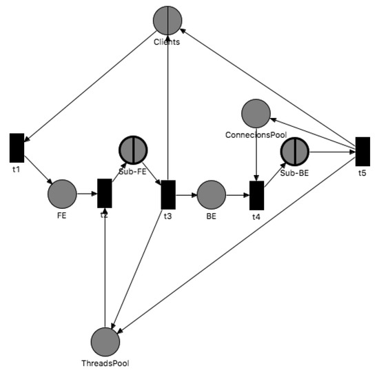
Figure 2. Main page of Web system model [4].

$FE\_CPU$ and $BE\_I/O$ queueing places model nodes in FE and BE layer respectively. $FE$ and $BE$ places are used to stop incoming requests when they have been waiting for application server threads and to stop incoming requests when they have been awaiting database server connections. $ThreadsPool$ place and $ConnectionsPool$ model application server threads (application server machine) and database server processes (database server machine) respectively. Customer requests are in closed network (Figure 2). Requests are sent to the FE layer and placed in $FE$ queueing places to get service. After service in FE, layer requests could be forwarded to the BE layer to get service. The BE layer is responsible for data handling. After service in the BE layer, the customer requests could be forwarded to the client. Every layer in different cases is presented on the figure (Figure 3).

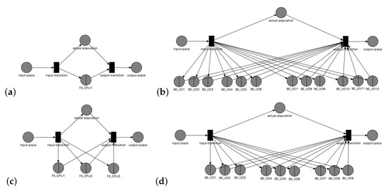
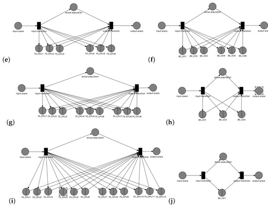
Figure 3. Sub-FE and Sub-BE pages modeling overview: (a) $FE1$, (b) $BE12$, (c) $FE3$, (d) $BE9$, (e) $FE6$, (f) $BE6$, (g) $FE9$, (h) $BE3$, (i) $FE12$, (j) $BE1$.

We have four types of tokens (Every token that could be resided in a place has a type (color).) (Figure 4a): client-classes ($k1=x1$ and $k2=x2$), application server threads and database server connections.

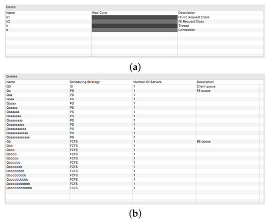
Figure 4. QPME tool configuration: (a) token colors, (b) example queues.

One server (Figure 4b) utilizes queueing systems. Clients machine is modeled by queueing place with IS scheduling strategy (-/M/1/PS/∞ queueing system). Nodes of the FE layer are modeled by queueing places with PS scheduling strategy (-/M/1/PS/∞ queueing systems). Nodes of the BE layer are modeled by queueing place with FIFO scheduling strategy (-/M/1/FIFO/∞ queueing system).

At present we possess an executable QPN model in the simulation sense. An increasing number of parameters (for particular client type: number of clients, flow probability, service demand on a particular element, service distribution probabilities on a particular element, number of nodes in FE and BE layer) is subject to modeling in our models. The models presented in the literature are limited to a few basic parameters and simple architecture of the system. The structures presented in figure (Figure 2) and (Figure 3) are similar to previous models but parameterization of these models is quite different.

6. Simulations with Different Parameters

In this section, there will be presented the simulation results of models with a different number of nodes in the FE and BE layer, different client and system input parameters. We investigate the customer request response time.

The performance problem was evident in the first layer (FE). After adding the FE nodes, the response time decreased (Figure 5). The subsequent addition of FE nodes in the FE layer increased the response time. The number of tokens in $Clients$ place means the number of clients. This value of workload intensively increased. We adopted different scenarios in which there were two request classes. As a result of an increased number of FE and BE nodes, the response time of client requests improved. When the number of nodes increased, simultaneously a whole number of threads in the FE layer and connections in the BE layer also increased. As we can see (Figure 5 ($p1$ and $p2$ think time for different request classes. Number of clients: $x_1=250,x_2=250$.)) overall customer response time decreased while the number of nodes was increasing (for 15 [RPS]). A difference in response time between 1st and 3rd nodes was relatively small. For one FE node architecture, response time for all cases was the biggest. Overall system response time increased with increasing workload, even with a larger number of nodes.

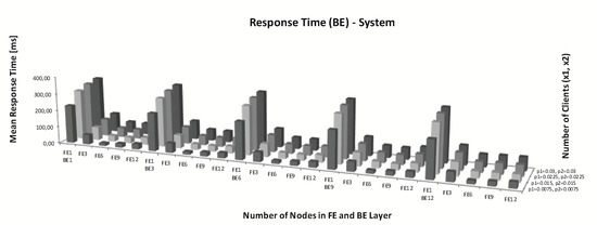
Figure 5. Response time for different number of nodes in Back-End (BE) and Front-End (FE) layer.

Table 1 presents results of the analysis between simulation for one class of clients, simulation for two classes and real system experiments. The calculated simulation error was, therefore, smaller for two client-classes, which meant that the distribution of requests in the model was closer to reality. The system with many client-classes was used for experiments. As evidenced in [2], only two of them were significant, therefore, the results of experiments were used for comparison. The calculated simulation error was smaller for two client-classes, which means that the distribution of requests in the model was closer to reality. The error for two client classes was between 9.25–13.65% [4] and it was smaller than for one class for the same input parameters.

Table 1. Response time error for one and two classes (FE3 and BE1).

Client Think	Two Classes of	One Class of	Measured	Error for One	Error for Two
Time [ms]	Clients [ms]	Clients [ms] [4]	[ms] [2]	Class of Clients [%]	Class of Clients [%]
66.66	76.46	56.23	65.12	17.41	13.65
33.33	110.32	76.78	85.28	29.36	9.96
22.22	121.23	99.38	110.83	9.38	10.34
16.67	126.59	109.76	120.94	4.68	9.25

Simulation with Changed Parameters

Increasing the number of clients (new case: $x_1=2500,x_2=250$) worsens the problem in FE-increasing the number of clients causes waiting for FE resources (Figure 6). The only expansion of FE nodes to 12 gives a comparable response time with a smaller load. For example $x_1=2500$ clients and 30 [RPS] gives 75,000 [RPS] (total for one class). In the case, $BE3$, $BE6$, $BE9$, and $BE12$ is the same situation.

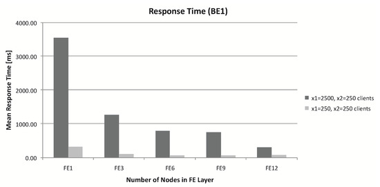
Figure 6. Response time for $x1=2500$ clients (BE1).

With the same number of clients, increasing the number of threads (3000) in $FE$ place reduces the waiting time for resources in the FE already for $FE1$ (Figure 7).

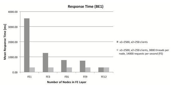
Figure 7. Response time for $x1=2500$ clients (BE1), 3000 threads per node in FE layer.

Next cases (Figure 8):

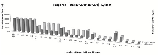
Figure 8. Response time for $x1=2500$ clients, 3000 threads per FE node, 4000 process per BE node.

• $x1=2500$ clients and 30 [RPS] gives 75,000 requests, 3000 threads per node and 14000 [RPS] for FE ($x1$ and $x2$) and 40 processes for each database node (Table 2),
  Table 2. Case with parameters: 3000 threads per FE node, 40 database connections per BE node.

  		Sub-FE.FE_CPU	Sub-FE.FE_CPU	BE	Sub-BE.BE_IO	Sub-BE.BE_IO
  		(qplace:queue)	(qplace:depository)	(place)	(qplace:queue)	(qplace:depository)
  BE1	FE1	5.12	0.00	290.58	5.35	0.00
  BE1	FE3	0.28	0.23	294.46	5.34	0.00
  BE1	FE6	0.47	0.69	293.76	5.33	0.00
  BE1	FE9	0.68	1.26	294.25	5.34	0.00
  BE1	FE12	0.89	1.90	294.06	5.34	0.00
  2.5 BE3	FE1	162.69	0.00	0.00	0.67	0.35
  BE3	FE3	0.49	0.39	82.27	3.47	2.05
  BE3	FE6	0.50	0.74	82.14	3.48	2.03
  BE3	FE9	0.69	1.14	82.25	3.47	2.05
  BE3	FE12	0.90	1.91	82.20	3.48	2.04
  BE6	FE1	162.41	0.00	0.00	0.86	1.25
  BE6	FE3	36.04	22.19	13.47	2.78	3.03
  BE6	FE6	0.63	0.90	32.58	2.79	2.99
  BE6	FE9	0.74	1.36	32.59	2.40	3.04
  BE6	FE12	0.92	1.96	32.37	2.79	3.02
  BE9	FE1	162.45	0.00	0.00	1.22	2.23
  BE9	FE3	59.90	34.71	0.06	1.97	3.26
  BE9	FE6	0.83	18.36	17.19	2.72	3.99
  BE9	FE9	0.81	1.48	17.03	2.72	3.99
  BE9	FE12	0.96	2.03	17.11	2.72	3.97
  BE12	FE1	162.28	0.00	0.00	1.61	3.38
  BE12	FE3	60.35	34.44	0.03	2.04	4.08
  BE12	FE6	1.10	1.51	10.27	2.79	4.95
  BE12	FE9	1.98	1.59	10.45	2.79	4.96
  BE12	FE12	1.00	2.09	10.39	2.79	4.95

• $x1=2500$ clients and 30 [RPS] gives 75,000 requests, 3000 threads per node and 14,000 [RPS] for FE ($x1$ and $x2$) and 4000 processes for each database node (Table 3).
  Table 3. Case with parameters: 3000 threads per FE node, 4000 database connections per BE node.

  		Sub-FE.FE_CPU	Sub-FE.FE_CPU	Sub-BE.BE_IO	Sub-BE.BE_IO
  		(qplace:queue)	(qplace:depository)	(qplace:queue)	(qplace:depository)
  BE1	FE1	5.52	0.00	294.17	0.00
  BE1	FE3	0.28	0.23	299.92	0.00
  BE1	FE6	0.47	0.69	300.20	0.00
  BE1	FE9	0.68	1.26	299.06	0.00
  BE1	FE12	0.89	1.90	299.02	0.00
  BE3	FE1	162.76	0.00	0.67	0.36
  BE3	FE3	0.53	0.42	150.47	82.24
  BE3	FE6	0.51	0.74	150.26	82.56
  BE3	FE9	0.69	1.14	148.54	84.06
  BE3	FE12	0.90	1.91	150.24	82.03
  BE6	FE1	162.22	0.00	0.86	1.25
  BE6	FE3	59.30	33.20	3.93	4.81
  BE6	FE6	0.75	1.06	65.32	68.05
  BE6	FE9	0.78	1.43	65.78	67.71
  BE6	FE12	0.95	2.00	65.25	68.32
  BE9	FE1	162.27	0.00	1.22	2.24
  BE9	FE3	59.87	34.84	2.02	3.43
  BE9	FE6	1.83	2.50	16.24	24.62
  BE9	FE9	0.99	1.78	16.96	26.47
  BE9	FE12	1.05	2.20	16.93	26.20
  BE12	FE1	162.45	0.00	1.61	3.37
  BE12	FE3	60.20	34.66	2.05	4.16
  BE12	FE6	2.98	4.01	5.01	9.11
  BE12	FE9	1.10	1.96	5.06	9.32
  BE12	FE12	1.10	2.30	4.95	9.30

The first case of detailed analysis was carried out with division into individual elements. We removed $FE$ place from table (Table 2) because nothing was expected here.

The problem appeared in $BE$ place (fourth column) or the problem moved to BE as the result of the FE quickly processing. There existed too few database processes on BE (one node $BE1$ with 40 connections). One node on BE was also a bottleneck for more requests (bold results). As the number of elements in the BE increased ($B3$, $B6$, $B9$ and $B12$), the problem decreased (response time in $BE$ place is getting smaller). The system started to operate efficiently (overall response time also decreased). Increased response time (about 160 [ms]) is visible in the $FE\_CPU$ queue (second column).

The second case of detailed analysis was carried out with division into individual elements. We removed $FE$ and $BE$ places from the table (Table 3) because nothing was expected here.

The problem transferred from the BE layer to the query queue ($BE3$ spreads into queue and depository ($BE3$ and $BE6$) and decreased with the number of elements (9 to 12) in the BE layer). (Queueing place (resource or state) was composed of a queue (service station) and a depository for tokens that completed their service at a queue.) For 6, 9 and 12 database nodes respectively, BE gradually shortenined. After increasing the number of database processes, the situation did not change for one BE node. The response time moved to queue $BE1$. The behaviour of the FE layer remained almost unchanged. For three nodes in the FE layer and 6, 9, 12 BE nodes (i.e., when there were more nodes on the BE than on the FE) there was a problem on the FE. The BE layer processes were faster in comparison to the FE layer. Acceleration in the BE layer resulted in a partial increase of the response time for three nodes in the FE layer.

A combination of two simulations is visible and illustrated in one table (Table 4 (q-means queue, and d means depository from QPN formalism.)). In Table 2 and Table 3 you can see performance problems in particular cases. In Table 4 you can see behavior differences (especially for BE layer elements) and similarities (for FE layer elements) for these two cases. The results in the FE layer could be omitted because the behaviour was similar. The waiting time for BE nodes at the $BE$ place decreases successively from 1, 3, 6, 9 to 12 nodes in the BE layer. For nodes 3, 6, 9 and 12 of BE layer, the response time increased in BE queues. For 6, 9 and 12 nodes in the BE layer, the response time in BE queues gradually decreases.

Table 4. Two cases in one table: 3000 threads per FE node, 40 database connections per BE node and 3000 threads per FE node, 4000 database connections per BE node.

		${\mathit{FE}}_{\mathit{q}}$	${\mathit{FE}}_{\mathit{q}}$	${\mathit{FE}}_{\mathit{d}}$	${\mathit{FE}}_{\mathit{d}}$	$\mathit{BE}$	$\mathit{BE}$	${\mathit{BE}}_{\mathit{q}}$	${\mathit{BE}}_{\mathit{q}}$	${\mathit{BE}}_{\mathit{d}}$	${\mathit{BE}}_{\mathit{d}}$
BE1	FE1	5.12	5.52	0.00	0.00	290.58	0.00	5.35	294.17	0.00	0.00
BE1	FE3	0.28	0.28	0.23	0.23	294.46	0.00	5.34	299.92	0.00	0.00
BE1	FE6	0.47	0.47	0.69	0.69	293.76	0.00	5.33	300.20	0.00	0.00
BE1	FE9	0.68	0.68	1.26	1.26	294.25	0.00	5.34	299.06	0.00	0.00
BE1	FE12	0.89	0.89	1.90	1.90	294.06	0.00	5.34	299.02	0.00	0.00
BE3	FE1	162.69	162.76	0.00	0.00	0.00	0.00	0.67	0.67	0.35	0.36
BE3	FE3	0.49	0.53	0.39	0.42	82.27	0.00	3.47	150.47	2.05	82.24
BE3	FE6	0.50	0.51	0.74	0.74	82.14	0.00	3.48	150.26	2.03	82.56
BE3	FE9	0.69	0.69	1.14	1.14	82.25	0.00	3.47	148.54	2.05	84.06
BE3	FE12	0.90	0.90	1.91	1.91	82.20	0.00	3.48	150.24	2.04	82.03
BE6	FE1	162.41	162.22	0.00	0.00	0.00	0.00	0.86	0.86	1.25	1.25
BE6	FE3	36.04	59.30	22.19	33.20	13.47	0.00	2.78	3.93	3.03	4.81
BE6	FE6	0.63	0.75	0.90	1.06	32.58	0.00	2.79	65.32	2.99	68.05
BE6	FE9	0.74	0.78	1.36	1.43	32.59	0.00	2.78	65.78	3.04	67.71
BE6	FE12	0.92	0.95	1.96	2.00	32.37	0.00	2.79	65.25	3.02	68.32
BE9	FE1	162.45	162.27	0.00	0.00	0.00	0.00	1.22	1.22	2.23	2.24
BE9	FE3	59.90	59.87	34.71	34.84	0.06	0.00	1.97	2.02	3.26	3.43
BE9	FE6	0.83	1.83	18.36	2.50	17.19	0.00	2.72	16.24	3.99	24.62
BE9	FE9	0.81	0.99	1.48	1.78	17.26	0.00	2.72	16.96	3.99	26.47
BE9	FE12	0.96	1.05	2.03	2.20	17.11	0.00	2.72	16.93	3.97	26.20
BE12	FE1	162.28	162.45	0.00	0.00	0.00	0.00	1.61	1.61	3.38	3.37
BE12	FE3	60.35	60.20	34.44	34.66	0.03	0.00	2.04	2.05	4.08	4.16
BE12	FE6	1.10	2.98	1.51	4.01	10.27	0.00	2.79	5.01	4.95	9.11
BE12	FE9	1.98	1.10	1.59	1.96	10.45	0.00	2.79	5.06	4.96	9.32
BE12	FE12	1.00	1.10	2.09	2.30	10.39	0.00	2.79	4.95	4.95	9.30

7. Summary

In this work, we presented an architecture for online environments. The architecture is based on nodes and layers, which are responsible for modeling certain aspects of a system. The models are dynamically composed into a comprehensive performance model.

We discovered that many existing performance models disregard client classes. It poses a serious threat to the validity of conclusions. This work proposes a Performance Engineering framework to evaluate the performance of the Web system. QPN formalism was applied to the development of a software tool thus it can support system design. Earlier we evaluated the degree of adjusting achieved for the model as well as the fitting and prediction accuracy of the resulting performance models.

We used the fully parameterized model to predict the performance for scaling scenarios. We obtained predictions for response time in different layers. Based on QPN modeling and analyzing performance, we can provide quantitative and qualitative performance metrics and predictions, which are helpful to guide planning capacity and system optimization. From a practical point of view, the QPN paradigm provides several benefits over the conventional modeling paradigm. Using QPNs one can integrate hardware and software aspects of system behaviour into the same model. We can perceive a practical value between response time and energy consumption. We can add hardware elements or increase software parameters to enable efficient processing or remove hardware elements or decrease software parameters not to generate additional costs. The validation results show the main advantage of this model. During model validation, the simulation error for response time within the limits of 20% is considered acceptable [23]. Here the bigger error is lower than 14% for three nodes in the FE layer.

The presented analysis makes it possible to find out potential bottlenecks in the web system architecture. The increase in the load automatically enhances the system response time. If we increase the number of the first layer server threads accordingly (with increased load), the response time in this layer is drastically shortened, which results in a reduction in overall time. The last two cases mainly present the behaviour of the second layer, additionally affecting global response time. In these cases, also when we increase the number of connections to the BE layer database accordingly (when the load increases), the response time in this layer is shortened, but the decrease in the overall response time is not so obvious (this is clearly in the Figure 8). The system performance variability is therefore connected with the system and also client parameters.

Leveraging our architecture, future work may be focused on specific aspects of the model the bigger system, and develop a useful software tool to help simulations as a reliable technique for performance prediction. For a given system, this needs to be done only once and the results can be reused in different deployments.

References

- Li, Z.; Jiao, L.; Hu, X. Performance Analysis for Job Scheduling in Hierarchical HPC Systems: A Coloured Petri Nets Method. In Algorithms and Architectures for Parallel Processing; Wang, G., Zomaya, A., Martinez, G., Li, K., Eds.; Springer International Publishing: Cham, Switzerland, 2015; pp. 259–280. [Google Scholar]
- Rak, T. Response Time Analysis of Distributed Web Systems Using QPNs. Math. Probl. Eng. 2015. [Google Scholar] [CrossRef]
- Buchmann, A.; Dutz, C.; Kounev, S.; Buchmann, A.; Dutz, C.; Kounev, S. QPME-Queueing Petri Net Modeling Environment. In Proceedings of the Third International Conference on the Quantitative Evaluation of Systems-(QEST’06), Riverside, CA, USA, 11–14 September 2006; pp. 115–116. [Google Scholar] [CrossRef]
- Rak, T. Cluster-Based Web System Models for Different Classes of Clients in QPN. In Communications in Computer and Information Science; Springer International Publishing: Cham, Switzerland, 2019; Volume 1039, pp. 347–365. [Google Scholar]
- Rak, T. Performance Analysis of Cluster-Based Web System Using the QPN Models. In Information Sciences and Systems 2014; Czachórski, T., Gelenbe, E., Lent, R., Eds.; Springer International Publishing: Cham, Switzerland, 2014; pp. 239–247. [Google Scholar]
- Rzonca, D.; Rzasa, W.; Samolej, S. Consequences of the Form of Restrictions in Coloured Petri Net Models for Behaviour of Arrival Stream Generator Used in Performance Evaluation. In Computer Networks. CN 2018. Communications in Computer and Information Science; Gaj, P., Sawicki, M., Suchacka, G., Kwiecień, A., Eds.; Springer International Publishing: Cham, Switzerland, 2018; Volume 860, pp. 300–310. [Google Scholar]
- Kounev, S.; Buchmann, A. On the Use of Queueing Petri Nets for Modeling and Performance Analysis of Distributed Systems. In Petri Net; Kordic, V., Ed.; IntechOpen: Rijeka, Croatia, 2008; Chapter 8. [Google Scholar] [CrossRef]
- Eismann, S.; Grohmann, J.; Walter, J.; von Kistowski, J.; Kounev, S. Integrating Statistical Response Time Models in Architectural Performance Models. In Proceedings of the 2019 IEEE International Conference on Software Architecture (ICSA), Hamburg, Germany, 25–29 March 2019; pp. 71–80. [Google Scholar] [CrossRef]
- Kattepur, A.; Nambiar, M. Service Demand Modeling and Performance Prediction with Single-user Tests. Perform. Eval. 2017, 110, 1–21. [Google Scholar] [CrossRef]
- Rak, T. Performance Modeling Using Queueing Petri Nets. In Communications in Computer and Information Science, Proceedings of the 24th International Conference on Computer Networks (CN), Ladek Zdroj, Poland, 20–23 June 2017; Gaj, P., Kwiecien, A., Sawicki, M., Eds.; IEEE Polish Section Chapter; Institute of Informatics, Silesian University of Technology; Springer International Publishing AG: Cham, Switzerland, 2017; Volume 718, pp. 321–335. [Google Scholar] [CrossRef]
- Nalepa, F.; Batko, M.; Zezula, P. Performance Analysis of Distributed Stream Processing Applications Through Colored Petri Nets. In Mathematical and Engineering Methods in Computer Science; Kofroň, J., Vojnar, T., Eds.; Springer International Publishing: Cham, Switzerland, 2016; pp. 93–106. [Google Scholar]
- Zhou, J.; Reniers, G. Petri-net Based Modeling and Queuing Analysis for Resource-oriented Cooperation of Emergency Response Actions. Process Saf. Environ. Prot. 2016, 102, 567–576. [Google Scholar] [CrossRef]
- Requeno, J.; Merseguer, J.; Bernardi, S. Performance Analysis of Apache Storm Applications Using Stochastic Petri Nets. In Proceedings of the 2017 IEEE International Conference on Information Reuse and Integration (IRI), San Diego, CA, USA, 4–6 August 2017; pp. 411–418. [Google Scholar] [CrossRef]
- Requeno, J.; Merseguer, J.; Bernardi, S.; Perez-Palacin, D.; Giotis, G.; Papanikolaou, V. Quantitative Analysis of Apache Storm Applications: The NewsAsset Case Study. Inf. Syst. Front. 2019, 21, 67–85. [Google Scholar] [CrossRef]
- Fiuk, M.; Czachórski, T. A Queueing Model and Performance Analysis of UPnP/HTTP Client Server Interactions in Networked Control Systems. In Computer Networks (CN 2019); Communications in Computer and Information Science; Springer International Publishing AG: Cham, Switzerland, 2019; pp. 366–386. [Google Scholar] [CrossRef]
- Zatwarnicki, K.; Płatek, M.; Zatwarnicka, A. A Cluster-Based Quality Aware Web System. In Information Systems Architecture and Technology, Proceedings of the 36th International Conference on Information Systems Architecture and Technology—ISAT 2015—Part II, Karpacz, Poland, 20–22 September 2015; Grzech, A., Borzemski, L., Światek, J., Wilimowska, Z., Eds.; Springer International Publishing: Cham, Switzerland, 2016; pp. 15–24. [Google Scholar]
- Zatwarnicki, K.; Zatwarnicka, A. A Comparison of Request Distribution Strategies Used in One and Two Layer Architectures of Web Cloud Systems. In Computer Networks (CN 2019); Communications in Computer and Information Science; Springer International Publishing AG: Cham, Switzerland, 2019; pp. 178–190. [Google Scholar] [CrossRef]
- Kulesza, R.; Sousa, M.; Araújo, M.; Araújo, C.; Filho, A. Evolution of Web Systems Architectures: A Roadmap. In Special Topics in Multimedia, IoT and Web Technologies; Springer International Publishing: Cham, Switzerland, 2020; pp. 3–21. [Google Scholar] [CrossRef]
- Walid, B.; Kloul, L. Formal Models for Safety and Performance Analysis of a Data Center System. Reliab. Eng. Syst. Saf. 2019, 193, 106643. [Google Scholar] [CrossRef]
- Kounev, S.; Buchmann, A. Performance Modelling of Distributed E-business Applications Using Queuing Petri Nets. In Proceedings of the 2003 IEEE International Symposium on Performance Analysis of Systems and Software (ISPASS 2003), Austin, TX, USA, 6–8 March 2003; pp. 143–155. [Google Scholar] [CrossRef]
- Doc, V.; Nguyen, T.B.; Huynh Quyet, T. Formal Transformation from UML Sequence Diagrams to Queueing Petri Nets. In Advancing Technology Industrialization Through Intelligent Software Methodologies, Tools and Techniques; IOS Press: Amsterdam, The Netherlands, 2019; pp. 588–601. [Google Scholar] [CrossRef]
- Krajewska, A. Performance Modeling of Database Systems: A Survey. J. Telecommun. Inf. Technol. 2019, 8, 37–45. [Google Scholar] [CrossRef]
- Menascé, D.A.; Bardhan, S. TDQN: Trace-driven analytic queuing network modeling of computer systems. J. Syst. Softw. 2019, 147, 162–171. [Google Scholar] [CrossRef]
- Pant, A. Design and Investigation of a Web Application Environment With Bounded Response Time. Int. J. Latest Trends Eng. Technol. 2019, 14, 31–33. [Google Scholar] [CrossRef]
© 2020 by the author. Licensee MDPI, Basel, Switzerland. This article is an open access article distributed under the terms and conditions of the Creative Commons Attribution (CC BY) license (http://creativecommons.org/licenses/by/4.0/).