Article

Attention-Based SeriesNet: An Attention-Based Hybrid Neural Network Model for Conditional Time Series Forecasting

Department of Information Engineering, Graduate School of Engineering, Hiroshima University, Higashihiroshima 739-8527, Japan
*
Author to whom correspondence should be addressed.
Information 2020, 11(6), 305; https://doi.org/10.3390/info11060305
Submission received: 4 May 2020 / Revised: 25 May 2020 / Accepted: 3 June 2020 / Published: 5 June 2020

Abstract

:
Traditional time series forecasting techniques can not extract good enough sequence data features, and their accuracies are limited. The deep learning structure SeriesNet is an advanced method, which adopts hybrid neural networks, including dilated causal convolutional neural network (DC-CNN) and Long-short term memory recurrent neural network (LSTM-RNN), to learn multi-range and multi-level features from multi-conditional time series with higher accuracy. However, they didn’t consider the attention mechanisms to learn temporal features. Besides, the conditioning method for CNN and RNN is not specific, and the number of parameters in each layer is tremendous. This paper proposes the conditioning method for two types of neural networks, and respectively uses the gated recurrent unit network (GRU) and the dilated depthwise separable temporal convolutional networks (DDSTCNs) instead of LSTM and DC-CNN for reducing the parameters. Furthermore, this paper presents the lightweight RNN-based hidden state attention module (HSAM) combined with the proposed CNN-based convolutional block attention module (CBAM) for time series forecasting. Experimental results show our model is superior to other models from the viewpoint of forecasting accuracy and computation efficiency.

1. Introduction

In big data analysis, time series forecasting is an essential branch developed in recent years. Traditional methods have some limitations for time series forecasting since the time series possess characteristics such as non-linearity, non-stationarity and unknown dependencies. Deep learning is an advanced approach to overcome these problems. It depends on non-linear modules to learn the fully features from the input data. Shen et al. [1] proposed a deep learning structure named SeriesNet, which combined the dilated causal convolutional neural networks (DC-CNN) [2] and the long-short term memory (LSTM) [3]. They evaluated that their model has higher forecasting accuracy and greater stableness. LSTM and DC-CNN are widely applied to time series forecasting with excellent performance. However, DC-CNN and LSTM include a large number of parameters, resulting in tremendous computation cost. Gated recurrent unit network (GRU) [4] and LSTM have a comparable performance on time series forecasting, but parameter quantity significantly reduced. So does the dilated depthwise separable temporal convolutional networks (DDSTCNs) [5] compared with DC-CNN. The SeriesNet can directly input raw time series sequences by conditioning the target time series on the additional time series. But the specific conditioning method is not clarified in their work. In addition, they did not consider the attention mechanisms in SeriesNet. Recently, most researches focus on the recurrent neural network (RNN) based attention [6,7,8] to improve the deep learning structure. However, the heavyweight attention mechanism within massive training parameters will influence the computation efficiency. The convolutional block attention module (CBAM) [9] is a lightweight attention structure, but has only been successfully applied to image recognition so far. Therefore, the main contributions of this paper are as follows:
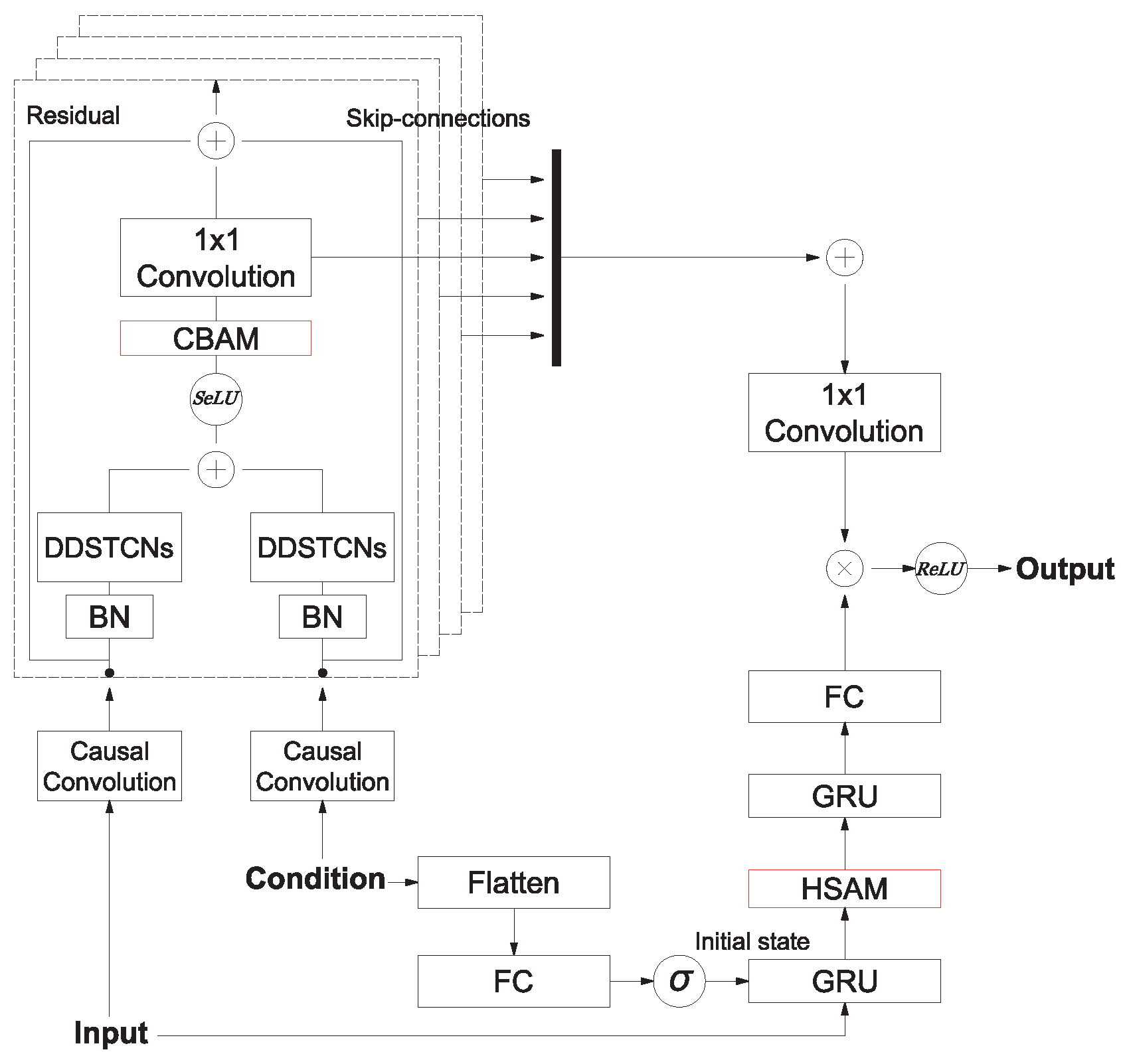
  • We introduce the conditioning methods for CNN and RNN and propose a lightweight hidden state attention module (HSAM) on RNN layers.
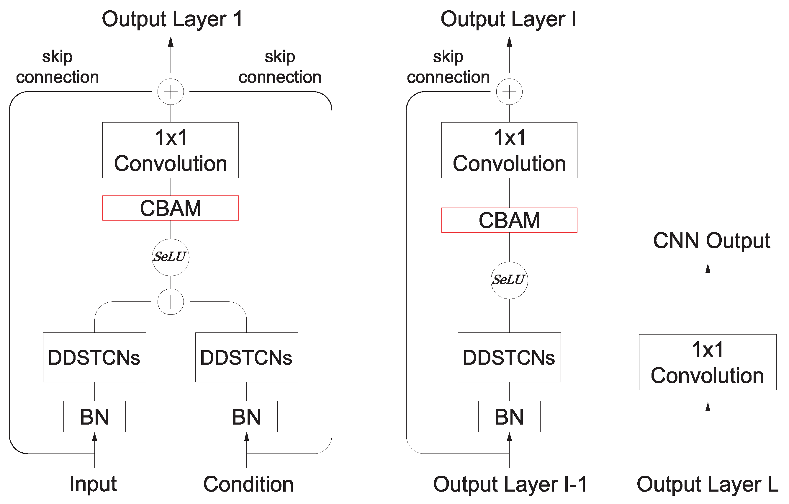
  • We have utilized the attention mechanisms in SeriesNet and present an attention-based SeriesNet combined CBAM [9] on convolutional layers and HSAM on RNN layers for time series forecasting.
  • We used GRU and DDSTCNs instead of LSTM and DC-CNN of SeriesNet to reduce the parameters in neural network layers.
The related work is shown in Section 2. Section 3 introduces the details of attention-based SeriesNet. Section 4 gives the experimental results, followed by the conclusion in Section 5.

2. Related Work

With the development of modern time series forecasting, the traditional forecasting methods such as the autoregressive integrated moving average (ARIMA) [10] model and the support vector regression (SVR) [11] have encountered a bottleneck. The model based on the artificial neural network (ANN) [12] is a further prediction approach. A single neuron in a neural network has a simple ability to reflect the essential characteristics of non-linearity. The self-organizing and compounding of these basic units enables the neural network to learn the inherent law of the sequence. Zeng et al. [13] presented enhanced back-propagation neural network (ADE-BPNN) for energy consumption forecasting, which outperforms the traditional BPNN models. Hu et al. [14] proposed a new enhanced optimization model based on the bagged echo state network (ESN) improved by differential evolution algorithm to estimate energy consumption. Subsequently, they developed DeepESN [15] by introducing deep learning idea into ESN for forecasting energy consumption and wind power generation.
The recurrent neural network (RNN) [16] is a variant method of ANN applied for a sequence that the forward and backward variables have dependencies. Subsequently, the improved RNN named Long-short term memory (LSTM) [3] is proposed to deal with the gradient disappearance problem [17] when a sequence is very long. LSTM combines short-term memory with long-term memory through three gate structures to alleviate the gradient disappearance problem. Gated recurrent unit (GRU) [4] is an advance in LSTM, which keeps the same performance as LSTM while simplifying the structure of LSTM. Recently, it has been found that convolutional neural networks (CNN) [18] widely used in image recognition, is also suitable for time series forecasting. Dilated causal convolutional neural networks (DC-CNN) [2] is a variant of CNN for time series forecasting, which allows the reception field greater than the length of the filter by skipping some inputs. Dilated depthwise separable temporal convolutional networks (DDSTCNs) [5] is a further variant of DC-CNN, which divides the DC-CNN into two steps: depthwise convolution and pointwise convolution. These two steps significantly reduce the computation cost compared with a normal CNN. Shen et al. [1] proposed the SeriesNet, which contains LSTM and DC-CNN as shown in Figure 1 to extract temporal features. The SeriesNet adopts residual learning [19] and batch normalization (BN) [20] as Google waveNet [21] to improve its generalization and achieved good forecasting accuracy. The SeriesNet can directly conduct on raw time sequences. But the specific conditioning method is not introduced in Shen’s work. Borovykh et al. [22] proposed the CNN-based multi-conditional time series forecasting with excellent results. Philipperemy et al. [23] introduced the RNN-based conditioning method for additional non-temporal information.
The attention mechanism is another advance in deep learning. An attention mechanism equips a neural network with the ability to focus on a subset of its inputs. In recurrent networks, the encoder-decoder structure based attention mechanisms [6] have been proposed for time series forecasting with high accuracy. In convolutional networks, Hu et al. [24] presented a lightweight attention module, named squeeze-and-excitation networks (SeNet), which considered global average pooling as an attention mechanism for image recognition and adopted in Google ResNet [19]. The convolutional block attention module (CBAM) [9] is an improvement of SeNet by taking account of both global average and max pooling simultaneously in the channel and spatial attention modules, respectively. Nauta et al. [5] considered attention-based dilated depthwise separable temporal convolutional networks (AD-DSTCNs) and demonstrated that attention mechanisms could be successfully used in DDSTCNs for time series forecasting.

3. Structure of Attention-Based SeriesNet

This paper improves Shen’s work [1] by using two different attention mechanisms on two sub-networks of SeriesNet, respectively. The first subnet utilizes CBAM-based DDSTCNs to instead of DC-CNN [2] to learn short interval features. The stacked deep residual connection blocks [19] with different dilated rates can learn long interval features with different reception fields. The batch normalization (BN) [20] is added to solve the gradient vanishing problem. For the second subnet, HSAM-based GRU is applied instead of LSTM for learning the holistic features followed by a full connection (FC) layer to set the output dimensionality. Finally, the outputs of two sub-networks will be element-wise multiplied together for time series forecasting. The attention-based SeriesNet can directly conduct on the raw time series by conditioning methods.

3.1. Conditioning

According to [21,22], given a one-dimensional time series with T time steps x = { x 1 , x 2 , , x T } R 1 × T , the object is to output the next value x t conditional on the series’ history, x 1 , , x t 1 by maximizing the likelihood function as below:
p ( h ) = t = 1 T p ( x t | x 1 , x 2 , , x t 1 ) .
The distribution of one time series conditional on additional time series y R i × T is given by
p ( x | y ) = t = 1 T p ( x t | x 1 , x 2 , , x t 1 , y ) ,
This paper first adopts a causal convolution to map the input and the condition (additional time series) with the same feature dimension (channel). Then the CNN-based conditioning method [22] is done by computing the activation function of the convolution as:
S e L U ( f d 1 × k ( x ) + f d 1 × h ( y ) ) ,
where f d 1 × k and f d 1 × h denotes the convolution operation with filter size 1 × k , 1 × h and dilation rate d in the depthwise convolution of DDSTCNs, respectively. The conditioning method for CNN is similar to Borovykh’s work [22] except for the activation function. This paper adopts the scaled exponential linear unit (SeLU) [25] instead of the rectified linear unit (ReLU) [26] since the self-normalizing properties of the SeLU has more robust representations of the time series. As shown in Figure 2, the input and condition are conditioned in the first residual layer (L), followed by the CBAM [9] and the 1 × 1 convolution, and summed with the parametrized skip connections. The result from this layer is the input in the subsequent convolution layer with a residual connection, which is repeated to obtain the output from layer L and forwarded to a 1 × 1 convolution to generate the final CNN output.
This paper presents the conditioning method for RNN based on Philipperemy’s [23] work as demonstrated in Figure 3. The given multi-conditions y R i × T is considered as the initial state of the first RNN layer by transforming its shape into y R p × m , where m is the unit number of the first RNN layer and p’s value is 1 or 2 for GRU and LSTM, respectively. Since LSTM owns hidden state and cell state, GRU only has hidden state. In case of GRU, the flatten operation is implemented on y R i × T to convert its shape into y R 1 × v , where v is the product of i and T. The FC layer with a sigmoid activation function is followed with the flatten operation to obtain the target shape y R 1 × m . For LSTM, this paper first adopts flatten operation followed by a FC layer with a sigmoid activation function to transform the shape of y R i × T into y R 1 × 2 m , and then reshapes it into y R 2 × m . Each row of y R 2 × m is considered as the initial hidden state and initial cell state, respectively. This approach naturally solves the shape problem of multi-conditions, and also avoids polluting the inputs with additional information.

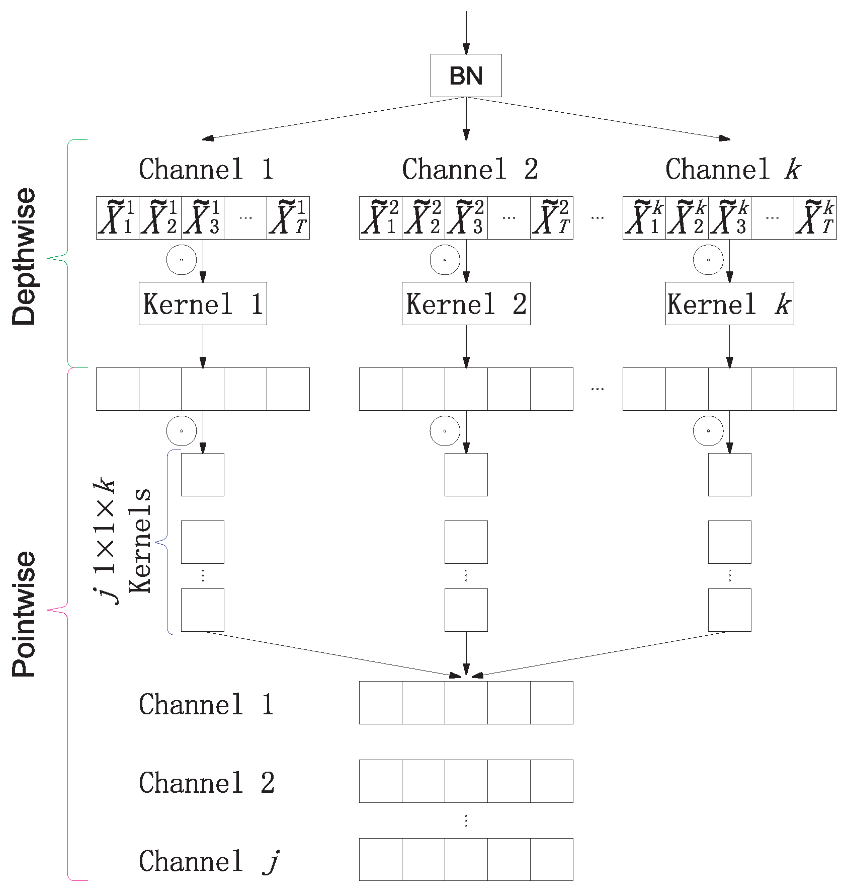
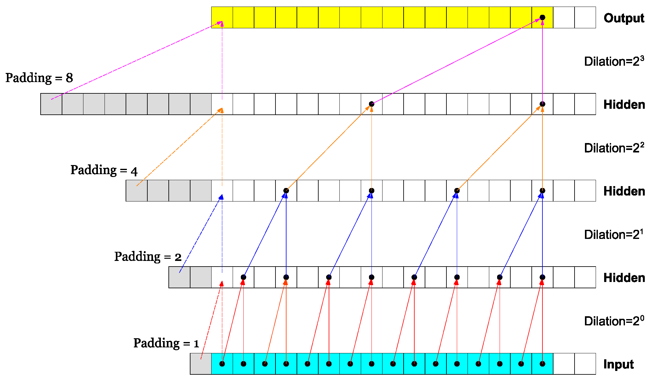
3.2. Dilated Depthwise Separable Temporal Convolutional Networks

The DDSTCNs introduced in [5] based on the depthwise separable convolution [27], which is well known by Google’s Xception architecture for image classification [27]. A depthwise separable convolution splits a kernel into two separate kernels that do two convolutions: the depthwise convolution and the pointwise convolution. The depthwise convolution separates the channels by applying a different kernel to each input channel. The pointwise convolution adopts a one times one kernel to each output channel of depthwise convolution and merges them together. This architecture is different from normal CNN that two convolutions improve computation performance than only one kernel per layer. The separate channels can correctly handle each dimension of input data impacts on output data, followed by a pointwise convolution tunes the number of output channels where the multiplications between parameters reduced significantly. Our architecture consists of k channels, one for each output from batch normalization (BN) [20] layer. An overview of this architecture is shown in Figure 4. Figure 5 is an example of stacked temporal DC-CNN, which explains the details of the left zero padding to predict the first values. The dilation rate 1 , 2 , 4 , , 2 n is considered in the depthwise convolution of each DDSTCNs layer to adjust the receptive field.

3.3. Convolutional Block Attention Module

The CBAM [9] adopts global average pooling and max pooling both in channel and spatial direction of a 2D image within an intermediate feature map satisfying F R C × H × W , where C , H and W denotes the channel, height and width, respectively. Figure 6 illustrates the details of channel attention module M c R C × 1 × 1 and spatial attention module M s R 1 × H × W of CBAM. For 1D time series, the height H = 1 . Given an intermediate feature map F R n × T as input, this paper uses feature dimension n and time steps T of the previous layer output instead of C and W in a image. The feature (channel) attention generates time step context descriptors F a v g n R n × 1 and F m a x n R n × 1 of a feature map by using both average and max pooling operation along the time step axis, and then fowards to a shared multi-layer perception (MLP) to produce the feature (channel) attention map M n R n × 1 as:
M n ( F ) = σ ( M L P ( A v g P o o l ( F ) ) ) + M L P ( M a x P o o l ( F ) )   = σ ( W 1 ( W 0 ( F a v g n ) ) + W 1 ( W 0 ( F m a x n ) ) ) ,
where σ indicates the sigmoid activation function, the MLP weights W 0 R n / r × n and W 1 R n × n / r respectively followed by a ReLU and sigmoid activation function are shared for both inputs. r is the reduction ratio used to reduce the parameters in W 0 . The feature attention map M n R n × 1 element-wise multiplies the intermediate feature map F R n × T to generate a new intermediate map F R n × T to feed in time step (spatial) attention module:
F = M n ( F ) F ,
where ⊗ is an element-wise multiplication. The time step (spatial) attention module generates a concatenated feature descriptor [ F a v g T ; F m a x T ] R 2 × T by applying average pooling and max pooling along the feature axis, followed by a standard convolution layer. The time step (spatial) attention map M T R 1 × T is computed as:
M T ( F ) = σ ( f 1 × 7 ( [ A v g P o o l ( F ) ; M a x P o o l ( F ) ] ) )   = σ ( f 1 × 7 ( [ F a v g T ; F m a x T ] ) ) ,
where f 1 × 7 indicates a 1 × 7 kernel size convolution operation. At last, the element-wise multiplication between M T R 1 × T and F R n × T is executed to renew the intermediate feature map as:
F = M T F F ,
where F R n × T and will be input to next layer.

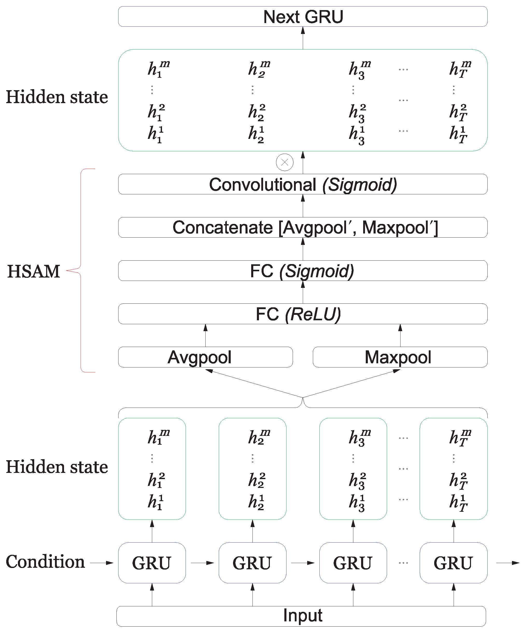
3.4. Hidden State Attention Module

This paper presents the RNN-based HSAM by integrating the two modules of CBAM together. The HSAM is implemented between every two GRU layers as illustrated in Figure 7. The GRU unit merges the memory cell state and hidden state of LSTM unit into one hidden state, and reduces the three sigmoid gates of LSTM unit to two gates: reset gate r t and update gate z t to simplify the structure. Feeding the given one-dimensional time series with T time steps x = { x 1 , x 2 , , x T } R 1 × T in a GRU layer, the update formulas of the GRU unit are summarized as:
z t = σ ( W z [ h t 1 ; x t ] ) ,
r t = σ ( W r [ h t 1 ; x t ] ) ,
h ˜ t = t a n h ( W [ r t h t 1 ; x t ] ) ,
h t = ( 1 z t ) h t 1 + z t h ˜ t ,
where h t R m × 1 is the hidden state with size m and ⊗ is an element-wise multiplication. [ h t 1 ; x t ] R ( m + n ) × 1 is a concatenation of the previous hidden state h t 1 and the current input x t . W z , W r , W R m × ( m + n ) are weight parameters to learn. The multi GRU layers utilize per time step hidden state of previous GRU layer as an input forwarding to the corresponding state of the next GRU layer. The input at each time step (feature axis) has great influence on the related hidden state output of the next GRU layer. Therefore, this paper aims to extract the average pooling and max pooling only along the hidden state feature axis of the previous GRU layer. There is an intermediate feature map h R m × T represents all hidden states of previous GRU layer. The hidden state attention produces feature context descriptors h a v g T R 1 × T and h m a x T R 1 × T through average pooling and max pooling along feature axis, and feeds them into a shared MLP layer. The outputs of the shared MLP layer are concatenated together as [ W 1 ( W 0 ( h a v g T ) ) ; W 1 ( W 0 ( h m a x T ) ) ] R 2 × T followed by a standard convolution layer to obtain the hidden state map H T R 1 × T as below:
H T ( h ) = σ ( f 1 × 7 ( [ M L P ( A v g P o o l ( h ) ) ) ; M L P ( M a x P o o l ( h ) ] ) )   = σ ( f 1 × 7 ( [ W 1 ( W 0 ( h a v g T ) ) ; W 1 ( W 0 ( h m a x T ) ) ] ) ) ,
where the MLP weights W 0 R m / r × 1 and W 1 R 1 × m / r with reduction ratio r are also followed by a ReLU and sigmoid activation function, respectively. Finally, the hidden state map H T element-wise multiplies the intermediate feature map h to produce a renewed intermediate feature map h R m × T feeding in next GRU layer:
h = H T h h .

4. Experiments

This paper uses five typical open time series datasets, including three economic data: S&P500 Index, Shanghai Composite Index, Tesla Stock Price and two temperature data: NewYork hourly temperature and Weather in Szeged as shown in Table 1 to evaluate the models. The attention-based SeriesNet is compared with the SeriesNet [1], the Augmented WaveNet [22], the SVR [11] and the GRU networks [4]. Each model is evaluated by 4 metrics: the root-mean-square error (RMSE), the mean absolute error (MAE), the coefficient of determination ( R 2 ) and the computation time of specific epoch numbers. This paper takes an average of ten times of training results as the final accuracy of each model.
This section uses A_SeriesNet and WaveNet instead of the attention-based SeriesNet and the augmented WaveNet for short. The experiments are executed on Windows 10 with 2.50 GHz Intel Core i7 and 8 GB memory and conducted on the python environment with Keras deep learning structure. The hyper-parameters of A_SeriesNet shown in Table 2, Table 3 and Table 4 are slightly adjusted when it applies to different datasets. The reduction ratio of CBAM and HSAM shown in Table 3 and Table 4 is one. The padding of depthwise convolution and pointwise convolution of DDSTCNs is causal and valid, respectively. In the case of three economic datasets, this paper uses daily average stock price as the target time series (Input) by taking the average of daily high and low stock price. The part of the other time series in two economic datasets, such as the daily trading volume and the daily close stock price, is chosen as the conditions. For the two temperature datasets, the temperature is considered as the target time series (Input), the Dew point and the humidity are chosen as the conditions. This paper adopts the MAE as the loss function as below:
l o s s m i n = 1 T t = 1 T F t A t ,
where F t and A t denotes the target value and predicted value at time t, respectively. The weights of all CNN layers of A_SeriesNet are initialized with a truncated normal distribution with zero mean and constant variance of 0.05. The GRU layers of A_SeriesNet are initialized with he_normal distribution. The Adam optimizer [28] is used with the learning rate 0.001 and β 1 of 0.9. The related layer numbers of SeriesNet and WaveNet are unified with A_SeriesNet as shown in Table 2. This paper removed CBAM and HSAM and used DC-CNN and LSTM instead of DDSTCNs and GRU in Figure 3 as the conditional structure of SeriesNet. All the models except for SVR used the conditioning method for the experiments.
This paper computes each layer’s complexity for detecting our model’s computational performance, as demonstrated in Table 2, Table 3 and Table 4. The shape of input time series and condition is respectively specified to x R 1 × T and y R 1 × T for easy calculating the complexity. The evaluation is only limited to the forward propagation of the computational process. The complexity of a standard 1D CNN layer [29] is defined as below:
C o m p l e x i t y O ( M · K · C i n · C o u t ) ,
where M is the width of the output feature map, K denotes the width of the kernel, C i n and C o u t represents the channel input and channel output, respectively. We ignore the bias of all CNN layers and full connection layers for convenience to compute the complexity. The complexity of a 1D DDSTCNs layer is computable as follows:
C o m p l e x i t y O ( M · K · C i n + M · C i n · C o u t ) .
On the other hand, LSTM is local in space and time [3], which means that the input length does not affect the storage requirements of the network and for each time step, the time complexity per weight is O ( 1 ) . Therefore, the overall complexity of an LSTM per time step is equal to O ( w ) , where w is the number of weights. The complexity of a standard LSTM layer per time step is calculated as:
C o m p l e x i t y O ( 4 · ( I · H + H 2 + H ) ) ,
where I denotes the dimension of input data, H represents the hidden unit numbers. The Complexity of a standard GRU layer per time step is simpler than LSTM, which is given as:
C o m p l e x i t y O ( 3 · ( I · H + H 2 + H ) ) .
The overall complexity of our model is the sum of the complexity of all layers.
Table 5 shows the experimental results when the forecast sliding window representing the future time span is 1. GRU 20 2 denotes using 2 layers of GRU cell and each layer contains 20 neurons. The A_SeriesNet has the best performance on both non-linear and non-stationary economic datasets and relatively stationary time series temperature dataset compared with the other models. The lower RMSE, MAE and higher R 2 close to 1 means better model fitting. This paper performs the models except for SVR for 64 epochs with 64 mini-batch size one time. This epoch number allows the models to achieve a satisfactory convergence on five datasets.
Table 6 demonstrates the average computation time (in seconds) of the models for one-time training. The computation time of A_SeriesNet is in rank 3, which is faster than SeriesNet and slower than GRU 20 2 . The SVR takes longer training time to obtain the results close to the other models.
Table 7 shows the results of GRU combined with HSAM (HSAM_GRU) compared with GRU. This paper adopts GRU 20 2 with 2 layers of GRU cell and each layer contains 20 neurons and GRU 20 4 with 4 layers of GRU cell and each layer contains 20 neurons for the experiments. The results show that the different layers of HSAM_GRU are superior to related GRU networks. When the number of layers increased, the accuracy of GRU for 5 datasets decreases. HSAM can keep the accuracy of deep GRU networks. The computation time of HSAM_GRU is close to GRU as demonstrated in Table 8.
Table 9, Table 10 and Table 11 show the hyper parameters and complexity of SeriesNet and WaveNet in our experiments. The shape of input time series and condition in the tables is also appointed to x R 1 × T and y R 1 × T , respectively. We also ignore the bias of all CNN layers and full connection layers for computing the overall complexity of these models. The structure of GRU 20 4 is similar to GRU 20 2 in Table 10 and Table 12 gives the complexity comparison results of deep learning models. The complexity of our model is between GRU 20 2 and SeriesNet.

5. Conclusions

This paper proposed a deep learning neural network structure named attention-based SeriesNet, which desires to predict the future value of time series. The attention-based SeriesNet applies DDSTCNs and GRU instead of DC-CNN and LSTM in SerieNet to accelerate the training. Furthermore, this model adopts CBAM attention on residual learning module and proposed HSAM attention on GRU networks to better extract the potential features from the input time series. We succeeded in improving SeriesNet since our model’s accuracy, and complexity is superior to the SeriesNet. The experiment results also show that attention-based SeriesNet has higher forecasting accuracy than other models. This paper only explored the performance of the SeriesNet models on the economic and temperature datasets. Further analysis of different types of datasets is required to examine the capability of attention-based SeriesNet to forecast from different data distributions for varying forecast horizons. This paper didn’t evaluate the performance of hidden state attention mechanisms on recurrent neural networks with deep structure. The only two or four layers GRU can not adequately describe its performance. It was also found that the forecasts were very sensitive to layer weight initialization, receptive field and training duration. The parameter tuning is necessary for different datasets.

6. Future Work

In the future, we will continue to develop the attention mechanism of our model. The dual-stage attention-based recurrent neural network has good accuracy in the field of time series forecasting. The dual-stage attention structure, combined with a hidden state attention module, may improve our model’s performance. This paper only detected the conditional time series for time series forecasting. The performance of our model for multi-variable time series will also be detected in the future.

Author Contributions

Conceptualization, Y.C.; software, Y.C. and Z.L.; validation, Y.C. and Z.L.; formal analysis, Y.C. and Z.L.; data curation, Y.C. and Z.L.; writing–original draft, Y.C. and Y.M.; writing–review and editing, Y.C. and Y.M.; supervision, Y.M. All authors have read and agreed to the published version of the manuscript.

Funding

This research received no external funding.

Acknowledgments

This work is partially supported by KAKENHI (16K00155, 17H01823) Japan.

Conflicts of Interest

The authors declare no conflict of interest.

References

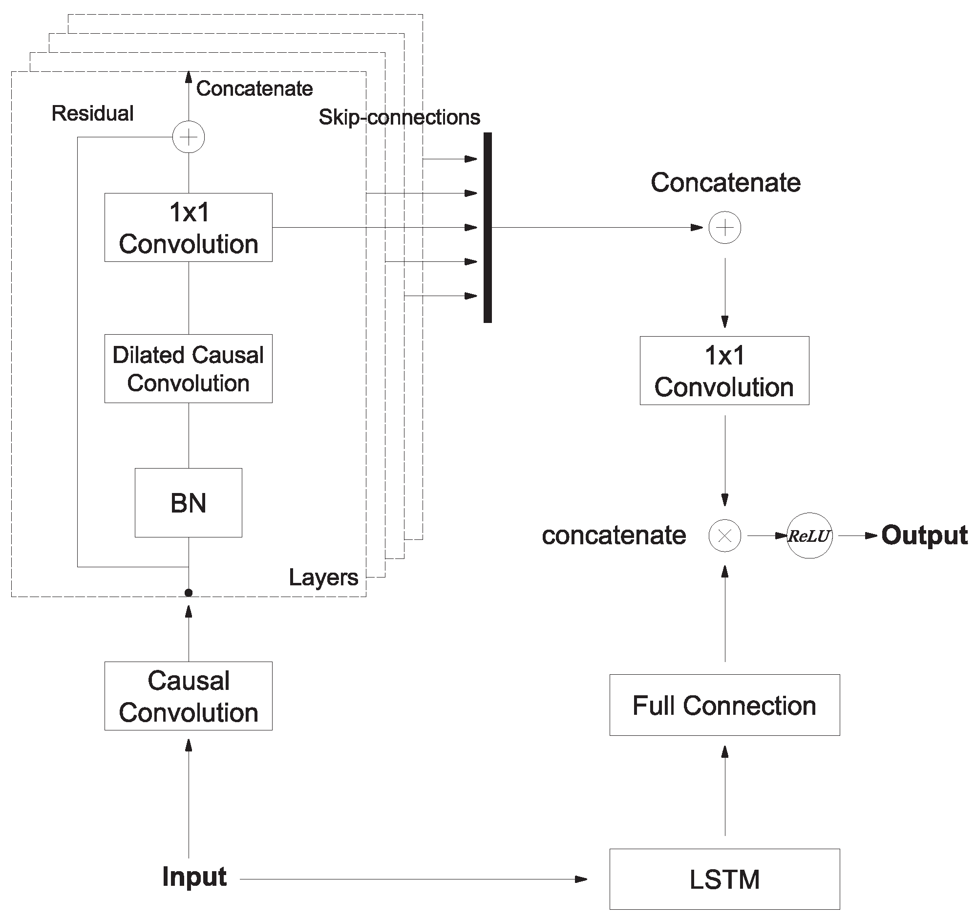
  1. Shen, Z.; Zhang, Y.; Lu, J.; Xu, J.; Xiao, G. SeriesNet: A Generative Time Series Forecasting Model. In Proceedings of the 2018 International Joint Conference on Neural Networks (IJCNN), Rio de Janeiro, Brazil, 8–13 July 2018; pp. 1–8. [Google Scholar]
  2. Borovykh, A.I.; Bohte, S.M.; Oosterlee, C.W. Dilated convolutional neural networks for time series forecasting. J. Comput. Financ. 2019, 22, 73–101. [Google Scholar] [CrossRef] [Green Version]
  3. Hochreiter, S.; Schmidhuber, J. Long short-term memory. Neural Comput. 1997, 1735–1780. [Google Scholar] [CrossRef] [PubMed]
  4. Chung, J.; Gulcehre, C.; Cho, K.; Bengio, Y. Empirical evaluation of gated recurrent neural networks on sequence modeling. arXiv 2014, arXiv:1412.3555v1. [Google Scholar]
  5. Nauta, M.; Bucur, D.; Seifert, C. Causal Discovery with Attention-Based Convolutional Neural Networks. Mach. Learn. Knowl. Extr. 2019, 1, 312–340. [Google Scholar] [CrossRef] [Green Version]
  6. Qin, Y.; Song, D.; Cheng, H.; Cheng, W.; Jiang, G.; Cottrell, G. A Dual-Stage Attention-Based Recurrent Neural Network for Time Series Prediction. In Proceedings of the 26th International Joint Conference on Artificial Intelligence (IJCAI’17); AAAI Press: Palo Alto, CA, USA, 2017; pp. 2627–2633. [Google Scholar]
  7. Yagmur, G.C.; Hamid, M.; Parantapa, G.; Eric, G.; Ali, A.; Vadim, S. Position-Based Content Attention for Time Series Forecasting with Sequence-to-Sequence RNNs. In Proceedings of the Neural Information Processing: 24th International Conference, ICONIP 2017, Guangzhou, China, 14–18 November 2017; pp. 533–544. [Google Scholar]
  8. Luong, T.; Pham, H.; Manning, C.D. Effective Approaches to Attention-based Neural Machine Translation. In Proceedings of the 2015 Conference on Empirical Methods in Natural Language Processing, Lisbon, Portugal, 17–21 September 2015; pp. 1412–1421. [Google Scholar]
  9. Woo, S.; Park, J.; Lee, J.Y.; Kweon, I.S. CBAM: Convolutional Block Attention Module; Ferrari, V., Hebert, M., Sminchisescu, C., Weiss, Y., Eds.; ECCV 2018, Lecture Notes in Computer Science; Springer: Cham, Switzerland, 2018; Volume 11211, pp. 3–19. [Google Scholar]
  10. Liu, C.; Hoi, S.C.H.; Zhao, P.; Sun, J. Online ARIMA algorithms for time series prediction. In Proceedings of the Thirtieth AAAI Conference on Artificial Intelligence (AAAI’16); AAAI Press: Palo Alto, CA, USA, 2016; pp. 1867–1873. [Google Scholar]
  11. Drucker, H.; Burges, C.J.C.; Kaufman, L.; Smola, A.; Vapnik, V. Support vector regression machines. In Proceedings of the 9th International Conference on Neural Information Processing Systems (NIPS’96); MIT Press: Cambridge, MA, USA, 1996; pp. 155–161. [Google Scholar]
  12. Mishra, M.; Srivastava, M. A view of Artificial Neural Network. In Proceedings of the 2014 International Conference on Advances in Engineering & Technology Research (ICAETR-2014), Unnao, India, 1–2 August 2014; pp. 1–3. [Google Scholar]
  13. Zeng, Y.; Zeng, Y.; Choi, B.; Wang, L. Multifactor-influenced energy consumption forecasting using enhanced back-propagation neural network. Energy 2017, 127, 381–396. [Google Scholar] [CrossRef]
  14. Hu, H.; Wang, L.; Peng, L.; Zeng, Y. Effective energy consumption forecasting using enhanced bagged echo state network. Energy 2020, 193, 116778. [Google Scholar] [CrossRef]
  15. Hu, H.; Wang, L.; Lv, S. Forecasting energy consumption and wind power generation using deep echo state network. Renew. Energy 2020, 154, 598–613. [Google Scholar] [CrossRef]
  16. Sherstinsky, A. Fundamentals of Recurrent Neural Network (RNN) and Long Short-Term Memory (LSTM) network. arXiv 2020, arXiv:1808.03314. [Google Scholar] [CrossRef] [Green Version]
  17. Pascanu, R.; Mikolov, T.; Bengio, Y. On the difficulty of training recurrent neural networks. Int. Conf. Int. Conf. Mach. Learn. 2013, 28, 1310–1318. [Google Scholar]
  18. Krizhevsky, A.; Sutskever, I.; Hinton, G.E. ImageNet classification with deep convolutional neural networks. Commun. ACM 2017, 60, 84–90. [Google Scholar] [CrossRef]
  19. He, K.; Zhang, X.; Ren, S.; Sun, J. Deep Residual Learning for Image Recognition. In Proceedings of the 2016 IEEE Conference on Computer Vision and Pattern Recognition (CVPR), Las Vegas, NV, USA, 27–30 June 2016; pp. 770–778. [Google Scholar]
  20. Ioffe, S.; Szegedy, C. Batch normalization: Accelerating deep network training by reducing internal covariate shift. Int. Conf. Int. Conf. Mach. Learn. 2015, 37, 448–456. [Google Scholar]
  21. Van Den Oord, A.; Dieleman, S.; Zen, H.; Simonyan, K.; Vinyals, O.; Graves, A.; Kalchbrenner, N.; Senior, A.; Kavukcuoglu, K. Wavenet: A generative model for raw audio. arXiv 2016, arXiv:1609.03499. [Google Scholar]
  22. Borovykh, A.; Bohte, S.M.; Oosterlee, C.W. Conditional time series forecasting with convolutional neural networks. arXiv 2017, arXiv:1703.04691v5, 729–730. [Google Scholar]
  23. Philipperemy, R. Conditional RNN (Tensorflow Keras). GitHub Repository. 2020. Available online: https://github.com/philipperemy/cond_rnn (accessed on 4 June 2020).
  24. Hu, J.; Shen, L.; Sun, G. Squeeze-and-Excitation Networks. In Proceedings of the 2018 IEEE/CVF Conference on Computer Vision and Pattern Recognition, Salt Lake City, UT, USA, 18–22 June 2018; pp. 7132–7141. [Google Scholar]
  25. Klambauer, G.; Unterthiner, T.; Mayr, A.; Hochreiter, S. Self-Normalizing Neural Networks. arXiv 2017, arXiv:1706.02515. [Google Scholar]
  26. Abien, F.A. Deep Learning using Rectified Linear Units (ReLU). arXiv 2018, arXiv:1803.08375v2. [Google Scholar]
  27. Chollet, F. Xception: Deep Learning with Depthwise Separable Convolutions. In Proceedings of the 2017 IEEE Conference on Computer Vision and Pattern Recognition (CVPR), Honolulu, HI, USA, 21–26 July 2017; pp. 1800–1807. [Google Scholar]
  28. Kingma, D.P.; Jimmy, B. Adam: A Method for Stochastic Optimization. arXiv 2014, arXiv:1412.6980. [Google Scholar]
  29. Tsironi, E.; Barros, P.; Weber, C.; Wermter, S. An analysis of Convolutional Long Short-Term Memory Recurrent Neural Networks for gesture recognition. Neurocomputing 2017, 268, 76–86. [Google Scholar] [CrossRef]
Figure 1. The structure of the SeriesNet.
Information 11 00305 g001
Figure 2. The structure of the conditional CNN sub-networks.
Information 11 00305 g002
Figure 3. The structure of the attention-based SeriesNet.
Information 11 00305 g003
Figure 4. The structure of the DDSTCNs.
Information 11 00305 g004
Figure 5. The structure of the DC-CNN.
Information 11 00305 g005
Figure 6. The overview of CBAM.
Information 11 00305 g006
Figure 7. The overview of HSAM.
Information 11 00305 g007
Table 1. Time series dataset.
Time SeriesTime RangeTrain DataValidation DataTest Data
S&P500 Index1950.01–2015.123297320320
Shanghai Composite Index2004.01–2019.062430280280
Tesla Stock Price2010.06–2017.031049160160
NewYork temperature2016.01–2016.072430320320
Weather in Szeged2006.04–2016.091700240240
Table 2. Hyper parameters and complexity of attention-based SeriesNet.
TypeUnits/FiltersSizeDilation RatePaddingOutputComplexity
Conv1D(Input)1301causal(50, 1)1500
BN (50, 1)0
DDSTCNs871causal/valid(50, 8)750
Conv1D(Condition)1201causal(50, 1)1000
BN (50, 1)0
DDSTCNs841causal/valid(50, 8)600
Add (50, 8)0
SeLU (50, 8)0
CBAM (50, 8)956
Conv1D111same(50, 1)400
Add (50, 1)0
BN (50, 1)0
DDSTCNs872causal/valid(50, 8)750
SeLU (50, 8)0
CBAM (50, 8)956
Conv1D111same(50, 1)400
Add (50, 1)0
BN (50, 1)0
DDSTCNs8716causal/valid(50, 8)750
SeLU (50, 8)0
CBAM (50, 8)956
Conv1D111same(50, 1)400
Add(Skip-Connection) (50, 1)0
Conv1D111same(50, 1)50
Condition (1, 20)1000
GRU(Input, Condition)20 (50, 20)66,000
HSAM (50, 20)780
GRU20 (50, 20)123,000
FC1 (50, 1)20
Multiply (50, 1)0
ReLU (50, 1)0
Total 204,480
Table 3. Hyper parameters and complexity of HSAM.
TypeUnits/FiltersSizeDilation RatePaddingOutputComplexity
Lambda_Mean(GRU) (50, 1)0
FC20 (50, 20)20
ReLU (50, 20)0
FC1 (50, 1)20
Lambda_Max(GRU) (50, 1)0
FC20 (50, 20)20
ReLU (50, 20)0
FC1 (50, 1)20
Concatenate (50, 2)0
Conv1D171same(50, 1)700
Sigmoid (50, 1)0
Multiply(GRU, Sigmoid) (50, 20)0
Total 780
Table 4. Hyper parameters and complexity of CBAM.
TypeUnits/FiltersSizeDilation RatePaddingOutputComplexity
GlobalAvgPooling1D(SeLU) (1, 8)0
FC8 (1, 8)64
ReLU (1, 8)0
FC8 (1, 8)64
GlobalMaxPooling1D(SeLU) (1, 8)0
FC8 (1, 8)64
ReLU (1, 8)0
FC8 (1, 8)64
Add (1, 8)0
Sigmoid (1, 8)0
Multiply1(SeLU, Sigmoid) (50, 8)0
Lambda_Mean(Multiply1) (50, 1)0
Lambda_Max(Multiply1) (50, 1)0
Concatenate (50, 2)0
Conv1D171same(50, 1)700
Sigmoid (50, 1)0
Multiply2(Multiply1, Sigmoid) (50, 8)0
Total 956
Table 5. The result of accuracy comparison.
Time SeriesA_SeriesNetSeriesNetWaveNet GRU 20 2 SVR
RMSEMAE R 2 RMSEMAE R 2 RMSEMAE R 2 RMSEMAE R 2 RMSEMAE R 2
S&P500 Index8.907.170.9810.088.110.9711.138.730.9710.578.390.9716.1612.610.96
Shanghai Composite Index56.6936.490.9871.9655.500.9780.5260.100.9779.2950.170.9782.2563.190.97
Tesla Stock Price4.563.360.974.823.680.965.504.360.955.594.380.954.743.360.96
NewYork temperature1.631.200.971.681.220.971.761.250.961.721.250.971.791.230.96
Weather in Szeged1.220.710.961.290.790.961.440.900.951.420.880.951.410.830.95
Table 6. The result of performance comparison.
Time SeriesA_SeriesNetSeriesNetWaveNet GRU 20 2 SVR
S&P500 Index100.80103.6217.9974.37273.49
Shanghai Composite Index92.7294.4218.7376.10237.40
Tesla Stock Price61.9064.6936.3641.37124.97
NewYork temperature99.78101.3817.8074.73107.08
Weather in Szeged89.2496.5617.5462.93115.96
Table 7. The accuracy comparison of HSAM_GRU and GRU.
Time SeriesHSAM_ GRU 20 2 GRU 20 2 HSAM_ GRU 20 4 GRU 20 4
RMSEMAE R 2 RMSEMAE R 2 RMSEMAE R 2 RMSEMAE R 2
S&P500 Index9.517.770.9810.578.390.9710.188.010.9712.239.920.96
Shanghai Composite Index78.4448.490.9779.2950.170.9780.4654.740.9792.8366.700.96
Tesla Stock Price5.023.890.965.594.380.956.244.630.946.295.000.94
NewYork temperature1.681.230.971.721.250.971.731.270.971.761.280.97
Weather in Szeged1.330.800.961.420.880.951.410.820.951.561.000.94
Table 8. The performance comparison of HSAM_GRU and GRU.
Time SeriesHSAM_ GRU 20 2 GRU 20 2 HSAM_ GRU 20 4 GRU 20 4
S&P500 Index81.9474.37167.42145.09
Shanghai Composite Index82.8776.10172.13141.04
Tesla Stock Price39.4436.3686.8276.52
NewYork temperature81.2174.73170.77147.92
Weather in Szeged66.2062.93125.95117.07
Table 9. Hyper parameters and complexity of augmented WaveNet.
TypeUnits/FiltersSizeDilation RatePaddingOutputComplexity
Conv1D(Input)871causal(50, 8)2800
ReLU (50, 8)0
Conv1D(Condition)871causal(50, 8)2800
ReLU (50, 8)0
Add (50, 8)0
Conv1D872causal(50, 8)22,400
ReLU (50, 8)0
Add (50, 8)0
Conv1D8716causal(50, 8)22,400
ReLU (50, 8)0
Add(Skip-Connection) (50, 8)0
Conv1D111same(50, 1)400
Total 95,600
Table 10. Hyper parameters and complexity of GRU 20 2 .
TypeUnits/FiltersSizeDilation RatePaddingOutputComplexity
Condition (1, 20)1000
GRU(Input, Condition)20 (50, 20)66,000
GRU20 (50, 20)123,000
FC1 (50, 1)20
Total 190,020
Table 11. Hyper parameters and complexity of SeriesNet.
TypeUnits/FiltersSizeDilation RatePaddingOutputComplexity
Conv1D(Input)1201causal(50, 1)1000
BN (50, 1)0
Conv1D871causal(50, 8)2800
Conv1D(Condition)1201causal(50, 1)1000
BN (50, 1)0
Conv1D841causal(50, 8)1600
Add (50, 8)0
Conv1D111same(50, 1)400
Add (50, 1)0
BN (50, 1)0
Conv1D872causal(50, 8)2800
Conv1D111same(50, 1)400
Add (50, 1)0
BN (50, 1)0
Conv1D8716causal(50, 8)2800
Conv1D111same(50, 1)400
Add(Skip-Connection) (50, 1)0
Conv1D111same(50, 1)50
Condition (2, 20)2000
LSTM(Input, Condition)20 (50, 20)88,000
LSTM20 (50, 20)164,000
FC1 (50, 1)20
Multiply (50, 1)0
ReLU (50, 1)0
Total 273,670
Table 12. The result of complexity comparison.
A_SeriesNetSeriesNetWaveNet GRU 20 2 GRU 20 4
Complexity204,480273,67095,600190,020436,020

