An Innovative Acoustic Rain Gauge Based on Convolutional Neural Networks ^†

Abstract

An accurate estimate of rainfall levels is fundamental in numerous application scenarios: weather forecasting, climate models, design of hydraulic structures, precision agriculture, etc. An accurate estimate becomes essential to be able to warn of the imminent occurrence of a calamitous event and reduce the risk to human beings. Unfortunately, to date, traditional techniques for estimating rainfall levels present numerous critical issues. The algorithm applies the Convolution Neural Network (CNN) directly to the audio signal, using 3 s sliding windows with an offset of only 100 milliseconds. Therefore, by using low cost and low power hardware, the proposed algorithm allows implementing critical high rainfall event alerting mechanisms with short response times and low estimation errors. More specifically, this paper proposes a new approach to rainfall estimation based on the classification of different acoustic timbres that rain produces at different intensities and on CNN. The results obtained on seven classes ranging from “No rain” to “Cloudburst” indicate an average accuracy of 75%, which rises to 93% if the misclassifications of the adjacent classes are not considered. Some application contexts concern smart cities for which the integration of an audio sensor inside the luminaire of a street lamp is foreseen, precision agriculture, as well as highway safety, by minimizing the risks of aquaplaning.

1. Introduction

The sudden climate change, which has taken place in recent years, has generated calamitous phenomena linked to hydrogeological instability in many areas of the world. The main existing rainfall level measurement methods employ rain gauges, weather radars and satellites [1,2,3]. The rain gauge is probably the most common rainfall measurement device, as it is able to provide an average accurate estimate of the rainfall with a precise temporal resolution; in fact, rain gauges continuously record the level of precipitation even within short time intervals. Modern tilt rain gauges consist of a plastic manifold balanced on a pin. When it tips, it actuates a switch which is then electronically recorded or transmitted to a remote collection station. Unfortunately, tipping buckets tend to underestimate the amount of rainfall, particularly in snowfall and heavy rainfall events. Moreover, they are also sensitive to the inclination of the receiver and different types of dirt that may clog the water collection point.

Many studies have been carried out regarding the classification of rainfall levels using alternative methods, parameters, and signals such as video, audio, and radio signals [4,5,6].

In [7], rain is estimated through acoustic sensors and Android smartphones. Using this system has several advantages: access to the data collected via the device’s microphone or camera; data can be sent via radio functions (WI-FI, GSM, LTE, etc.); and the cost-effectiveness of Android devices compared to high-precision meteorological instruments.

The audio data collected by the smartphone microphone are then processed to extract the fundamental parameters to be compared with the critical thresholds, and exceeding these thresholds, translates into sending an “alarm”. In addition, historical data are stored on a web server allowing remote access to information. From the audio sequence sampled at 22.05 KHz the calculation of the signal strength (dB) is performed every 5 s. To verify the validity of the results obtained with this method, measurements were carried out simultaneously with the aid of a tilting rain gauge so that the data of the two solutions can be compared.

The study carried out in [8], aims at the digital representation of rain scenes as a function of the real sounds produced by the precipitation. The research is based on the study of rainfall phenomena proposed by Marshall and Palmer, providing the frame for describing the probability distribution of the number and size of raindrops in a space of known volume, evaluating the intensity of the event, and the fact that the speed of a water drop is only related to its size.

Based on these considerations, it is possible to extract parameters relating to raindrops, useful for creating an animated digital scene. A rainy phenomenon can be modelled according to the Marshall–Palmer distribution which allows determining the relationship between the number and size of the drops in a volume as a function of the level of intensity (mm/h) obtainable from the audio recordings of actual rainfall. These were obtained using a smartphone and employing the same previously described procedure [7], but with sampling at a frequency of 44.10 KHz and, simultaneously, carrying out measurements using a rain gauge. In order to extract the frequency characteristics, various rainfall recordings of different intensity were taken and, for each, the Fourier transform was performed. One of the most evident results is that the samples in the spectrum present a high level of correlation and the high frequency components increase as the intensity of the precipitation increases. This can be interpreted by the Marshall–Palmer distribution, in fact, the number of occurring raindrops per unit of volume increases as the intensity of the rain increases, the average landing time of the drop is reduced and, consequently, the frequency of sounds increases.

The input sounds were taken from a data set, randomly selecting eight 1-s sound segments for each data, with 15 types of rainfall intensity. Once the level of rainfall has been determined, it is possible to trace the following parameters: size of the rain particles, number of drops, and falling speed.

In [9], a technique of automated learning was studied through machine learning, employing a series of functions for the classification of acoustic recordings, in order to improve the performance of the rain classification system. The classification was implemented using a ‘decision tree’ classifier and comparing this with other classifiers.

Another technique used, was a machine learning approach of analysis and classification in which the sound classes to be analyzed are defined in advance [10]. Another study carried out in [11], involved the use of frequency domain functions to represent audio input and multilabel neural networks to detect multiple and simultaneous sound events in a real recording.

Aiming to overcome some limitations present in traditional techniques to signal classification, in [12] we proposed an acoustic rain gauge based on convolutional neural network (CNN), in order to obtain accurate classification of rainfall levels. The paper presents a classification algorithm for the acoustic timbre produced by the rain in four intensities, i.e., “Weak rain”, “Moderate rain”, “Heavy rain”, and “Very heavy rain”; also the paper studies and compares the performance of an acoustic rain gauge in four different types of materials used to cover the microphone. In this study, the sound of rain was derived from the impact of water drops on a material covering the microphone. As in previous studies carried out in audio biometrics [13,14], the audio signal was analyzed using statistical variables (mean, variance and first coefficient of autocorrelation), whereas the MFCC parameters were used for the characterization of the audio spectrum.

This paper extends the previous study to a wider set of rain levels, including the “No rain” class and adding the “Shower” and “Cloudburst” rain classes. In places without a power grid (e.g., agriculture and smart roads), this system can be powered by a low-power photovoltaic panel, enabling recording at a rate proportional to the rain level, thus preserving the average lifetime of the electronic and microphone sensor components. Statistics on the average weather that characterizes a rainfall event in the territory allow us to state that the reliability and average duration of an audio rain gauge is comparable to that of a mobile terminal. The operating temperatures of an acoustic rain gauge, in fact, are the same as those of a mobile terminal. Furthermore, the microphones are designed for large temperature and humidity levels. The introduction of an acoustic rain gauge is, thus, justified, particularly, in contexts where it may be necessary to reduce the risks caused by sudden “showers” or “cloudbursts” with low operational investment, management and maintenance costs. Some application contexts concern smart cities for which is foreseen the integration of an audio sensor inside the luminaire of a street lamp, precision agriculture [15], with the advantage of being able to adapt the irrigation flows in a complementary way to different rain levels, as well as highway safety, by minimizing the risks of aquaplaning [16,17].

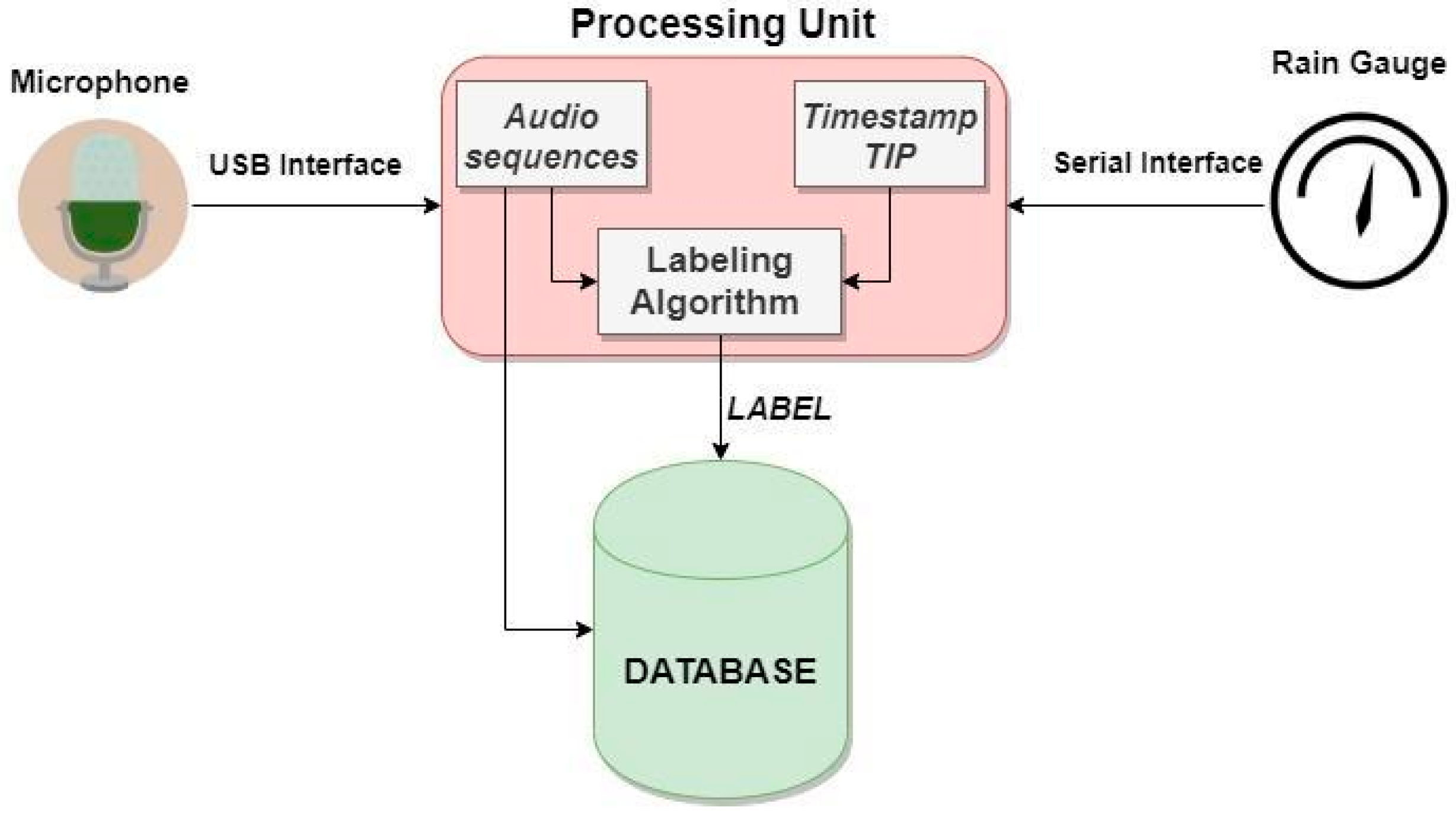
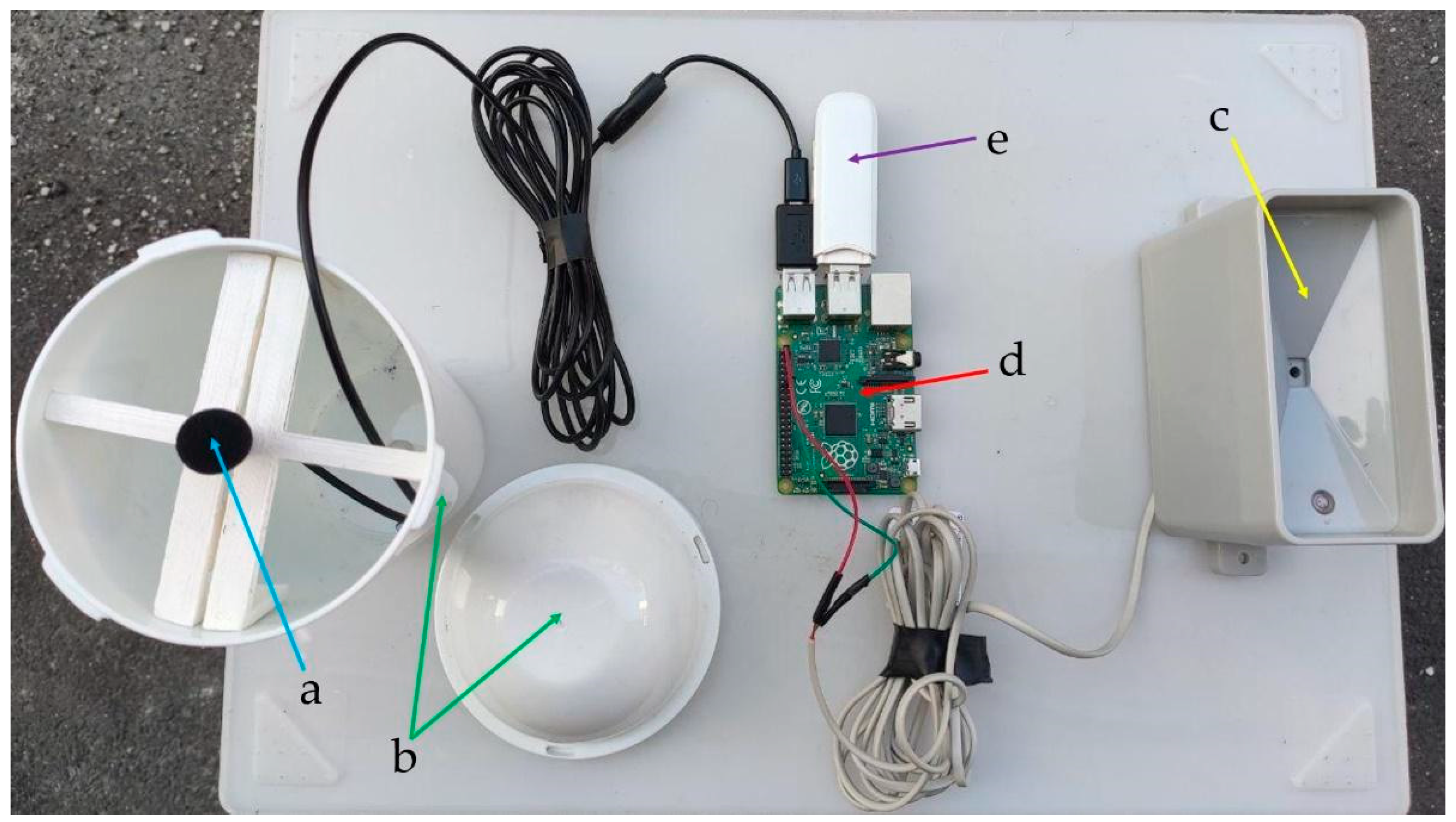
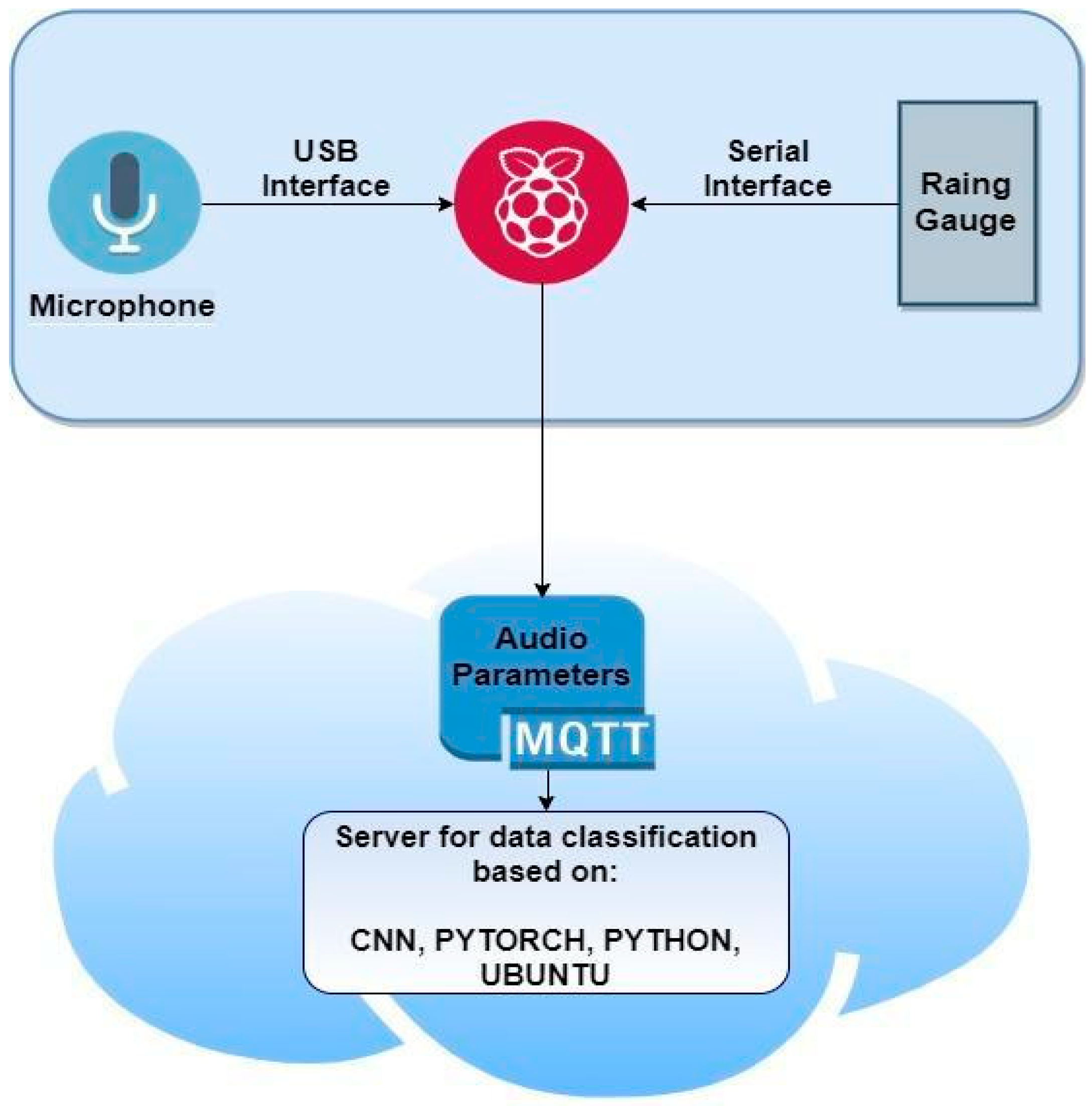
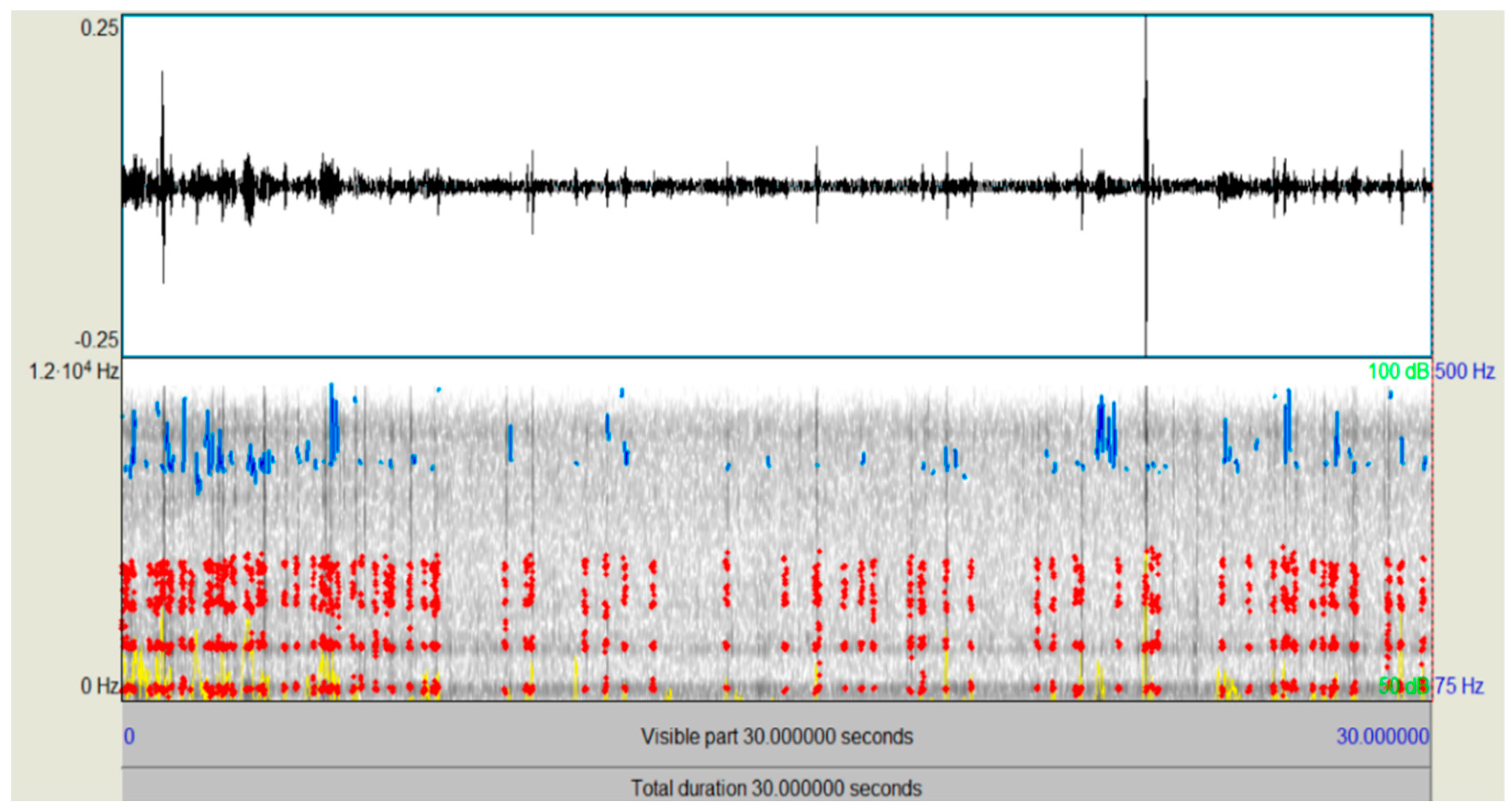
The paper is organized as follows: Section 2 illustrates the testbed scenario, i.e., database features, algorithm labeling and the types of tests carried out; Section 3 describes the hardware and software components used; Section 4 outlines the statistical and spectral analysis of the audio sequences related to different rainfall levels; Section 5 provides an overview of the Convolutional Neural Networks (CNN) used for this study; Section 6 depicts the testbed and the various performance tests and results; Section 7 suggests some ideas for future developments, whereas the last section is devoted to conclusions.

2. The Testbed Scenario

This section is devoted to defining and describing the key elements of our study, such as: database used, labeling algorithm, and testing procedure.

2.1. Database

The database was created ad hoc using the acquisition system represented in Figure 1. This system consists of a microphone and a tilting rain gauge connected to a processing unit. The processing unit houses an algorithm for labeling the audio files that allows aggregating different audio sequences in the corresponding class of precipitation intensity. Once the audio sequences are labeled in their respective intensity classes, they are entered in the database.

The acquisition system, samples audio sequences at a frequency of 22.05 KHz at 16 bit (PCM format). The database consists of seven precipitation intensity categories, defined in

Table 1. Rain classification and precipitation intensity range.

Rain Classification	Precipitation Intensity
No rain	<0.5 mm/h
Weak rain	0.5–2 mm/h
Moderate rain	2–6 mm/h
Heavy rain	6–10 mm/h
Very heavy rain	10–18 mm/h
Shower	18–30 mm/h
Cloudburst	>30 mm/h

; for each category there are 10 audio sequences each lasting 30 s.

The categories were decided upon by taking the national classification scales [18] as a reference, and slightly modifying some ranges in order to obtain a number of adequate and homogeneous examples corresponding to different classes.

The current database was created by recording the rain on five different days, some of which were characterized by the presence of different wind and environmental noise, taken at different locations, such as gardens, terraces, and countrysides, obtaining examples of all seven rainfall level classes. This implies a certain robustness of the system, since the obtained results take into account the additional external variable noise. Moreover, during the rain recording phase, continuous checks were carried out so that no dirt was created in the pan rain gauge used for labeling the rain level. Finally, through the simultaneous audio-video recording, the database was verified and cleaned up by eliminating sequences with wrong levels, through a repeated listening and contextual video verification phase.

2.2. Labeling Algorithm

Once the structure and characteristics of the adopted database are defined, it is possible to describe the labeling algorithm used for the recognition and classification of the intensity of the rain.

The preliminary requirements of the algorithm are:

• Audio file recorded in steps of X seconds;
• Timestamp of the tip, of the tipping rain gauge, stored in the database.

The characteristic parameters of the algorithm are defined below:

• $T_i$ is the final instant of the i-th time window of the audio signal;
• $C$ is the capacity, in millimeters, for the water collection of the tilting basin rain gauge;
• $R_k$ is the instant of the k-th rotation of the action frame following $T_i$;
• $R_{k-1}$ is the instant of k-th minus 1 rotation of the action frame following $T_i$;
• $T_s$ is the time interval between the two rotations of the k-th instant $R_k$ following $T_i$ and the previous instant $R_{k-1}$; and
• $T_h$ is the hour expressed in seconds, i.e., 3600 s.

The labeling algorithm is responsible for calculating the $T_s$ and subsequently, using the formula 1, we obtain the estimate of the level of precipitated rain, expressed in millimeters.

The first phase of the labeling algorithm is, therefore, the calculation of the $T_s$ which may be performed differently, based on different cases:

• 1st Case: if $R_k=0$ and $R_{k-1}=0$, we will have $T_s=0$;
• 2nd Case: if $R_{k-1}=0$ and $R_k\ne 0$, we will have $T_s=R_k-T_i$; and
• 3rd Case: if $R_{k-1}\ne 0$ and $R_k\ne 0$, we will have $T_s=R_k-R_{k-1}$.

So, once $T_s$, is obtained, the labeling algorithm is as follows:

• 1st Case: if $T_s>T_h$ the minimum estimate in mm/h is equal to 0; and
• 2nd Case: if $T_s\le T_h$ the estimate in mm/h is calculated with the following formula:

  $$e=C\times \frac{T_h}{T_s}$$

  (1)

The result of Equation (1) is compared with the rain classes, defined in Table 1, for the labeling of the audio files in the database.

2.3. Test Scenario

The tests were conducted using mainly two instruments related to the measurement of rainfall intensity: a microphone inserted into a rigid plastic shaker. The signals related to the various timbres of the rain sounds are used as the input variables of a pattern recognition system based on a CNN classifier.

The scenario is characterized by real rain which, for the total duration of the test, covered the seven rainfall intensities shown in Table 1.

3. Hardware and Software System Description

The system implemented and studied in this paper is characterized by a device capable of detecting the rain audio data, when it falls on a plastic surface. In particular, we are interested in obtaining a more efficient and faster classification of the different levels of rainfall intensity. The acoustic rain gauge, see Figure 2, is characterized by the following components:

• microphone (a);
• plastic shaker (b);
• tipping bucket rain gauge (c);
• Raspberry Pi, used for data processing (d);
• 4G dongle for data transmission in the cloud (e).

The microphone sensor is connected via USB cable to the Raspberry Pi, where a processing phase of the collected data is carried out. The processing unit, in fact, implements the labeling algorithm described above, enabling the generation of 30-s audio sequences, which correspond to a certain class of rainfall intensity. The obtained data are sent via a cellular connection (4G dongle) to the cloud, entered in the database and subsequently given as input to the neural network for the training phase.

The rain gauge tray is therefore used for the algorithm that labels rainfall levels allowing, in turn, to create the testing and training database for the neural network. It is connected to the processing unit via an RJ11 cable and is managed ad hoc through a software interface capable of detecting and counting the “interruptions” generated by the rain gauge tray every time a tilt occurs. Subsequently, to obtain the estimate in mm/h, the acquired value was multiplied by a factor dependent on the time span required in order to estimate the level of rainfall in an hour, assuming constant rain distribution.

Every minute the obtained values are sent to an IoT platform, via the publish/subscribe protocol. The values taken from the tray are used to label the audio signal at different rain intensities. The audio files labeled in such way define the dataset for the training and test phase of the convolutional neural network, specifically structured for this specific application context.

The general scheme of the proposed system is shown in Figure 3:

4. Analysis of Audio Sequences

This section presents an analysis and evaluation of the audio sequences from a spectral and statistical point of view in order to verify the real conditions for the discrimination of rainfall levels.

By using the database created ad hoc for this study, it was possible, through the analysis tool of the audio signals, PRAAT (a free software for analysis and reconstruction of acoustic speech signals. This is a very flexible speech analysis tool. It offers a wide range of standard and non-standard procedures, including spectrographic analysis, articulatory synthesis, and neural networks.) [19], and the calculation tool, MATLAB, to analyze the trend of the spectrum, the pitch, the formants and the power of the audio signals relating to the different levels of rainfall intensity, as well as calculate the statistical parameters of the audio data set relating to each level of rainfall intensity.

4.1. Spectral Analysis of the Audio Signal

In this subsection we will analyze, through the PRAAT audio analysis software, some parameters of the audio signal (spectrogram, pitch, formants and power intensity) using samples of the audio files from four categories out of seven, in particular: “No rain”, “Moderate rain”, “Very heavy rain”, and “Cloudburst”.

The upper segment of the below figures indicates the waveform of the audio track, while the lower part indicates the spectral and acoustic characteristics: spectrogram, formants, pitch, and intensity (see the relative legend

Table 2. Legend of the colors in the figures.

Legend of Colors
Grey	Spectrogram	Blue	Pitch
Red	Formants	Yellow	Intensity Levels

). Although the concept of formant and pitch concern the speech signal, these values are represented in the case of both the sound produced by the rain to highlight the differences in the values, and in the continuity of these parameters as the rainfall levels change. As visible from the figures, from the classes indicating “No rain” to “Cloudburst”, there is greater continuity of the formant and pitch values as the rain increased in intensity, it becomes more similar to the voiced sounds emitted by the human speech system. Only in the “No rain” class, the formants have the same continuity as in the “Cloudburst” class.

The first example of analyzed audio sequence belongs to the “No rain” class; Figure 4 shows the waveform of the audio signal lasting 30 s and the corresponding spectrogram.

The figure highlights the presence of the 4 formants (represented by the red traces) and the pitch (represented by the blue traces).

Table 3. Formants, intensity and pitch parameters of “No rain” audio signal.

No Rain
1° Formant	1002.39 Hz	Intensity	33.15 dB	Pitch	393.65 Hz
2° Formant	2581.37 Hz	Min Intensity	30.43 dB	Min Pitch	367.50 Hz
3° Formant	3952.25 Hz	Max Intensity	42.59 dB	Max Pitch	494.95 Hz
4° Formant	4786.52 Hz

shows the values that characterize the formants and the pitch, in hertz, and the level of intensity of the audio signal in dB.

Figure 5 shows the spectrum of the audio signal relating to the “Moderate rain” audio file. The graph displays the first difference with respect to the “No rain” level, i.e., the range of the signal amplitude shows an increase compared to the previous case. Furthermore, the spectrogram is also different.

Table 4. Formants, intensity and pitch parameters of “Moderate rain” audio signal.

Moderate Rain
1° Formant	568.02 Hz	Intensity	46.12 dB	Pitch	377.98 Hz
2° Formant	2139.2 Hz	Min Intensity	40.78 dB	Min Pitch	94.43 Hz
3° Formant	3537.47 Hz	Max Intensity	72.08 dB	Max Pitch	468.18 Hz
4° Formant	4700.85 Hz

indicates the values of the various parameters taken into consideration.

The first difference between the “No rain” and “Moderate rain” levels lies in the frequency of the 4 formants and the pitch, which are all at a lower frequency than in the first case. In addition, the formants lose the continuity of the “No rain” case and there is an increase in intensity of about 5 dB.

In Figure 6, the waveform and spectrum of an audio sequence relating to the “Very heavy rain” level is shown.

Additionally, in this case there is a difference in the spectrogram and an increase in the range of the amplitude of the audio signal and the level of signal intensity, compared to the previous levels. Furthermore, it is evident that the frequencies of the formants and of the pitch are lower than at the “Moderate rain” level. Finally, the formants recover a certain continuity over time.

Table 5. Formants, intensity and pitch parameters of “Very heavy rain” audio signal.

Very Heavy Rain
1° Formant	528.68 Hz	Intensity	54.34 dB	Pitch	403.67 Hz
2° Formant	2070.08 Hz	Min Intensity	42.94 dB	Min Pitch	77.11 Hz
3° Formant	3468.41 Hz	Max Intensity	76.58 dB	Max Pitch	486.98 Hz
4° Formant	4492.93 Hz

outlines the obtained values:

Figure 7 shows the waveform and spectrum of an audio signal relating to the “Cloudburst” level.

In this case too, there is a difference in the spectrogram, an increase in the range of the amplitude of the audio signal and the level of signal intensity, compared to the previous levels. The frequency of the formants is higher than in the “Very heavy rain” class, however, in this case, the pitch is lower. The formants recover temporal continuity of the “No rain” class.

Table 6. Formants, intensity and pitch parameters of “Cloudburst” rain audio signal.

Cloudburst
1° Formant	623.62 Hz	Intensity	60.92 dB	Pitch	382.73 Hz
2° Formant	2103.72 Hz	Min Intensity	48.97 dB	Min Pitch	312.85 Hz
3° Formant	3517.85 Hz	Max Intensity	76.35 dB	Max Pitch	471.03 Hz
4° Formant	4385.92 Hz

shows the obtained values:

In general, from the analyses carried out it is possible to highlight that the relative parameters have different values in line with different timbre of the sound obtained in various cases of precipitation intensity. In Figure 8, we represent a short waveform segment and audio signal spectrogram for a cloudburst case. It is evident that the signal is almost as periodic as in the case of a vowel, so, as in the case of a voiced segment, it is characterized by a particular set of pitch and formants values typical of speech biometrics.

4.2. Statistical Analysis of the Audio Signal

In the previous section, the audio signals relating to four levels of rainfall intensity (“No rain”, “Moderate rain”, “Very heavy rain”, and “Cloudburst”) were evaluated, from a spectral point of view. The analysis showed quite different spectral characteristics for the different categories of rainfall intensity. In this section we will analyze the audio sequences from a statistical point of view.

In particular, we will analyze all the audio signals of each category (“No rain”, “Weak rain”, “Moderate rain”, “Heavy rain”, “Very heavy rain”, “Shower”, “Cloudburst”) of the database in use.

In particular, each audio sequence, relating to a certain rainfall level, is divided into adjacent audio subplots of 100 samples. For each subplot, the mean and variance of the zero crossing rate (ZCR) and the first normalized autocorrelation coefficient (ACR) are calculated. This procedure is repeated for each audio sequence relating to a certain rainfall level, and for all the rainfall levels defined in Table 1. These two parameters, the zero crossing speed and the first normalized autocorrelation coefficient, are generally used, together with the energy value of the sound, in voice coding for the classification between a vocalized and non-vocalized sound. A sound that changes over time more slowly (e.g., “Weak Rain”) is more related to the sound that changes with a higher frequency (e.g., “Cloudburst”). If the sound changes slowly, it has low ZCR values, while if it changes a lot over time, the ZCR values are higher.

Table 7. Comparison of ZCR and ACR values between different rainfall classification levels.

Rainfall Level	Average ZCR	Variance ZCR	Average ACR	Variance ACR
No-rain	2.7000	6.3523	0.9700	0.0005
Weak	2.8000	6.1360	0.9600	0.0010
Moderate	3.9673	12.2984	0.9591	0.0022
Heavy	5.0723	18.5935	0.9493	0.0039
Very heavy	5.7300	20.4241	0.9440	0.0044
Shower	6.6306	22.8887	0.9386	0.0047
Cloudburst	7.4850	29.1643	0.9298	0.0067

shows the comparison of ZCR and ACR values between different rainfall classification levels.

Figure 9 and Figure 10 show the data present in the table in the form of a bar graph, in order to make them easier to perceive.

Figure 8 shows two graphs, the first (a) shows the values relating to the average of the ZCR for all precipitation levels, while the second (b) shows the variance values of the ZCR. In both cases, we note that as the rainfall level increases, the mean and variance of the ZCR increases. The variance of the ZCR of the “No rain” case is slightly higher than that of the “Weak rain” class due to the presence of non-stationary environmental noises (e.g., bubble or street noise) which, although in attenuated form, slightly interfere with the characteristics of the audio signal relating to the “No rain” case. In addition, the reason why the zero crossing rate increases as the signal intensity level increases is due to the fact that, as the intensity and frequency increase, the signal will cross zero several times over time. Crossing zero several times means that the digital signal will pass from positive to negative values (or vice versa) very frequently.

Figure 10 shows the graphs relating to the values of average, (a), and variance, (b), of the first autocorrelation coefficient. The graph on the left shows that the average of the ACR values decreases as the level of intensity and frequency of the signal increases, while the graph on the right shows that the values relating to the variance of ACR increase as the level of intensity and frequency increases.

The statistical analysis shows the possibility of being able to clearly discriminate all levels of rainfall intensity through the parameters of zero crossing rate and first autocorrelation coefficient.

5. Rainfall Classification Based on Audio Sequences and CNN

5.1. Convolutional Neural Network (CNN)

A convolutional neural network (CNN) [20] represents an artificial neural network architecture which is very successful in computer vision applications and widely used also in applications that process media: audio and video.

CNNs are among the most widely used deep learning algorithms in computer vision today and find application in many fields: from self-driving cars to unmanned drones, from medical diagnoses to support and treatment for the visually impaired.

Convolutional neural networks work like all neural networks: they have an input layer, one or more hidden layers, which perform calculations through activation functions, and an output layer with the result. The difference lies precisely in the convolution operations. Each layer hosts what is called the “feature map”, or the specific feature that the nodes look for.

A convolutional neural network architecture can consist of:

• Input level: the set of numbers that for the computer represents the function (image, sound, video, etc.) to be analyzed.
• Convolutional level (Conv): the main level of the network. Its objective is to identify patterns, and the greater their number, the more complex the feature they can identify.
• ReLU level (rectified linear units): the objective is to delete the negative values obtained at the following levels previous and is usually positioned after the convolutional levels.
• Pool level: allows identifying if the study characteristic is present in the previous level.
• FC level (or fully connected): connects all neurons of the previous level in order to establish the various identification classes displayed at the previous levels according to a certain probability. Each class represents a possible final response provided by the system.

In this paper we define a new mechanism for the analysis of audio signals to enable rainfall classification based on convolutional neural networks (CNN). The basic idea of the proposed technique lies in the estimation of rainfall levels starting from the different timbre that is obtained from the acoustic effect of rain on a small plastic shaker (about 10 cm diameter), with a microphone located on the inside. The dataset composed of the audio sequences produced by the rain’s impact on the shaker is inserted as input into the neural network.

5.2. Audio Dataset

The audio sequences were provided, 10 for each class of seven different rainfall levels. Subsequently, each audio sequence, lasting 30 s, is cut out, using the slide window algorithm, for the creation of CNN input files.

In particular, the offset chosen is 100 milliseconds while the duration of the time window is 3 s. Once the audio sequences are cropped, 16,746 one-second sequences are obtained, corresponding to the seven levels of rain (including “No rain” level).

Once the crop is obtained, 70% of these sequences are placed in the training set and 30% in the test set. In this way the dataset contains 11,722 elements in the training set and 5024 elements in the test set.

Once the dataset is created, the audio signal is under-sampled at 22.05 kHz. In this phase the signal is normalized with mean and standard deviation and is fed as input to the CNN network. The percentage of probability corresponding to each individual class will appear in the output.

5.3. CNN Architecture Adopted

For this study, we used a known convolutional neural network, in which the fundamental element is comprised of CNNs with a maximum of 34 weight layers, able to learn spatially or temporally invariant features from time domain waveforms, i.e., the waveforms of input time series, represented as a long 1D vector, as an alternative to hand-tuned functions or specially designed spectrograms. This CNN is fully convolutional, without fully connected layers and dropouts, in order to maximize learning of the representation in convolutional layers that may be applied to audio of various lengths.

The key elements of the system are specifically illustrated in [20], but it is possible to summarize them below:

• Deep architecture;
• Fully convolutional networks;
• First layer receptive field;
• Batch Normalization; and
• Residual Learning.

In Figure 11 it is possible view the CNN architecture applied.

By applying batch normalization, residual learning, and careful design of down-sampling layers, we overcome the difficulties in training very deep models while keeping the computation cost low.

This type of network is efficient for the optimization of long sequences (e.g., vector of length 16,746), necessary for the processing of raw audio waveforms.

Deep neural networks can both extract and classify the representation of features, rather than performing these two functions separately. Time domain waveform CNNs can match model performance using conventional functions, such as the log-Mel functions proposed in [11]. After being processed, the audio signal is sent to the CNN network as an input, as proposed in [20], for the classification of rainfall levels by means of the sound signal. In detail, we train the CNN models using Adam [21], a variant of stochastic gradient descent that adaptively tunes the step size for each dimension. We run each model for 100 epochs (defined as a pass over the training set) until convergence. The weights in each model are initialized from scratch without any pre-trained model. We use Glorot initialization [22] to avoid exploding or vanishing gradients. All weight parameters are subjected to ℓ₂ regularization with coefficient 0.0001. Our models are implemented in Tensorflow [23] and trained on machines equipped with a powerful GPU.

6. Test Results

In this section we will analyze the results obtained by applying the machine learning technique, with audio signals placed as input to the CNN.

The results obtained when we input the audio sequences in our database (audio sequences concerning all rainfall categories) are visible in the Figure 12.

Figure 12a shows the progress of the training losses (blue curve) and the test losses (orange curve); both curves decrease with increasing epochs. Conversely, Figure 12b shows that the trend of training accuracy and test accuracy increases with increasing epochs.

The two graphs are complementary, as accuracy increases, the loss for training and testing decreases. This implies that the neural network is performing an accurate classification.

For greater understanding of the results obtained by the neural network, see the confusion matrix in Figure 13.

Figure 13 shows the confusion matrix obtained by processing the test audio sequences inputted to the CNN network. It is possible to observe good classification of the seven levels of rainfall intensity with an average percentage of 75%, which rises to 93% if the misclassifications of the adjacent classes are not considered. In particular, we have an excellent classification for “No rain” (100%), “Heavy” (96%), “Very heavy” (95%), and “Cloudburst” (100%). The level of accuracy in percentage can also be improved by inserting a post-processing block represented for example by a median filter.

7. Future Works

This study presents a technique that allows classifying the different levels of rainfall intensity accurately and fast. In particular, we have shown how it is possible to classify the spectral and statistical parameters of an audio signal by means of the machine learning technique known as the convolutional neural networks (CNN).

Possible future studies to improve and extend the classification technique are the following:

• divide the “Cloudburst” level into further sub-categories (e.g., 4–6) and apply the same analysis presented in this paper to have a good classification;
• as regarding spectral analysis, consider reducing the sampling frequency so as to send a smaller number of parameters to the input of the CNN;
• add the spectral and/or statistical parameters to a DNN input, which is a neural network more suited to manage a reduced set of audio parameters; and
• study the “signature” of rain sound based on patterns interpretation in hidden CNN layers from spectrograms of the rain.

8. Conclusions

The paper proposes an innovative acoustic rain gauge based on convolutional neural networks (CNN). An analysis of the different statistical and spectral characteristics of the acoustics produced by the rain at various rainfall levels is presented. In particular, the system is very simple, being based on a plastic shaker, a microphone, and a low-cost/low-power signal processing unit. The performance is very good in terms of accuracy and ability to adapt to sudden changes in precipitation intensity. It should be borne in mind that, especially in low rainfall, the peak rain indicator used to label the database has a low temporal resolution. Thus, taking into account the typical micro-variances of rainfall intensity, it is possible to consider an average accuracy of 93%, assuming that overall system performance does not include misclassification between adjacent classes. The new acoustic rain gauge exceeds the limits of traditional ones, having no mechanical parts and requiring no maintenance. In general, the proposed solution is adequate for precipitation level monitoring service, with its major advantage being a totally electronic system that can be easily integrated on existing platforms and systems.

References

1. Trabal, J.M.; McLaughlin, D.J. Rainfall Estimation and Rain Gauge Comparison for X-Band Polarimetric CASA Radars. In Proceedings of the IEEE International Geoscience and Remote Sensing Symposium, Barcelona, Spain, 23–28 July 2007. [Google Scholar]
2. Nagel, D. Detection of Rain Areas with Airborne Radar. In Proceedings of the 18th International Radar Symposium (IRS), Prague, Czech Republic, 28–30 June 2017. [Google Scholar]
3. Shukla, A.K.; Ojha, C.S.P.; Garg, R.D. Comparative Study of TRMM Satellite Predicted Rainfall Data with Rain Gauge Data Over Himalayan Basin. In Proceedings of the IEEE International Geoscience and Remote Sensing Symposium (IGRSS), Valencia, Spain, 22–27 July 2018. [Google Scholar]
4. Fang, S.H.; Yang, Y.H.S. The impact of weather condition on radiobased distance estimation: A case study in GSM networks with mobile measurements. IEEE Trans. Veh. Technol. 2016, 65, 6444–6453. [Google Scholar] [CrossRef]
5. Beritelli, F.; Capizzi, G.; Lo Sciuto, G.; Scaglione, F.; Połap, D.; Woźniak, M. A Neural Network Pattern Recognition Approach to Automatic Rainfall Classification by Using Signal Strength in LTE/4G Networks. In Proceedings of the International Joint Conference on Rough Sets, Olsztyn, Poland, 3–7 July 2017. [Google Scholar]
6. Beritelli, F.; Capizzi, G.; Lo Sciuto, G.; Napoli, C.; Scaglione, F. Rainfall estimation based on the intensity of the received signal in a lte/4g mobile terminal by using a probabilistic neural network. IEEE Access 2018, 6, 30865–30873. [Google Scholar] [CrossRef]
7. Trono, E.M.; Guico, M.L.; Libatique, N.J.C.; Tangonan, G.L.; Baluyot, D.N.B.; Cordero, T.K.R.; Geronimo, F.A.P.; Parrenas, A.P.F. Rainfall Monitoring Using Acoustic Sensors. In Proceedings of the TENCON 2012 IEEE Region 10 Conference, Cebu, Philippines, 19–22 November 2012. [Google Scholar]
8. Nakazato, R.; Funakoshi, H.; Ishikawa, T.; Kameda, Y.; Matsuda, I.; Itoh, S. Rainfall Intensity Estimation from Sound for Generating CG of Rainfall Scenes. In Proceedings of the International Workshop on Advanced Image Technology (IWAIT), Chiang Mai, Thailand, 7–9 January 2018. [Google Scholar]
9. Ferroundj, M. Detection of Rain in Acoustic Recordings of the Environment Using Machine Learning Techniques. Master’s Thesis, School of Electrical Engineering and Computer Science Science and Engineering Faculty, Queensland University of Technology, Brisbane City, QLD, Australia, 2015. [Google Scholar]
10. Heittola, T.; Cakir, E.; Virtanen, T. The Machine Learning Approach for Analysis of Sound Scenes and Events. Comput. Anal. Sound Scenes Events 2017, 13–40. [Google Scholar] [CrossRef]
11. Cakir, E. Multilabel Sound Event Classification with Neural Networks. Master’s Thesis, Tampere University of Technology, Faculty of Computing and Electrical Engineering, Tampere, Finland, 2014. [Google Scholar]
12. Avanzato, R.; Beritelli, F.; Di Franco, F.; Puglisi, V.F. A Convolutional Neural Networks approach to Audio Classification for Rainfall Estimation. In Proceedings of the 10th IEEE International Conference on Intelligent Data Acquisition and Advanced Computing Systems: Technology and Applications, Metz, France, 18–21 September 2019. [Google Scholar]
13. Beritelli, F.; Spadaccini, A. A Statistical Approach to Biometric Identity Verification based on Heart Sounds. In Proceedings of the Fourth International Conference on Emerging Security Information, Systems and Technologies, Venice, Italy, 18–25 July 2010. [Google Scholar]
14. Beritelli, F.; Spadaccini, A. The Role of Voice Activity Detection in Forensic Speaker Verification. In Proceedings of the 17th IEEE International Conference on Digital Signal Processing (DSP 2011), Corfu Island, Greece, 6–9 July 2011. [Google Scholar]
15. Manek, A.H.; Singh, P.K. Comparative study of neural network architectures for rainfall prediction. In Proceedings of the IEEE Technological Innovations in ICT for Agriculture and Rural Development (TIAR), Chennai, India, 15–16 July 2016. [Google Scholar]
16. Gupta, A.; Bansal, A.; Gupta, R.; Naryani, D.; Sood, A. Urban Waterlogging Detection and Severity Prediction Using Artificial Neural Networks. In Proceedings of the IEEE 19th International Conference on High Performance Computing and Communications; IEEE 15th International Conference on Smart City; IEEE 3rd International Conference on Data Science and Systems (HPCC/SmartCity/DSS), Bangkok, Thailand, 18–20 December 2017. [Google Scholar]
17. Keung, K.L.; Li, C.K.M.; Ng, K.K.H.; Yeung, C.K. Smart City Application and Analysis: Real-time Urban Drainage Monitoring by IoT Sensors: A Case Study of Hong Kong. In Proceedings of the IEEE International Conference on Industrial Engineering and Engineering Management (IEEM), Bangkok, Thailand, 16–19 December 2018. [Google Scholar]
18. Smaniotto. Available online: http://www.smaniotto.eu/scale-della-natura.html (accessed on 12 March 2020).
19. Boersma, P.; Weenink, D. (2018) PRAAT: Doing phonetics by computer [Computer program]. Version 6.0.37 retrieved 14 March 2018. Available online: http://www.praat.org/ (accessed on 16 December 2019).
20. Dai, W.; Dai, C.; Qu, S.; Li, J.; Das, S. Very Deep Convolutional Neural Network for Raw Waveforms. In Proceedings of the IEEE International Conference on Acoustics Speech and Signal Processing (ICASSP), New Orleans, LA, USA, 5–9 March 2017. [Google Scholar]
21. Kingma, D.; Ba, J. Adam: A method for stochastic optimization. arXiv 2014, arXiv:1412.6980. [Google Scholar]
22. Glorot, X.; Bengio, Y. Understanding the difficulty of training deep feedforward neural networks. Aistats 2010, 9, 249–256. [Google Scholar]
23. Abadi, M.; Agarwal, A.; Barham, P.; Brevdo, E.; Chen, Z.; Citro, C.; Corrado, G.S.; Davis, A.; Dean, J.; Devin, M.; et al. Tensorflow: Large-scale machine learning on heterogeneous distributed systems. arXiv 2016, arXiv:1603.04467. [Google Scholar]
Figure 1. Audio acquisition system.
Information 11 00183 g001
Figure 2. Hardware components.
Information 11 00183 g002
Figure 3. Hardware and software scheme.
Information 11 00183 g003
Figure 4. Spectrogram of the audio signal “No rain”.
Information 11 00183 g004
Figure 5. Spectrogram of the audio signal “Moderate rain”.
Information 11 00183 g005
Figure 6. Spectrogram of the audio signal “Very heavy rain”.
Information 11 00183 g006
Figure 7. Spectrogram of the audio file “Cloudburst”.
Information 11 00183 g007
Figure 8. Short audio waveform segment and audio signal spectrogram for a “Cloudburst” case.
Information 11 00183 g008
Figure 9. ZCR values for different rainfall classification levels: (a) average of ZCR values; (b) variance of ZCR values.
Information 11 00183 g009
Figure 10. ACR values for different rainfall classification level: (a) average of ACR values; (b) variance of ACR values.
Information 11 00183 g010
Figure 11. Convolutional neural network architecture: (a) The architecture of the model in which the audio input is represented by a single characteristic map/channel. In each convolutional layer a feature map encodes the activity level of the associated convolutional kernel; (b) the residual block (res block) consists of two convolution layers.
Information 11 00183 g011
Figure 12. Training and test losses and accuracy: (a) training and test losses; (b) training and test accuracy.
Information 11 00183 g012
Figure 13. Confusion matrix.
Information 11 00183 g013