Decision-Making Techniques for Credit Resource Management Using Machine Learning and Optimization

Abstract

Credit operations are fundamental in the banks’ activities and provide a significant share of their income. Under an increased demand for credit resources, credit risks are growth. It keeps the importance of the problem of an increase in the efficiency of lending management processes in financial institutions. The aim of the work is the justification and development of new technology and models for the management of bank lending that reduce credit risks and increases lending efficiency. The research materials are statistical data from the Bank of Russia and Rosstat. The methods of system analysis, methods of control theory, methods of statistics, optimization methods and machine learning are used. The positive results of the implementation of the proposed technology and credit management models are of practical importance to ensure the profitability growth of credit organization and contribute to its competitiveness.

1. Introduction

Nowadays, the sector of bank lending is characterized by a steady demand growing for credit resources while increasing the share of overdue debt in the bank’s credit portfolio. Credit operations are one of the main activities of the bank and provide a significant part of its income. The reliability and financial stability of banks depend on the composition and structure of the credit portfolio, as well as the adequate management process. Regarding this, the design of a high-quality credit portfolio structure that is directly related to the credit risk level is a priority problem for any bank.

The paper provides a statistical analysis of the macroeconomic conditions for the development of lending in the Russian Federation, which presents the dynamics and structure of the credit portfolio of banks. It was revealed that as of January 2019, there was significant growth for credit financing, both for individuals and companies. Mortgage lending, car loans, and loans for real investments demonstrate growth. At the same time, the negative side is the growth of overdue loans. Such an increase in the risk component in lending negatively affects the bank’s profitability.

One of the possible directions to reduce credit risks associated with defaults on obligations is to diversify the credit portfolio according to the payment conditions and to ensure the most acceptable credit portfolio structure in terms of risk minimization. Besides the purpose of any credit institution is to increase its competitiveness. To ensure the effectiveness of the bank’s credit activity, this paper proposes the introduction of new technologies and models for managing the quality of the credit portfolio based on its diversification.

The second way to reduce credit risks is to monitor the customer’s solvency using scoring models, compiling a rating of borrowers and determining the probability of potential borrowers default. Highly efficient scoring models help to create individual lending conditions for borrowers. The paper proposes also the credit scoring model that allows us to investigate credit risks in homogeneous groups of borrowers and to make decisions about differentiated requirements for borrowers.

The credit portfolio management in a financial institution is based on an analysis of the current market situation, consumer demand and an assessment of the state of the economy as a whole. For the period of 2015–2017, there is an increase in industrial production and a general decrease in consumer demand due to a decrease in welfare. The monetary policy of the Bank of Russia to curb inflation had a significant impact on reducing consumer demand.

According to the Central Bank of the Russian Federation [1] (

Table 1. The main characteristics of credit operations in the banking sector.

Characteristic	Data
	1-1-2017	1-1-2018	1-10-2018	1-12-2018	1-1-2019
Credits to non-financial organizations, including:	25,864.1	25,961.9	28,112.7	28,290.9	28,448.9
Overdue dept	1734.5	1722.3	1874.3	1894.1	1849.5
Credits to individual entrepreneurs	433.4	438.6	453.8	465.5	469.7
Credits to individuals, including:	10,784.7	12,151.9	14,147.2	14,706.6	14,872.5
Overdue dept	856.3	846.8	812.8	812.9	757.7

) in the 2017 year, banking sector assets decreased by 3.5%, but by the beginning of the 2018 year, it increased by 6.4%. A slight increase in assets was facilitated by the population lending revival. The loans to individuals increased at the beginning of 2018, grew by 12.7%, and as of 1 January 2019, the growth amounted to 22.4%. At the same time, the attracted funds of companies and individuals in annual terms grew slightly and amounted to 2.1% and 7.4% by the beginning of 2018, and by the beginning of 2019, 12.7% and 9.5%, respectively, which are significantly lower lending rates for these groups. As of 1 January 2018, the bank assets nominally grew by 6.4%. Growth trends persist and there is a simultaneous increase in assets in nominal and real terms.

The growth rate of the credit portfolio to private customers in real terms in the 4th quarter of 2016 slowed down by half compared to the 3rd quarter (0.8% versus 1.5%). The main support to the market in 2016 and 2017 was provided by mortgage lending. At the end of 2017, its growth amounted to 11.7%, but by the beginning of 2018, the growth rate decreased to 9.8%, the volume of mortgage lending continued during 2018. A significant impact on the dynamics of mortgage lending had a decrease in interest rates in the economy and the state program for subsidizing interest rates on the primary housing market.

Segments with higher credit risks have shown slow dynamics in the 2016 year. The car loan segment was influenced by the general decline in the car market. The car credit portfolio decreased by 13.4% for the year. In addition to implementing the state program of preferential car loans, joint lending programs of banks and car dealers were provided.

2. Credit Resource Management in Financial Institutions

2.1. Credit Risks: Definition and Management Methods

Since the second half of the twentieth century, when the stability ensuring the international financial system has acquired the character of national interests, there have been laid the foundations of an international banking regulation system. One of the fundamental principles designed to ensure the stability of the financial system is the principle of obligatory regulation of its risks, primarily credit risks as one of the most significant risks of financial activity.

Basel Committee on Banking Supervision is an international institution that defines banking rules for leading economically developed countries. It forms the basic conditions for the international banking system. National regulators of the banking systems of the participating countries, including the Bank of Russia, implement the policies of the Basel Committee in accordance. The Basel Committee on Banking Supervision defines credit risk as “the probability of a borrower or counterparty failing to fulfill its obligations in accordance with the agreed conditions” [2].

The goal of the credit risk management system is to maximize a bank’s risk-adjusted rate of return by maintaining credit risk exposure within acceptable parameters. Banks need to manage the credit risk inherent in the entire portfolio as well as the risk in individual credits or transactions. Banks should consider the relationships between credit risk and other risks. The effective management of credit risk is a critical component of a comprehensive approach to risk management and essential to the long-term success of any banking organization.

The basis of the Basel approaches (Basel I, II, III) is the requirement for sufficient bank capital to achieve the stability of the financial system and risk management. Capital adequacy is one of the main criteria for banking stability, and the only limit on the adequacy of the bank’s capital is the credit risk of the bank’s assets. The stability of the banking system in accordance with Basel II [3] is determined by three components. The first and major component comprises the minimal requirements for sufficient capital (Minimum capital requirements) and the bank calculation procedure is performed by three types of risk: credit, operational and market.

To determine the value of the credit risk the bank may choose one of the following approaches: standardized approach (SA), internal rating-based approach (IRB), basic internal rating (Foundation IRB (FIRB)) or advanced internal rating (Advanced IRB (AIRB)). The Basel II IRB approach allows banks to independently determine the value of risk-weighted assets. In relation to the definition of credit risk, the approach fixes certain transformations into the value of assets, weighted by risk level, of the following credit risk parameters:

• Probability of default per rating grade, which gives the average percentage of obligors that default in this rating grade in the course of one year.
• Exposure at default which gives an estimate of the amount outstanding in case the borrower defaults.
• Loss given default which gives the percentage of exposure the bank might lose in case the borrower defaults.

The resulting value of risk-weighted assets is used to calculate the bank’s capital adequacy. The conditions for applying the IRB approach are requirements fulfillment for the bank’s assets, minimum quantitative and qualitative requirements for internal models for assessing credit risk and requirements for the bank’s risk management system as a whole.

As a response to the financial crisis of 2008–2009 the International regulatory framework for banks [4] was introduced with subsequent additions known as Basel III. It is developed to strengthen regulation, supervision and risk management in the banking sector. Basel III aims to ensure banks to resist various financial and economic shocks. With regard to credit risk management policies, Basel III proposes to increase the capital adequacy ratio to cover counterparty credit risk arising from derivative financial instruments, security-related transactions, and repurchase agreements.

In general, as follows from the foregoing, the problem of the methodology developed for assessing credit risk has a long history, which is reflected in the documents of the Basel Committee and Russian practice of their application. The approaches to assessing credit risk include approaches to rationing bank capital as the main way to ensure the banking system stability.

This article provides a justification for development of a new mechanism for managing the quality of the bank’s loan portfolio, which is based on the use of qualitative and quantitative indicators, provides continuous scoring of the client base, allows it to be structured by homogeneity of credit histories, and provides support for managerial decision-making on approval or rejection of a loan application in accordance with acceptable values of risk factors. To model the optimal structure of the loan portfolio according to the risk/return criterion for various values of the risk appetite of the decision-maker, we propose a model of diversification of the loan portfolio.

2.2. Credit Portfolio Quality: Methods and Management Techniques

The studies investigating credit quality usually focus on non-performing loans as an indicator for a measure of loan portfolio quality [5,6,7,8]. Assessment approaches are usually based on the econometric and statistical analysis methods [5,7] when initial data for the analysis are deterministic and the dependencies are mainly described by linear equations. If complex nonlinear relationships in big data are described that are stochastic, or fuzzy, machine learning methods are often used [9,10,11].

A credit portfolio is a set of credit provided by the bank that is structured by quality criteria and reflects the socio-economic and monetary relations between the bank and customers to ensure the return of loan debt. The credit portfolio quality determines the structural property of the credit portfolio, providing the maximum level of profitability with the acceptable credit risk level and balance liquidity. The regulation of the credit portfolio and its quality is carried out by two subjects–the regulator and the credit organization itself. The management methods of the regulator (Bank of Russia) are aimed at observing the reserve requirements, at observing the standards imposed on the level of credit risk and are defined in the following regulatory documents [12,13]. In credit organization the assessment the credit portfolio quality is carried out using the following approaches and methods:

• Method of ratios [14,15,16,17], based on financial indicators of 20 coefficients for assessing profitability, liquidity and credit risks characterizing the credit portfolio quality.
• Scenario approach (or stress testing) [18,19,20,21], aimed at modeling various scenarios of changes in the state and structure of the credit portfolio. The sensitivity of the bank to risk factors is analyzed. The result of stress testing is the identification of significant factors affecting the risks and the assessment of possible losses as a result of risk events.
• Method of internal ratings [22,23,24,25,26], developed in accordance with the standards of the Basel Committee and is designed to take into account the borrower’s credit risk and the credit risk of a financial instrument. The result is the assignment of a specific rating to the borrower, the determination of the borrower’s risk level and allows to build an adequate system of relations with a specific borrower (in accordance with its rating), establish lending conditions.

As can be seen from the above classification, one of the cornerstones in analyzing the credit portfolio quality is an adequate assessment of the credit risk of the portfolio. Therefore, the substantiation of risk measures is of great scientific importance [27,28].

In decision theory, probabilistic statistical methods are most often used to describe uncertainties, first of all, non-numerical data statistics methods, including interval statistics and interval mathematics [29]. Fuzzy set theory and conflict theory are also useful. Mathematical tools for risk assessment are used in simulation and econometric models, usually implemented in the software.

Risk assessment is carried out on the basis of a number of methods, which is determined by the nature of the risk and its factors. Two groups of methods are widely used—statistical, based on the use of empirical data, and expert, based on the opinion and intuition of specialists. In statistical methods, if the possible value of the risk-related damage is described by the distribution function, its characteristics such as mathematical expectation, median and quantiles, variance, standard deviation, coefficient of variation, linear combination of mathematical expectation and mean square deviation (for example, traditional the confidence interval for determining damage can be estimated by the rule of three sigma—mathematical expectation plus or minus three sigma), mathematical expectation loss function. In this case, the losses assessment problem is described as the problem for assessing one or more of the characteristics listed above. More often, such an assessment is carried out according to empirical data—on a sample of losses corresponding to similar cases that have occurred previously. In the absence of empirical material, it remains to rely on expert estimates.

If the uncertainty is probabilistic and the losses are described by a random variable, then risk-minimizing may consist in minimizing the mathematical expectation of losses concerning with risk, in minimizing the standard deviation of losses from their average expected value, in minimizing a linear combination of mathematical expectation and standard deviation, maximizing the mathematical expectation of the utility function, etc.

At present one of the common risk measures is the value-at-risk (VaR), which was first used by J. P. Morgan in 1994 and recommended by the Basel Committee [21]. VaR determines the maximum losses that a company may receive with a given probability. With its great popularity, this measure has a number of drawbacks—it does not take into account possible large losses that are unlikely. S. Uryachev [30,31] proposed a measure of conditional value-at-risk (CVaR), which determines the mathematical expectation of incomes less than VaR. This measure of risk more adequately assesses risk when the distribution density of expected income has a heavy tail. The development of dimensionless (index) risk measures, combining quantile risk measures, level measures, and various indices, is underway [27,32].

We highlight the set of valid control actions, described using the corresponding set of control parameters. The ability to influence risk characteristics that determine the purpose achievement is formalized as the choice of the control parameter value. In this case, the control parameter can be a number, a vector, can be an element of a finite set, or have a more complex mathematical nature. The main problem is the correct formulation of the risk management purpose. Since there is a whole range of different risk characteristics, the optimization of risk management often comes down to solving the problem of multi-criteria optimization. For example, the problem is to simultaneously minimize the average losses (the mathematical expectation of losses) and the losses deviation (standard deviation).

There are different methods for credit portfolio quality management aimed at reducing credit risk:

• Methods for assessment and borrower credit-worthiness improvement (credit scoring).
• Delineation of authority to make credit decisions depending on the credit value and potential losses.
• Monitoring of payment discipline and interconnection of credit organization with troubled borrowers.
• Protective conversion of the credit terms stipulated by the contract conditions (information support improvement, fines, penalties, forfeits, interest rates increasing).
• Increasing the efficiency of internal special organizational structures (security services).

Management methods aimed at the consequences of risk events are:

• Diversification of the credit portfolio.
• Limitation of the loan value to one borrower.

In our investigation, we use methods of diversification of credit portfolio and credit scoring.

To monitor the customer’s solvency, credit institutions traditionally use scoring models and analyze previous client’s credit histories to compile a rating of borrowers and determine the probability of loan repayment by a potential borrower [33,34]. The main problems solved in scientific research and related to scoring models in decision-making can be integrated into two groups.

The first group of problems is related to the selection of an adequate complexity toolkit, to the identification and justification of factors included in the model. Known models for credit risk assessing use a statistical approach and are based on the processing of empirical information about past credit histories, but these models are differed by the methods and algorithms for approximating dependences designing—neural network, fuzzy and hybrid algorithms [15,16], and econometric methods [35,36,37,38,39,40,41,42]. The methods of gathering the necessary information, the number of qualitative characteristics to accurately describe the borrower portrait to be included in the model as well as methods for model identification, analyze their quality and prognostic properties are discussed [33,34,35].

The second group of problems is connected with the automated systems development to collecting, processing and storing information about borrowers, with the design of decision support systems for making investment decisions in banking [43,44,45,46], with the development of customer databases. In the conditions of a large number of heterogeneous customers, the main requirement in such system development is becoming the rate of decision-making.

The analysis of existing methodological approaches and analytical tools showed that existing models for credit risk assessment do not allow to reveal trends in customers’ behavior with a similar economic profile [28,47]. The organization of such client groups will allow, on the one hand, to identify common patterns of the economic agents’ behavior, on the other, to form a set of differentiated requirements on the part of the credit organization, presented to certain groups borrowers, taking into account their specificity. Thirdly, to take into account the propensity to take risks of the person making decisions about loan characteristics—volumes, terms, interests.

Under high competitive economic conditions, one of the significant factors that determine the competitive advantages of the credit services market are decreased decision-making time, reduction of documents requirements submitted to the financial organization, and reduction of the securing credit requirements. In this connection, banks are betting on the rate and coverage of their services. It should be noted that banks are interested not only in large amounts of loans issued but in large amounts of loans that will be timely returned. Solving these problems requires the use of modern and effective tools that ensure minimal losses due to credit risks.

3. The Methodology and Technology for Credit Portfolio Management

In conditions of increased demand for credit resources, therefore, increased credit risks, for the effective functioning of the bank the technology for ensuring the quality of the credit portfolio growth by achieving an acceptable risk/return ratio depending on the risk appetite of the decision-maker is needed. We propose the credit portfolio management technology aimed at solving two interrelated problems. Firstly, the definition of the best structure of the loan portfolio in the current economic conditions in terms of the loan urgency and the criterion of maximizing portfolio profitability under risk. Secondly, the classification of customers in order to create lending conditions for each homogeneous group of clients providing minimal credit risk. The stages of technology are as follows.

Stage 1. Development of an optimal loan portfolio structure by a type of loan maturity. The purpose of this stage is to obtain a set consisting of the numbers of each class of customers, providing the minimum aggregate risk (losses) that may be incurred by the bank in the event customers fail to fulfill their obligations. Moreover, each group of customers is characterized by the following characteristics: group size, total group income, specific working capital for each client, and coefficient of variation in the cash flow in case of violation of the conditions of the contract. In this option, we search and conduct the optimal structures from the perspective of the decision maker’s attitude to risk. This stage is implemented using the mathematical programming method.

Stage 2. Clustering of customers. For effective management of the bank’s lending risks, it is first necessary to determine the requirements for customers (clients) that would be attractive enough for them and at the same time guarantee an influx of deposits and repayment of loans. The development of individual requirements for each client is not productive. Therefore, it is advisable to identify a customer group with similar characteristics (loan conditions, loan amount and type of client—individual or company) and properties using cluster and factor analysis methods. To assess the riskiness level of loans in lenders groups under the normal distribution of the credit portfolio expected income we use the rate of return variation or the VaR.

Stage 3. Management of the client’s structure. At this stage, the existing customer structure (credit portfolio) is managed to bring it closer to the calculated optimal one. The analysis of the inconsistency of the existing and optimal structures is carried out according to the selected groups, the elements of which have similar individual properties that reflect the interests of the clients included in a particular group. In accordance with these interests, the strength of each class should be influenced. In this stage, the management methods are interest rate policy, a set of requirements for borrowers to obtain a loan, the flexibility to operate with loans (the possibility of extending and early repayment of loans), a set of fixed parameters for services or their individuality.

Evaluation of the effectiveness of managerial decisions, as well as an assessment of the impact of credit risk management methods on a bank’s competitiveness, is carried out on the basis of quantitative methods—calculation of forecast cash flows, risk levels, insurance reserve value, as well as qualitative systems analysis methods, for example, hierarchy analysis method [29]. The purpose of the analysis is to compare the existing position of the organization in the market with the position that it will occupy as a result of the proposed changes in the policy of working with clients. The advantage of this method is to take into account both quantitative and qualitative indicators of the bank lending activity.

This methodology for bank’s loan portfolio quality management is characterized by a combination of quantitative and qualitative criteria for assessing the loan portfolio risk and allow to monitor of the credit portfolio, to make decisions on approving or rejecting a credit application in accordance with the permissible values of risk factors. The proposed approach for credit risk management differs from the other methods in that it is, firstly, allows to support decision-making in credit portfolio organization by the credit terms in accordance with the acceptable credit risk level, determined by the degree of risk appetite for the decision-maker. Secondly, ensures maximum return on the credit portfolio and contributes to the credit organization growth.

4. The Optimization Model for Credit Portfolio Diversification

Diversification of a credit portfolio is a method for credit risk-minimizing based on the formation of individual loan conditions for each category (group) of borrowers—credit conditions, types of credit security, and maximum credit volume [48,49,50,51]. Diversification can be carried out according to various criteria—sectoral, geographical location, capital, ownership form, risk/return ratio, etc. We will proceed from the assumption that a higher level of return on the credit portfolio is provided by more effective approaches and methods for managing the credit risk of default by the borrower obligations. As a measure of risk, the model uses the standard deviation of the yield.

We introduce the following notation for the problem of credit portfolio diversifying: $r$–portfolio return; $\sigma$–portfolio risk; $i$–the number of credit groups in the credit portfolio, $i=1..n$; $r_{ij}$–profitability of the $j$ investment included in the $i$ credit group $j=1..m$; ${\sigma }_i$–risk of $i$ credit group in the credit portfolio; $r_i$–average yield in the $i$ credit group; $d_i$–share of the $i$ credit group, ${\displaystyle \sum _{i=1}^n{d}_i=1}$.

The model for the optimal credit portfolio structure is proposed, in which the efficiency criterion is the maximum yield of the credit portfolio taking into account the maximum possible portfolio risk, determined on the basis of the three-sigma rule:

$$\sqrt{{\displaystyle \sum _{i=1}^n{d}_i{r}_i}}-3\sqrt{{\displaystyle \sum _{i=1}^n{d}_i^2{\sigma }_i^2}}$$

(1)

The first term in Equation (1) reflects the yield of the credit portfolio, which is determined based on the weighted average of the specific gravity (share) of each credit group in the portfolio of returns of each credit group:

$$r=\sqrt{{\displaystyle \sum _{i=1}^n{d}_i{r}_i}}$$

(2)

$$r_i=\frac{{\displaystyle \sum _{j=1}^m{r}_{ij}}}{m}$$

(3)

The second term in Equation (1) expresses the portfolio risk provided that the elements of the credit portfolio from different groups are independent (uncorrelated) is defined as

$$\sigma =\sqrt{{\displaystyle \sum _{i=1}^n{d}_i^2{\sigma }_i^2}}$$

(4)

Moreover, the risk of each credit group the credit portfolio can be found by comparing the average yield of loans in this group with the profitability of each investment:

$${\sigma }_i=\sqrt{\frac{{\displaystyle \sum _{j=1}^m{\left(r_{ij}-r_i\right)}^2}}{m}}$$

(5)

The proposed model was tested on statistical data on the functioning of one of the largest banks in the Russian Federation. For the analysis, we used data on the structure of the credit portfolio, including long-term and short-term loans,

Table 2. Initial data on the initial structure of the credit portfolio.

Characteristic	Credits by Maturity
	Short and Medium Term Credits (up to 3 Years)	Long Term Credits (over 3 Years)
Share in the credit portfolio	0.41	0.59
Average yield,%	19.6	26.8
Maximum yield,%	23.3	32.0
Minimum yield,%	19.1	23.0
The standard deviation of the yield,%	1.8	4.5

.

The restrictions on the risk of the credit portfolio, depending on the chosen credit policy, should be in the range of the existing risk values of the i-th credit group, since the optimal portfolio is formed on the basis of the available data on the indicators of profitability and deviation of profitability of issued credit.

The total risk of the credit portfolio, subject to the rule, should be in the range from 5.4% to 13.5%. The implementation of the model under various scenarios for different credit policy–conservative, moderate and aggressive, is presented in

Table 3. The results of calculations of the credit portfolio structure.

Type of Credit Policy	Maximum Allowable Risk Level, %	Credit Portfolio Structure, %		Rate of Return, %
		Long Term Credit	Short Term Credit
Aggressive	13.5	42	58	28.4
Moderate	7	65	35	24.5
Conservative	5.4	7	93	19.4

.

The main purpose of an aggressive credit policy is to obtain maximum profitability, respectively, given the high-risk level. The interest rate on high-risk credit is always higher than average interest rates. In accordance with the selected credit policy, the maximum credit risk level for the credit portfolio is established. The maximum risk value in an aggressive policy is 13.5%. If the risk on the credit portfolio is 13.5%, the credit portfolio will have the structure: 42% will be long-term credit and 58% for short- and medium-term credit. With a conservative credit policy (maximum risk is 5.4%), then the credit portfolio will be optimal with the following structure: 93% short-term and medium-term credit and only 7% long-term credit. The maximum return on the credit portfolio with the maximum risk value will be 19.4%. The main purpose of a moderate credit policy, in contrast to aggressive and conservative, is to obtain a stable average income with an average acceptable risk level. By implementing this credit policy, the bank can provide loans to both reliable borrowers and a limited number of high-risk borrowers. The maximum risk value for a moderate credit policy is at 7%, and the yield reaches 24.5%.

Thus, the model for optimizing the structure of the loan portfolio is developed, which allows to form the optimal ratio of long-term and short-term loans, providing a maximum return on the loan portfolio with various types of credit policy under credit risk.

5. The Model for Borrower’s Clustering

The model uses matching learning methods—clustering and factor analysis (the variance and the method of principal components) and includes [5,11,52,53]:

• Reduction of the sample of borrower’s (client’s) credit histories, research of significant factors affecting the client’s credit-worthiness.
• Classification of clients, identification of homogeneous clients’ groups with similar risk.

To determine the significant factors that change the credit rating of borrowers we assess the risk level using the method of factor analysis, which allows solving the following problems. First, to reduce the dimension of the initial data, described the previous customer’s credit history, without losing important information. Secondly, to combine in several factors the studied indicators, described different clients’ properties. In this option, the correlative factors are combined into one factor, that is, such a correlation coefficient exceeds 0.7. This combination allows us to redistribute the variance between the individual factors (components) and get a visual data structure.

We use the principal component method as a procedure for reducing the sample of the original data without loss of information. The essence of the method is to transform the original correlating variables into another set of miscorrelating variables on the basis of the factors rotation.

For effective risk management, it is necessary to develop such requirements for clients that are attractive enough for them and at the same time guarantee repayment of loans. However, it’s impossible to develop individual requirements for each borrower. To decide, we distinguish several main groups of customers with similar properties and then, based on the properties that characterize customers in homogeneous groups, we can develop adequate loan requirements for each client group.

Since long-term loans are usually secured and have lower risks, while short-term loans, on the contrary, we use the classification of short-term loans according to a number of characteristics. The proposed model was tested on statistical information about borrower’s credit histories in the financial organization and statistical processing program Statistica 7.0. The data features are their heterogeneity and multidimensionality. The model sample includes data about 38 clients and consists of the following indicators characterizing borrowers: credit period (month), credit value (value), gender (0—male, 1—female), age (age), children (children), average monthly income (income). For each borrower we also introduce a variable, characterizing the presence or absence of problems with the credit repayment (0—there is no problem, 1—the problem exists), and the economic losses $risk$ for the organization.

5.1. Factor Analysis

We solve the problem of reducing the dimensionality of data and predicting the credit non-repayment risk using factor analysis. To reduce the dimension of the initial data and to identify the most significant factors that affect credit risk, we use the factor analysis module, which includes the methods of the main components, dispersion and correlation analysis. The procedure is carried out step by step.

Step 1. Set the initial parameters. Define the number of factors equal to the number of initial variables (variables risk and problems are not taken into account in factor analysis).

Step 2. Calculation of factors eigenvalues which reflects the variance of the newly identified factor,

Table 4. Factors eigenvalues.

Factor	Eigenvalue	Explained Variation	Accumulated Explained Variation
1	1.997931	33.29886	33.29886
2	1.394679	23.24464	56.54350
3	1.134050	18.90083	75.44433

. In the third column, the total variance percentage for each factor is given.

It can be seen from the table above that the first factor accounts for 33.3% of the total variance, the factor 2—23.2%, and the third—18.9%. Based on the information received about the variance explained by each factor, we go on to the question about the number of factors that should be left. For this “factor loadings” are used and can be interpreted as correlations between allocated factors and the original variables.

Step 3. Investigation of factor loadings. First, we estimate the factor loadings without rotation for all six initial variables. The results are given in

Table 5. Values of factor loads for operation “without rotation”.

Variable	Factor 1	Factor 2	Factor 3
month	0.540868	0.104905	0.655439
value	0.818261	−0.333261	−0.195093
age	−0.405546	−0.251135	0.639473
children	−0.205777	−0.778772	−0.377427
gender	0.330074	0.703828	−0.324087
income	0.848576	−0.328151	0.111284

.

The identification of factors is so that subsequent factors include an ever smaller and smaller variance. Factor 1, as can be seen from Table 2, has the highest loading values for variables related to the economic characteristics of customers. Factor 2 has maximum loading for variables related to the client’s social status.

Step 4. Clarification of the number of factors. To compare and finalize the decision about the number of factors, the factors are rotated. We use the method varimax rotation—the most common method of rotation, in which factors remain independent with respect to each other so that the values of variables one factor do not correlate with other factors. The results of the rotation factors are given in

Table 6. Values of factor loads for the operation “varimax rotation”.

Variable	Factor 1	Factor 2	Factor 3
month	0.461165	0.674559	0.255813
value	0.875882	−0.108511	−0.199325
age	−0.238427	0.136053	0.749069
children	0.140263	−0.840554	0.250341
gender	−0.016102	0.359075	−0.761683
income	0.909886	0.109644	0.015300

.

Clarification of the descriptive characteristics of the identified factors shows that the first factor is related to the financial and economic parameters of the borrower (average income, credit value, month), the third reflects his personality (age, gender), the second is related to social parameters (number of children). In addition, three factors describe 76% of the variation in initial data. Therefore, it is advisable to continue the analysis on the basis of three identified factors.

Step 5. Evaluation of the solution adequacy. To verify the correctness of the number of selected factors, it is necessary to construct a reproduced correlation matrix, which by its coefficients should be close to the original correlation matrix if the factors are correctly distinguished. To determine the degree of possible deviation of the elements of this matrix from the original one, a matrix of residual correlations is formed whose elements are equal to the difference between the elements of the original and reproduced matrices. The initial and residual correlation matrices are shown in

Table 7. Initial correlation matrix.

Variable	Month	Value	Age	Children	Gender	Income
Month	1.00	0.20	0.01	−0.25	0.05	0.37
Value	0.20	1.00	−0.20	0.13	0.18	0.70
Age	0.01	−0.20	1.00	0.06	−0.25	−0.17
Children	−0.25	0.13	0.06	1.00	−0.34	−0.04
Gender	0.05	0.18	−0.25	−0.34	1.00	−0.02
Income	0.37	0.70	−0.17	−0.04	−0.02	1.00

and

Table 8. Residual correlations matrix.

Variable	Month	Value	Age	Children	Gender	Income
Month	0.27	−0.08	−0.17	0.18	0.01	−0.13
Value	−0.08	0.18	0.17	−0.04	0.08	−0.08
Age	−0.17	0.17	0.36	0.02	0.26	0.02
Children	0.18	−0.04	0.02	0.21	0.16	0.08
Gender	0.01	0.08	0.26	0.16	0.29	−0.03
Income	−0.13	−0.08	0.02	−0.08	−0.03	0.16

.

The inputs in the residual correlations matrix can be interpreted as total correlations, for which the factors obtained can not be responsible. The diagonal elements of the matrix contain standard deviations, for which these factors can not be responsible, and are equal to the square root of unity minus the corresponding generalities for the two factors. The generality of a variable is variance which is explained by the selected factors. A careful analysis of the residual matrix shows that there are in fact no residual correlations larger in modulus 0.26. Consequently, the identified factors adequately reflect the initial information.

5.2. Cluster Analysis

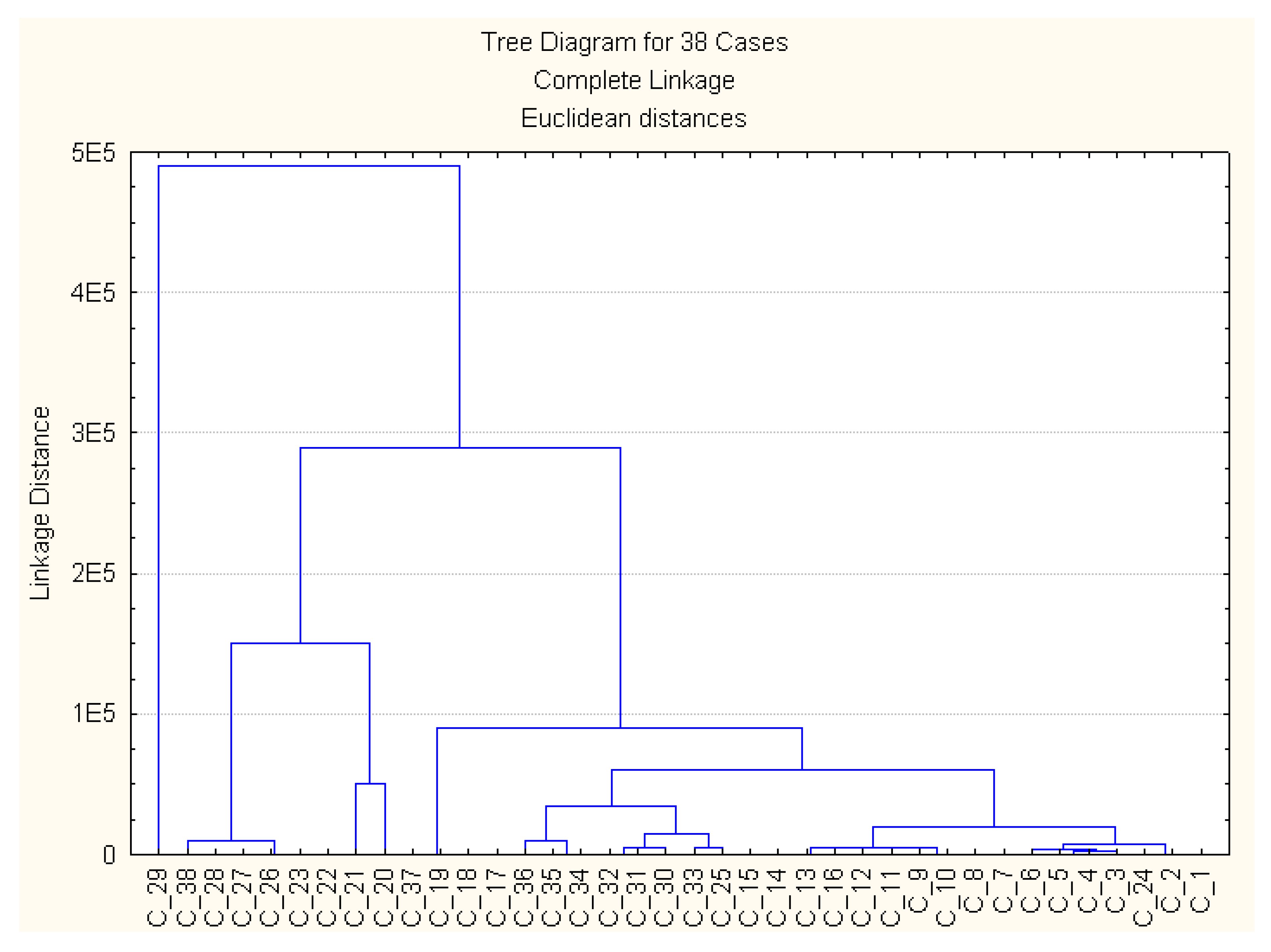
First, homogeneous groups of customers are formed according to two indicators determined by the first factor, selecting the variable “month” and “value”. Clustering is carried out in two stages - qualitative analysis using hierarchical methods and analysis using the k-means method. Exploration analysis to determine the possible number of groups is carried out using a hierarchical classification using different measures of similarity and differences in objects in groups—Euclidean distance, Manhattan distance, Chebyshev distance—to assess the degree of proximity of objects within groups and measures of distances between clusters—single, complete communication. By varying the distance measures, one can qualitatively evaluate the possible composition of clusters and the number of clusters. An analysis of the different partitions of the original sample by the method of hierarchical classification showed that it is possible to form three to six clusters, Figure 1.

For more reasonable objects grouping we take clustering methods that use quantitative criteria to assess the partition quality. These methods include the k-means method. Below the results of partitioning in which four groups (k = 4) and showing a significant difference between the classes formed among themselves are presented. The results of a single-factor analysis of variance to determine the similarity/difference groups are demonstrated in

Table 9. Results of single-factor analysis of variance.

Variable	The Intergroup Sum of Squares of Deviations for the Number of Degrees of Freedom Equal to 3	The Intragroup Sum of the Squares of Deviations for the Number of Degrees of Freedom Equal to 34	F-Test
Month	781,505.7	6325.706	14.0017
Value	489,827.5	4565.484	121.5945

.

The data was supplemented with information about the cluster to which the particular client belongs. Father for each cluster we calculate the basic descriptive statistics, build regression models and generate forecasts. The statistical characteristics (the mean, the standard deviation and the number of objects in each class) are shown in

Table 10. Descriptive statistics for selected clusters (k-means method).

Cluster	Number of Borrower’s	Borrower’s Numbers	Descriptive Statistics for the Variable Month		Descriptive Statistics for the Variable Value
			Mean	Standard Deviation	Mean	Standard Deviation
1	7	22, 23, 26–29, 38	33.4	15.44	327,142.9	76,313.9
2	6	17–21, 37	16	15.95	125,000	41,833.0
3	7	25, 31–36	51.4	13.35	52,142.9	11,495.3
4	18	1–16, 24, 30	14.6	12.26	22,222.2	8292.8

.

Since the number of clusters is not known in advance and the sample of clients is quite heterogeneous, to obtain a more justified partition into clusters, we use another machine learning method—Automated Neural Networks (ANN). Then we compare the effectiveness of two methods (algorithms) for obtaining client clusters—k-means method and Automated Neural Networks method.

To get the number of clusters we use the self-organizing map—a neural network with unsupervised learning. We divide the initial data into three subsamples. The first is the training sample in the amount of 70% of the total sample size, which is used to train the neural network and adjust its weights. The second subsample is a test sample, its volume is 15 percent, it is used to verify the correctness of training and retraining. The third subsample, a validated sample, serves to evaluate the accuracy of a neural network using “new data”. During the design of the adequate neural network, firstly, we set the topological dimension of the network by 5×5 neurons. As a simulation result, we have found that four classes of clients can be clearly distinguished since it is precisely four neurons that described the majority of the initial data.

The clustering results obtained using the ANN method is presented in

Table 11. Descriptive statistics for selected clusters (ANN method).

Cluster	Number of Borrower’s	Borrower’s Numbers	Descriptive Statistics for the Variable Month		Descriptive Statistics for the Variable Value
			Mean	Standard Deviation	Mean	Standard Deviation
1	7	22, 23, 26–29, 38	33.4	15.44	327,142.9	76,313.9
2	2	20, 21	6	0	175,000	35,355.3
3	11	17–19, 25, 31–37	40.4	20.9	69,545.5	25,734.7
4	18	1–16, 24, 30	14.6	12.26	22,222.2	8292.8

.

A comparative analysis of the clustering results (Table 10 and Table 11) demonstrates that the first and fourth clusters have the same composition of borrowers and the same values of all statistical indicators—mean, standard deviations, variation coefficient. Third clusters are similar in composition of borrowers, but the second clusters in the clustering based on the k-means method united six borrowers, and the ANN method combined only two. In addition, the variation coefficient of the indicator “value” in the third cluster of borrowers shows their significant heterogeneity when using the ANN method.

For a reasonable choice of one of the clustering methods and obtaining homogeneous groups of borrowers, we conduct an additional analysis of the robustness of the methods used for clustering. To do this, an additional binary variable is introduced into the initial data sample, reflecting borrower‘s problems with non-repayment of loans. Next, new clusters are formed taking into account this new factor. Clustering based on the k-means method showed the highest stability of clusters from the point of view of their identical composition before and after the addition of a new factor than clustering based on ANN. Therefore, to clustering clients and forming their homogeneous groups, the k-means method has been chosen.

At the next stage, the following information has been received: the number of the borrower’s clusters, cluster size, the share of working capital of each class in their total value, information about unit working capital. The most numerous cluster (18 borrowers) is the fourth characterized by the lowest credit values, from 10 to 35 thousand rubles, and the average credit fluctuation is quite high (37%). This cluster is rather unstable and determines about 10% of the total credit value, as shown in

Table 12. Summary information about clients’ clusters.

Indicator	The Value of the Indicator in the Cluster
	1	2	3	4
Number of objects in the cluster, people.	7	6	7	18
Total credit, rub.	2,290,000	750,000	365,000	400,000
Share of total credit,%	60.2	19.7	9.6	10.5
Minimum credit, rub.	290,000	100,000	40,000	10,000
Maximum credit, rub.	500,000	200,000	70,000	35,000
Average credit, rub.	327,143	125,000	52,143	22,222
Average credit period, months.	33.4	16	51.4	14.6
Standard deviation for credit, rub.	76,314	41,833	11,495	8293
Variation for credit	0.23	0.33	0.22	0.037

.

The third cluster is most congeneric as the variation is about 22%, the credit value is low—from 40 to 70 thousand rubles and about 9.6% of total credit sum, but the credit period for this cluster is largest—an average of 51.4 months. The second cluster includes few clients, has a high value of the average credit, can be characterized as a medium congeneric. The cluster which gives the highest income is the first, it is about 20% of all customers who take significant credits for a not very long time—on average 33 months, the cluster is stable.

Thus, based on machine learning methods—cluster analysis, factor analysis, and principal component method, the credit scoring model is proposed that allows assessing credit risks in homogeneous groups of borrowers for further decision-making about forming of differentiated requirements loan conditions for borrowers. For a deeper analysis of each customer’s cluster and for decision-making on credit policy, it is necessary to investigate statistics on the credit repayment. It is possible to design the regression model (for each cluster) of the credit repayment (in accordance with contractual obligations) from the variables of the credit value, credit period and other significant factors.

6. Conclusions

In the work, we have proved that under conditions of growing demand on credit resources in the Russian economy the importance of credit risks management system is strongly increased. Empirical studies have shown that credit risks are increased nonlinearly according to the main credit characteristics like credit risk level, credit terms, and credit interest rate. In the context of the active changing of the external and internal environment of Russian commercial banks, the engineering of the comprehensive knowledge about its activities and management of the credit portfolio quality using new approaches and tools has not only theoretical but also practical importance.

We have highlighted the problems of credit default risks increasing under the growing demand for credit resources. We have systematically analyzed approaches and methods aimed at reducing credit risks. It is shown that in order to reduce the credit portfolio risks banks need not only to apply the regulatory measures of the Bank of Russia but also to conduct thorough scoring of borrowers and the credit portfolio as a whole.

The new technology has been developed for quality management of the bank’s credit portfolio, which is based on the qualitative and quantitative indicators. The technology provides continuous scoring of the clients, allows clients classification by the homogeneity of credit histories, and provides support for management decisions on approving or rejecting a loan application in accordance with acceptable risk factors. To model the optimal structure of the credit portfolio according to the risk/return criterion for various values of the risk appetite of the decision-maker, a model of diversification of the loan portfolio has been proposed. The credit scoring model based on machine learning methods- cluster analysis, factor analysis, and principal component method has been supposed that allows assessing credit risks in homogeneous groups of borrowers. This model is the basis for decision-making on the formation of differentiated requirements for borrowers and loan conditions.