Article

The Development of a Defect Detection Model from the High-Resolution Images of a Sugarcane Plantation Using an Unmanned Aerial Vehicle

by
Bhoomin Tanut
and
Panomkhawn Riyamongkol
*
Computer Engineering Department, Faculty of Engineering, Naresuan University, Phitsanulok 65000, Thailand
*
Author to whom correspondence should be addressed.
Information 2020, 11(3), 136; https://doi.org/10.3390/info11030136
Submission received: 25 January 2020 / Revised: 22 February 2020 / Accepted: 26 February 2020 / Published: 28 February 2020
(This article belongs to the Special Issue UAVs for Smart Cities: Protocols, Applications, and Challenges)

Abstract

:
This article presents a defect detection model of sugarcane plantation images. The objective is to assess the defect areas occurring in the sugarcane plantation before the harvesting seasons. The defect areas in the sugarcane are usually caused by storms and weeds. This defect detection algorithm uses high-resolution sugarcane plantations and image processing techniques. The algorithm for defect detection consists of four processes: (1) data collection, (2) image preprocessing, (3) defect detection model creation, and (4) application program creation. For feature extraction, the researchers used image segmentation and convolution filtering by 13 masks together with mean and standard deviation. The feature extraction methods generated 26 features. The K-nearest neighbors algorithm was selected to develop a model for the classification of the sugarcane areas. The color selection method was also chosen to detect defect areas. The results show that the model can recognize and classify the characteristics of the objects in sugarcane plantation images with an accuracy of 96.75%. After the comparison with the expert surveyor’s assessment, the accurate relevance obtained was 92.95%. Therefore, the proposed model can be used as a tool to calculate the percentage of defect areas and solve the problem of evaluating errors of yields in the future.

Graphical Abstract

1. Introduction

Sugarcane is an economic crop of Thailand and the raw material of the sugar factory. Thailand has suitable geographical and climatic conditions for sugarcane cultivation. Moreover, it is the 4th largest sugar producer in the world after Brazil, India, and the European Union [1]. Currently, the Thai government supports the agriculture and biotechnology industry to improve the economy and increase the competitiveness of the country. The industry is operated by applying modern agricultural technology such as the use of sensor systems and advanced data analysis techniques [2]. The average age of sugarcane cultivation is 12 months per harvest. The assessment and survey of sugarcane plantation by the expert surveyor is operated in 2 stages: the first 4 months after planting, and the last 2 months before harvesting. For the harvesting methods, the sugarcane will be harvested by human labor and a sugar harvester [3].
Kamphaeng Phet province is one of the most widely cultivated sugarcane provinces in Thailand. It is located in the lower northern region of Thailand, with sandy soil suitable for farming and growing crops with an area of 2.1 million acres. The land use is divided into three groups: 1.24 million acres of agriculture, 0.47 million acres of forest, and 0.39 million acres of residential land. Kamphaeng Phet’s gross domestic product of 3547$ million is ranked 2nd in the northern region and ranked 4th in the country. The climatic condition in Kamphaeng Phet is categorized as tropical grassland with rain–drought alternation, and storms that cause damage to crops. The major economic crops of Kamphaeng Phet province in the farming sector include rice, cassava, corn, sugarcane, banana, and tobacco. Because the sugarcane can resist the intense storms more than other plants, it has the most cultivation area of 0.29 million acres [4].
Sugarcane assessment for the factory is one of the problems that has an impact on factory resource management such as labor, machinery, and production costs. Currently, the assessment of sugarcane yield before entering the factory depends on the assessment of expert surveyors. Surveyors use the individual’s personal assessment experience and it affects yield deviation [5]. In addition, there can be defects in the sugarcane plantation such as sugarcane falls due to storms and plants being stunted by weeds. The defect sugarcane areas cannot be detected by general survey, and it may influence deviation between assessment and actual yield. As mentioned above, the problem of error estimation leads to the development of the defect detection method for sugarcane plantations. Previous studies on the defect detection method uses two data sources: (1) satellite images and (2) unmanned aerial vehicle images. The data acquisition in both sources has different advantages and disadvantages. The details are as follows:
There are 24 high-definition satellites in Thailand which cover the areas with wide-angle images [6]. Thai Chot is one of the natural resource satellites used to capture the the areas covering the world, but there is an implication of high cost associated to access the specific plantation areas and a limitation to update the information. The disadvantage of using the satellite is that it takes 26 days/time to capture the images of the interesting areas and most of the areas would be covered by clouds [7].
An unmanned aerial vehicle (UAV) is an automatic airplane without a pilot on board [8]. High quality cameras are installed and equipped to take daylight and infrared photographs. The camera can record images from a long distance and broadcast them images to the controller. In addition, the recorded images have a high resolution in 4K, and it is suitable for image processing to analyze the health of agricultural plots.
An unmanned aerial vehicle was used to explore the space over the sugarcane plot to create a route map for cultivation [9]. Some researchers used a UAV to detect Bermuda grass in the sugarcane plots [10] and weeds in the sugar beet plantation [11]. A UAV was not only used to explore and analyze plant diseases in the vineyard [12] and sugarcane plots [13], but also classified the vegetation variety [14]. Moreover, there were studies which were conducted during the tilling stage of cultivation images for sugarcane yields assessment [15,16]. However, this research applied a UAV to assess sugarcane yields in the mature stage. As mentioned above, the defect in the sugarcane plantation needs to be analyzed for the sugarcane yield assessment. The proposed method uses the images from a UAV to analyze the damage rate of the defect areas. In addition, the defect rate from image processing techniques can be used to estimate the sugarcane yield together with climate factors.
The main contribution of this paper is to develop a framework to detect the defect areas in the sugarcane plantations. The sugarcane defect rate obtained from the study can be used to replace the climatic factors such as soil series and rainfall. In this research, the researchers have used fewer features to classify the sugarcane areas. The researchers in [16] have proposed eight statistical values (mean, average deviation, standard deviation, variance, kurtosis, skewness, maximum, and minimum) whereby the accuracy is low compared to the methods used in this proposed research which use mean and standard deviation with 13 filtering masks.
Moreover, in the future, the industrial plants will benefit in terms of resource management such as data collection, cost of climate factors survey, and reduction of yield deviation. The sugarcane industry can explore sugarcane plots faster. This will help to allocate the resources during the harvesting season in an efficient way, and consequently, the harvester machine can reduce the number of sugarcane burning. In Thailand, The burning of sugarcane is one cause of the air pollution problems (PM 2.5 or PM 10 ) by farmers during the harvesting season. As a result, when the factory uses the harvester machine, this can enhance the development of green industries in the future.

2. Material and Method

An unmanned aerial vehicle of the DJI company (Phantom4 model) was proposed for the collection of datasets to create a defect detection model. The DJI Phantom4 is capable of flying up to 30 min, with a wind resistance of 10 m/s and equipped with an ultra-high-definition quality camera which is 20,962 cm 2 calculated from 72 dpi. In this research, two software were proposed to develop the model, including (1) Google Earth Engine editor for creating coordinates of the sugarcane plantation, and (2) MATLAB 2015b for model development and image processing. The conceptual framework of the study is shown in Figure 1.
In Figure 1, the defect detection framework for sugarcane plantation consists of 4 main steps: data collection, image-preprocessing, defect detection model creation, and application program creation. The details of each steps are discussed below.

2.1. Data Collection

The sugarcane datasets were collected from a sugar factory in Kamphaeng Phet Province. After the data cleaning process, 2724 plots, out of the total 3442 plots, were left. The collection of data by unmanned aerial vehicles was done by random sampling considering different environmental factors, such as sugarcane varieties, sugarcane ratoon, soil series, and yield levels (Table 1).
The selection of patterns from the sample plantation was carried out by the Cartesian product method [17] from the factors in Table 1. The resulting Cartesian product had 594 patterns (3 × 3 × 3 × 22 = 594), in which only 90 data matched the pattern from the actual dataset. The details of the population (red spots) are shown in Figure 2A, and the samples (red spots) are shown in Figure 2B.
Figure 2B shows a sampling of the selected sugarcane plots in the province of Kamphaeng Phet. The sampling images were used to develop a model for analyzing the defect present in a sugarcane plantation. The sample datasets are shown in Figure 3.
A survey was done in September to October 2018 using the UAV, which consists of the four conditions: height from the ground at 200 m to 300 m, undefined environment, shooting time, and the size of the images (3078 × 5472 pixels). The images collected from the survey were used as the datasets for the study and development of the defect detection model.

2.2. Image Preprocessing

The image-preprocessing process is one of the crucial steps for the preparation of datasets before using image processing techniques. The images collected from the UAV have a shadow region formed during shooting at different times. The shadows were mostly created by trees and different sugarcane heights. Therefore, it is necessary to have shadow detection and shadow adjustment methods before the image is being processed. The sample image with the shadow region is shown in Figure 4.
The sugarcane area was divided into 2 categories: hard shadow and soft shadow [18]. The image was taken from a height of 200 m for both hard and soft shadow (Figure 4). The original image was converted to a grayscale and Otsu’s thresholding method was applied to detect the shadow region [19]. However, the sugarcane under the shadow region could not be analyzed as defects because of thresholding. Therefore, the shadow detection and the shadow adjustment were proposed before applying Otsu’s thresholding method.

2.2.1. Shadow Detection

Shadow detection is one of the methods in the image preprocessing step before applying the image processing technique. The shadow region affects the analysis of the defect areas in the image. Some researchers have suggested shadow detection of outdoor images [20] and infrared images [21]. In this study, a shadow detection algorithm using LAB [22] color space and statistical values [23] was proposed as shown in Figure 5.
The shadow detection method consists of the following steps.
  • Step 1: Convert the color image to LAB color space.
  • Step 2: Calculate the mean of each color plane followed by the standard deviation of L plane.
  • Step 3: Detect the shadow pixel by thresholding. The conditions for thresholding are shown in the Figure 5 and the algorithm is shown as a pseudo-code in Algorithm 1.
  • Step 4: Divide the areas into 2 regions: the shadow regions g i ( x , y ) and the non-shadow region regions h i ( x , y ) . The shadow region has a pixel value of 0 (black) and the non-shadow region has a pixel value of 255 (white). The results from the shadow detection method are used as an input for shadow adjustment process.
Algorithm 1 Pseudo-code description of a shadow detection. Input = UAV image. Output = Binary image
( g i ( x , y ) represents the shadow region and h i ( x , y ) represents the non-shadow region)
  1:   Procedure Shadow Detection (image)
  2:     height ← Image height from image
  3:     width ← Image width from image
  4:   vertical scan at h:
  5:   for x ϵ {0, height} do
  5:   raster scan at w:
  6:     for y ϵ {0, width} do
  7:       If mean (A (x ,y)) + mean (B (x,y)) <= 256
  8:          If (L (x ,y) <= mean (L)) – standard deviation (L) /3
  9:            shadow region ( g i ( x , y ) )
  10:          Else
  11:            non-shadow region ( h i ( x , y ) )
  12:          end if
  13:       Else
  14:          If pixel (L(x ,y)) < pixel(B (x ,y))
  15:            shadow region ( g i ( x , y ) )
  16:          Else
  17:            non-shadow region ( h i ( x , y ) )
  18:          end if
  19:       end if
  20:     end for
  21:   end for
  22:   End procedure

2.2.2. Shadow Adjustment

The shadow adjustment process was applied after the shadow detection process. Moreover, this process is considered as a crucial step for image preparation before entering the sugarcane image classification. Currently, there are a number of methods already developed for shadow adjustment methods, such as the shadow adjustment from RGB-D color images [24], the shadow adjustment of the high buildings from satellite images [25], and shadow adjustment for the survey of utilization areas [26]. The adjustment of a shadow depends on the amount of lights in shadows and non-shadow regions [27]. The flowchart of shadow adjustment method is shown in Figure 6.
The shadow adjustment process consists of 3 steps for calculating the light source of the shadow region g i ( x , y ) and the non-shadow region h i ( x , y ) areas. The constant ratio is calculated from the brightness values of the pixel in the shadow areas.
  • Step 1: Calculate the light source of the shadow and non-shadow areas in the output image given by the shadow detection method. The light source value was calculated from Equations (1) and (2).
    e 1 _ i = k _ i x = 1 M y = 1 N ( g i ( x , y ) ) p M N 1 / p
    where
    • e 1 _ i is the xy-summation of the shadow region.
    • M N is the number of pixels on the shadow region.
    • k _ i is the scale factor defined by R channel (KR), G channel (KG), B channel (KB).
    • p is the weight of each gray value in the light source.
    e 2 _ i = k _ i x = 1 M y = 1 N ( h i ( x , y ) ) p M N 1 / p
    where
    • e 2 _ i is the xy-summation of the non-shadow region.
    • M N is the number of pixels on the non-shadow region.
    • k _ i is the scale factor defined by R channel (KR), G channel (KG), B channel (KB).
    • p is the weight of each gray value in the light source.
  • Step 2: Determine the value of p that is suitable for adjusting the intensity of the shadow areas. Brightness, contrast, and average gradient of the shadow area were compared with the non-shadow areas. The appropriate p-values generated from the experiments is shown in Section 3.2.
  • Step 3: Calculate the constant ratio of the light source values in both areas and proceed to adjust the intensity of the shadow area as in Equation (3).
    g _ h i ( x , y ) = g i ( x , y ) · e 2 _ i / e 1 _ i
    where
    • g _ h i is the new shadow region.
    • e 2 _ i / e 1 _ i is the rate constant of shadow and non-shadow regions.
    • g i ( x , y ) is a shadow region.
After the shadow adjustment process, the shadow areas are usually brighter and sharper than original images. Therefore, those images were used for the development of the model for detecting the defects in the sugarcane plantation.

2.3. Defect Detection Model Creation

The development of the defect detection model in sugarcane plantation consists of 4 steps: (1) feature extraction, (2) classification of sugarcane areas, (3) defect area classification, and (4) data integration. The details are as follows.

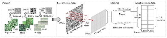
2.3.1. Feature Extraction

The feature extraction process is one of the essential steps for classification of objects within sugarcane plot such as sugarcane area, weeds, soil, water sources, roads, and trees. In this research, 90 UAV images were selected for texture analysis and image segmentation. For the image segmentation process, the image was resized to 3000 × 5000 pixels for non-border and non-missing parts of the sub-image. The researchers divided the image into 50 × 50 grid cells because the researcher can carefully label the images which are to be categorized. From 50 × 50 grid cells, 60,000 sub-images were generated from one image. However, the researchers selected a region of interest (50 × 50) from the image as the datasets as shown in Table 2, for training the model.
The datasets were divided into two categories as shown in Table 2: Dataset 1 consists of sugarcane, trees, and weeds images whereas dataset 2 contains weeds and trees images. In both of the datasets, 80–20 ratio was used to split the datasets into training and testing sets. Each category of datasets has 5 varying sizes such as (1) 10 × 10, (2) 20 × 20, (3) 25 × 25, (4) 40 × 40, and (5) 50 ×50, respectively, as shown in Table 4. This size is calculated using the greatest common factor (GCF) algorithm. The conceptual framework of feature extraction is presented in Figure 7.
The conceptual framework is explained by using 50 × 50 pixel which consists of 4 steps:
  • Step 1: Convert RGB color image to grayscale format.
  • Step 2: Convolute the grayscale images by 13 filtering masks to get the features. In this research, standardized filters [28] (3 × 3) as shown in Figure 8 was used.
  • Step 3: The statistical values such as mean and standard deviation are calculated from step 2. This process achieves 26 characteristics.
  • Step 4: Select the features that are related to the class of the category using the WEKA program [29]. WEKA program uses the “Information Gain-Based Feature” selection method to find the significant features which is known as entropy. The features must pass the threshold value of more than 0.05. This value is selected using a T-score distribution method which separates the group of data obtained from entropy and eliminates those groups that have least relationship with the class (sugarcane, trees, and weeds). When the threshold value 0.05 was used as a condition, it gives the most significant features for the classification of sugarcane areas.

2.3.2. The Sugarcane Areas Classification Process

The sugarcane area classification is a process used to classify sub-areas (sugarcane, trees, and weed) within an image. The dataset used in the development of the process is shown in Table 2; which consists of training and validation sets for training purposes and the testing set to evaluate the model. In the experiments, the K-nearest neighbors method [30] was selected to develop a model for classification of sugarcane areas.

2.3.3. The Defect Areas Classification Process

This process was carried out after identification of sugarcane areas from the previous step. In this process, color analysis and color selection methods were used to eliminate other colors except green shades. The color selection method is performed by converting the RGB color image into the HSV color space and then selecting Hue channel into 3 ranges (yellow–green: 60–80 degrees, green: 81–140 degrees, and green–cyan: 141–169 degrees) of green shades [31]. The color selection process provides only the areas of trees, weeds, and green water sources. However, the stunted weeds, ground, and roads were eliminated since their color space does not fall under the given range.

2.3.4. Data Integration Process

The data integration is a process that combines the results of the sugarcane areas classification and defect areas classification. This process is performed by the logical AND operator to integrate the defects and sugarcane areas.

2.4. Application Program Creation

The graphical user interface (GUI) was developed to assist the selection of sugarcane areas from the images. Moreover, the user interface can be used to draw the polygonal lines [32] to select the region of interest and help to reduce errors by avoiding other objects in the image. After drawing a polygon into the desired area, the program will analyze the selected area and identify the faulty spots such as water sources, weeds, defect sugarcane, etc. The defect detection rate in the GUI is shown as a percentage in the top right corner of the program window as shown in Figure 17.

3. Experiment Results

The aim of developing a defect detection model in sugarcane plantation images is to reduce the yield estimation error. The model uses high-resolution images captured from the UAV. The proposed methods consists of 4 steps: data collection, image-preprocessing, defect detection model creation, and application program creation. For image preprocessing, the researchers designed two experiments: (1) performance testing for shadow detection and (2) the performance testing for shadow adjustment. Whereas, for the evaluation of defect detection models, the performance testing for sugarcane area classification and defect area classification experiments were designed.

3.1. The Performance Testing for Shadow Detection

The shadow detection is one of the image preprocessing steps. The experiment was carried out with experts by manually plotting shadow and non-shadow areas as shown in Figure 9A. The sugarcane plot contains 100 by 100 grid cells. The conditions for identification of the shadow region in the grid cell for both expert and proposed model must have 50% of shadow in the square (thick square) [33]. The example of experiments for shadow detection is shown in Figure 9.
The experiment was conducted to compare the results of all 90 images. The experimental results found that the average precision was 75.92% with a recall of 92.23% and F1-measure of 80.11%. The overall accuracy obtained from the experiments was 98.44%. The relationship between the sensitivity (true positive rate: TP) and 1-specificity rate (false positive rate: FP) is shown in Figure 10.
The ROC curve of the experimental result shows that the average sensitivity and 1-specificity was 85.80% and 99.88% respectively. The result has a high performance due to the adjacent left corner and the average areas under the curve (AUC) which was 99.67%. Therefore, the method proposed for shadow detection areas is highly effective in detecting the shadow region in the sugarcane areas.

3.2. The Performance Testing for Shadow Adjustment

The results obtained from shadow detection method is passed as an input to this method. This process adjusts the intensity of the shadow areas from approaching the non-shadow areas. In this method, the parameter p of the Minkowski norm [34] (Equations (2) and (3)) is adjusted from 1 to 10 to get the proper p-value. The p-value is selected based on 3 factors such as brightness, contrast, and the average gradient of each image. The sample p-value for one of the sugarcane plant images is shown in Table 3.
This process selects the result that is closest to the value of the non-shadow areas from all three factors in each color plane. The experimental results are shown in Figure 11.
The experiment found that most of the images have an exponential value of p = 1, but there are some images with p-value of 2, 3, and 4, due to brighter non-shadow region than the shadow region. As a result, it is necessary to adjust the p-value to be closest to the non-shadow area.

3.3. The Performance Testing for Sugarcane Areas Classification

The sugarcane areas classification is a process to identify the categories of objects present in the images such as sugarcane, trees, weeds, and others. The experiment is divided into 2 parts: (1) the experiment for feature selection and (2) the experiment to develop model for sugarcane area classification. The experiment was conducted with 2 datasets as shown in Table 2.

3.3.1. The Experiment of Feature Selection

Feature selection is a process of gathering important attributes from the image which can help to distinguish from the other image. The selection of features is carried out by correlation with classes of each category from the sub-images of the 2 datasets. The features that passed the threshold value of 0.05 were used to train the model and eliminate the less important features. The experimental results are shown in Table 4.
In Table 4, the features that do not satisfy the given conditions are underlined and the other features were used in training the model.

3.3.2. The Experiment of Sugarcane Area Classification Model Creation

For sugarcane classification, 2 datasets were used to train the model using the K-nearest neighbor algorithm. After training the model, the model which gives the best accuracy to classify the sugarcane area was selected for the research. The model was trained and validated using the 10-fold cross-validation method. The experimental results are shown in Table 5.
The experiment shows that dataset 1 with size 50 × 50 pixels obtained the highest accuracy of 91.38% with the 10-fold cross-validation whereas, the testing set gave of 85.65% which results in overfitting. Dataset 2 with a size 50 × 50 pixels had the highest accuracy of 96.75% with a 10-fold cross-whereas, the testing set gave 95.01%. Therefore, the dataset 2 was proposed for the development of sugarcane area classification model but both of the datasets could not identify trees. The results given by the experiments were compared with what the sugarcane surveyor experts marked. The only condition for identification of sugarcane area by the experts and models that there must be more than 50% of sugarcane area in the grid cell. Figure 12 shows the sugarcane classification done by the model and the experts.
In Figure 12, the non-sugarcane areas are identified by thick squares. In the performance testing of model 1 (created from dataset 1): the expert identified the trees, weeds, and other areas that are non-sugarcane for comparison with the result of the model. However, in model 2 (created by dataset 2): the expert identified the weeds and other areas that are non-sugarcane for comparison with the result of model. The results obtained from classification of sugarcane areas by experts and the proposed model are shown in Table 6.
The relationship between sensitivity (true positive rate: TP) and 1-specificity (false positive rate: FP) calculated from confusion metrics is shown in Figure 13.
The ROC curve of experiment result found that model 2 is more efficient than model 1. The average sensitivity in the model 2 was 74.03%, and the 1-specificity was 87.54%. The curve of model 2 was adjacent to the left corner and the average areas under curve (AUC) was 92.27% (see Figure 13B). The average sensitivity in the model 1 69.38%, and the 1-specificity was 71.01%. The average areas under curve (AUC) was 89.42% (see Figure 13A). Both models cannot identify the trees in sugarcane plantation images. Therefore, model 2 is chosen to create a model for sugarcane area classification.

3.4. The Performance Testing for Defect Areas Classification

The sugarcane defect area classification is a process applied after the shadow detection, the shadow adjustment, and the sugarcane area classification process. This experiment consists of results from the color selection and the data integration. The experiment was compared with what the sugarcane surveyor experts marked to identify the defect areas that were divided into 100x100 grid cells in the original images. The only condition for identification of the defect area by experts and the models is that there must be more than 50% of defects (thick square) in the square. See an example of the operation in Figure 14.
The experiment was conducted to compare the results of all 90 images. The experiment results found that the average precision was 76.06% with recall value of 81.49% and F1-measure 79.73%. The overall accuracy of defect areas was 87.20%. The relationship between sensitivity (true positive rate: TP) and 1-specificity (false positive rate: FP) is shown in Figure 15.
This ROC curve of experiment result found that the average sensitivity and 1-specificity was 87.20% and 75.78% respectively. The result has a high performance due to the adjacent left corner and the average areas under curve (AUC) was 92.95%. Therefore, the parameters and the model can be applied for application program creation.

4. Result and Discussion

The defect detection model was developed by image processing techniques with high-resolution images taken from an unmanned aerial vehicle. The model consists of five main processes such as shadow detection, shadow adjustment, feature extraction, sugarcane area classification, and defect area classification process. The results obtained from the experiments were used to develop the application to assess the defect on the sugarcane plantation. The results of the defect detection model is shown in Figure 16.
The image preprocessing techniques consists of the shadow area detection and shadow adjustment process. The experiment found that the shadow detection method can detect the shadow cast by trees and high sugarcane with the accuracy of 99.67% as shown in Figure 16B. The shadow adjustment process applies intensity adjustment in the shadow areas as a result shown in Figure 16C.
In the sugarcane area classification, 50 × 50 pixels sub-images were used for extraction of features for the development of model. After training the features, dataset 2 (having sugarcane and weeds) gave the highest accuracy in the development of the model. However, the sugarcane area classification model could not identify the trees in either of the datasets, but it could identify the sugarcane area and weeds with the accuracy 92.27% for ROC curve in Figure 13B. The result of the sugarcane area classification is shown in Figure 16D.
The defect detection, the color selection process (see in Figure 16E) and data integration process were proposed. The data integration process was operated by combining the results of sugarcane area classification and color selection process (see in Figure 16F). The experiment found that the defect detection process was able to identify the defect in sugarcane plantation image with the accuracy 92.95%.
The overall experiment of the proposed method can detect the defects such as water sources, defect areas, ground, residences, and road in the sugarcane plantation. However, the method could not identify trees in sugarcane plantation. Therefore, the researcher developed the graphical user interface (GUI) to solve the problem of identifying trees in the sugarcane plantation while drawing the polygon on the interested areas. The GUI is shown in Figure 17.
The GUI is used for drawing the interesting regions for classifying the sugarcane areas whereby the trees in the image are not selected. The example plantation (10008002) as given in Figure 17, which shows the percentage of the defects in interested areas. With the introduction of the GUI, the experts are satisfied with the program with a satisfaction level of good (4.53).The performance comparisons of the proposed methods with the methods discussed in the literature review is presented in Table 7. The description presented on for table is reflected as per the information given in the reference paper.
The proposed method is different from the methods discussed in the literature. The researchers in [10,12,13] have analyzed the sugarcane plants in the mature stage, the same as the proposed method. However, different features and classifiers were used resulting in different accuracy. When comparing our results with the other methods, the proposed classifier generated an overall accuracy of 96.75% which is higher than the other methods that use the plants in the mature stage. The higher accuracy is due to the introduction of shadow detection and shadow adjustment preprocessing steps. In our approach, the researchers have extracted features using standard deviation, mean value, and 13 filtering masks. The researchers have not used other statistical values such as kurtosis, skewness, variance, etc. because it generated 82% [16] accuracy which is less than the proposed methods. The other methods were not compared since the detection is done during the tilling stage.

5. Conclusions

For the development of the model to analyze the defect areas of the sugarcane plantations, high-resolution image taken from an unmanned aerial vehicle was used. This model uses shadow detection, shadow adjustment, feature extraction, and classification methods. For feature extraction, the algorithm was developed by using 13 filter masks together with convolution operations into the sub-images. In each mask, the mean and standard deviation were calculated which makes up to 26 characteristics. The result of the process obtained 26 characteristics from the mean and standard deviation of the data to represent the value of the sub-image. The feature selection method was used based on the calculation of entropy between attributes and the class labeling. The 22 features extracted from the feature selection methods were trained and tested using the K-nearest neighbors classification algorithm in WEKA. The algorithm provided an accuracy of 96.75%. The model can classify the objects in the image, including water sources, defect areas, ground, residences, and roads precisely, but it cannot classify trees. Some parts of the trees and sugarcane have similar characteristics when extracted, thus making it difficult to distinguish between the sugarcane and trees. However, this method can be applied in conjunction with the selection of areas, excluding trees from the image. Therefore, while selecting the sugarcane plot on the GUI application, the user must avoid trees in order to have a high accuracy of sugarcane detection areas. The developed model can be used as a tool to calculate the percentage of defect areas, which can possibly solve the problem on sugarcane yield deviation. For future work, an automatic method such as Fourier analysis can be applied for detecting the tree automatically and the model will be improved to classify the objects with greater accuracy. Moreover, the industrial plants will benefit in resource management such as data collection, cost of climate factors survey, and yield deviation reduction.

Author Contributions

Conceptualization, B.T. and P.R.; methodology, B.T.; software, B.T.; validation, B.T. and P.R.; formal analysis, B.T.; investigation, P.R.; resources, B.T.; data curation, B.T.; writing–original draft preparation, B.T. and P.R.; writing–review and editing, B.T. and P.R.; visualization, B.T.; supervision, P.R.; project administration, B.T. and P.R.; funding acquisition, B.T. and P.R. All authors have read and agreed to the published version of the manuscript.

Funding

This research received no external funding.

Acknowledgments

We thank the Nakornphet Sugar Co. Ltd. and the VISION LAB of Naresuan University for their kind cooperation in this project.

Conflicts of Interest

The authors declare no conflict of interest.

References

  1. Sahu, O. Assessment of Sugarcane Industry: Suitability for Production, Consumption, and Utilization. Ann. Agrar. Sci. 2018, 16, 389–395. [Google Scholar] [CrossRef]
  2. Office, Eastern Region Development Commission. Targeted Industries. Available online: https://www.eeco.or.th/en/content/targeted-industries (accessed on 1 December 2019).
  3. Terpitakpong, J. Sustainable Sugarcane Farm Management Guide; Sugarcane and Sugar Industry Information Group, Office of the Cane and Sugar Board Ministry of Industry: Bangkok, Thailand, 2017; pp. 8–15. [Google Scholar]
  4. Nopakhun, C.; Chocipanyo, D. Academic Leadership Strategies of Kamphaeng Phet Rajabhat University for 2018–2022 Year. Golden Teak Hum. Soc. Sci. J. (GTHJ) 2019, 25, 35–48. [Google Scholar]
  5. Panitphichetwong. Bundit, 24 June 2017.
  6. Geo-Informatics. The Information Office of Space Technology and Remote Sensing System. Geo-Informatics and Space Technology Office. Available online: https://gistda.or.th/main/th/node/976 (accessed on 19 June 2019).
  7. Yano, I. Weed Identification in Sugarcane Plantation through Images Taken from Remotely Piloted Aircraft (Rpa) and Knn Classifier. J. Food Nutr. Sci. 2017, 5, 211. [Google Scholar]
  8. Plants, Institute for Surveying and Monitoring for Planting of Narcotic. Knowledge Management of Unmanned Aircraft for Drug Trafficking Surveys. Office of the Narcotics Control Board. Available online: https://www.oncb.go.th/ncsmi/doc3/ (accessed on 19 June 2019).
  9. Luna, I. Mapping Crop Planting Quality in Sugarcane from Uav Imagery: A Pilot Study in Nicaragua. J. Remote Sens. 2016, 8, 50. [Google Scholar] [CrossRef] [Green Version]
  10. Girolamo-Neto, C.D.; Sanches, I.D.; Neves, A.K.; Prudente, V.H.; Körting, T.S.; Picoli, M.C. Assessment of Texture Features for Bermudagrass (Cynodon Dactylon) Detection in Sugarcane Plantations. Drones 2019, 3, 36. [Google Scholar] [CrossRef] [Green Version]
  11. Mink, R.; Dutta, A.; Peteinatos, G.G.; Sökefeld, M.; Engels, J.J.; Hahn, M.; Gerhards, R. Multi-Temporal Site-Specific Weed Control of Cirsium arvense (L.) Scop. And Rumex crispus L. in Maize and Sugar Beet Using Unmanned Aerial Vehicle Based Mapping. Agriculture 2018, 8, 65. [Google Scholar] [CrossRef] [Green Version]
  12. Matese, A.; Di Gennaro, S.F. Practical Applications of a Multisensor Uav Platform Based on Multispectral, Thermal and Rgb High Resolution Images in Precision Viticulture. Agriculture 2018, 8, 116. [Google Scholar] [CrossRef] [Green Version]
  13. Kumar, S.; Mishra, S.; Khanna, P. Precision Sugarcane Monitoring Using Svm Classifier. Procedia Comput. Sci. 2017, 122, 881–887. [Google Scholar] [CrossRef]
  14. Liu, B.; Shi, Y.; Duan, Y.; Wu, W. Uav-Based Crops Classification with Joint Features from Orthoimage and DSM Data. ISPRS Int. Arch. Photogramm. Remote Sens. Spat. Inf. Sci. 2018, 42, 1023–1028. [Google Scholar]
  15. Sanches, G.M.; Duft, D.G.; Kölln, O.T.; Luciano, A.C.; De Castro, S.G.; Okuno, F.M.; Franco, H.C. The Potential for Rgb Images Obtained Using Unmanned Aerial Vehicle to Assess and Predict Yield in Sugarcane Fields. Int. J. Remote Sens. 2018, 39, 5402–5414. [Google Scholar] [CrossRef]
  16. Yano, I.H.; Alves, J.R.; Santiago, W.E.; Mederos, B.J. Identification of Weeds in Sugarcane Fields through Images Taken by Uav and Random Forest Classifier. IFAC-PapersOnLine 2016, 49, 415–420. [Google Scholar] [CrossRef]
  17. Oooka, K.; Oguchi, T. Estimation of Synchronization Patterns of Chaotic Systems in Cartesian Product Networks with Delay Couplings. Int. J. Bifurc. Chaos 2016, 26, 1630028. [Google Scholar] [CrossRef]
  18. Natarajan, R.; Subramanian, J.; Papageorgiou, E.I. Hybrid Learning of Fuzzy Cognitive Maps for Sugarcane Yield Classification. Comput. Electron. Agric. 2016, 127, 147–157. [Google Scholar] [CrossRef]
  19. Anoopa, S.; Dhanya, V.; Kizhakkethottam, J.J. Shadow Detection and Removal Using Tri-Class Based Thresholding and Shadow Matting Technique. Procedia Technol. 2016, 24, 1358–1365. [Google Scholar] [CrossRef] [Green Version]
  20. Hiary, H.; Zaghloul, R.; Al-Zoubi, M.D. Single-Image Shadow Detection Using Quaternion Cues. Comput. J. 2018, 61, 459–468. [Google Scholar] [CrossRef]
  21. Park, K.H.; Kim, J.H.; Kim, Y.H. Shadow Detection Using Chromaticity and Entropy in Colour Image. Int. J. Inf. Technol. Manag. 2018, 17, 44. [Google Scholar] [CrossRef]
  22. Chavolla, E.; Zaldivar, D.; Cuevas, E.; Perez, M.A. Color Spaces Advantages and Disadvantages in Image Color Clustering Segmentation; Springer: Cham, Switzerland, 2018; pp. 3–22. [Google Scholar]
  23. Suny, A.H.; Mithila, N.H. A Shadow Detection and Removal from a Single Image Using Lab Color Space. Int. J. Comput. Sci. Issues 2013, 10, 270. [Google Scholar]
  24. Xiao, Y.; Tsougenis, E.; Tang, C.K. Shadow Removal from Single Rgb-D Images. In Proceedings of the IEEE Conference on Computer Vision and Pattern Recognition 2014, Columbus, OH, USA, 23–28 June 2014. [Google Scholar]
  25. Shahtahmassebi, A.; Yang, N.; Wang, K.; Moore, N.; Shen, Z. Review of Shadow Detection and De-Shadowing Methods in Remote Sensing. Chin. Geogr. Sci. 2013, 23, 403–420. [Google Scholar] [CrossRef] [Green Version]
  26. Movia, A.; Beinat, A.; Crosilla, F. Shadow Detection and Removal in Rgb Vhr Images for Land Use Unsupervised Classification. ISPRS J. Photogram. Remote Sens. 2016, 119, 485–495. [Google Scholar] [CrossRef]
  27. Ye, Q.; Xie, H.; Xu, Q. Removing Shadows from High-Resolution Urban Aerial Images Based on Color Constancy. Int. Arch. Photogramm. Remote Sens. Spatial Inf. Sci. 2012, 39, 525–530. [Google Scholar] [CrossRef] [Green Version]
  28. Gonzalez, R.C.; Faisal, Z. Digital Image Processing, 2nd ed.; CRC Press: Boca Raton, FL, USA, 2019. [Google Scholar]
  29. Janošcová, R. Mining Big Data in Weka; School of Management in Trenčín: Trenčín, Slovakia, 2016. [Google Scholar]
  30. Imandoust, S.B.; Bolandraftar, M. Application of K-Nearest Neighbor (Knn) Approach for Predicting Economic Events Theoretical Background. Int. J. Eng. Res. Appl. 2013, 3, 605–610. [Google Scholar]
  31. WorkWithColor.com. The Color Wheel. Available online: http://www.workwithcolor.com/the-color-wheel-0666.htm (accessed on 10 December 2019).
  32. Zunic, J.; Rosin, P.L. Measuring Shapes with Desired Convex Polygons. IEEE Trans. Pattern Anal. Mach. Intell. 2019. [Google Scholar] [CrossRef] [PubMed] [Green Version]
  33. Shen, J.; Zhang, C.J.; Jiang, B.; Chen, J.; Song, J.; Liu, Z.; He, Z.; Wong, S.Y.; Fang, P.H.; Ming, W.K. Artificial Intelligence versus Clinicians in Disease Diagnosis: Systematic Review. JMIR Med. Inform. 2019, 7, e10010. [Google Scholar] [CrossRef] [PubMed] [Green Version]
  34. Cipolla, R.; Battiato, S.; Farinella, G.M. (Eds.) Registration and Recognition in Images and Videos; Springer: Berlin, Germany, 2014; Volume 532, pp. 38–39. [Google Scholar]
Figure 1. The conceptual framework of the defect detection model.
Information 11 00136 g001
Figure 2. Population and sampling data of sugarcane plantation: (A) population and (B) sampling.
Information 11 00136 g002
Figure 3. The data collection of the sugarcane plantation sampling.
Information 11 00136 g003
Figure 4. The top view of the sugarcane plantation image captured by the unmanned aerial vehicle (UAV).
Information 11 00136 g004
Figure 5. Shadow detection algorithm.
Information 11 00136 g005
Figure 6. Overview of shadow adjustment.
Information 11 00136 g006
Figure 7. The conceptual framework of feature extraction.
Information 11 00136 g007
Figure 8. The characteristics of 13 filtering masks.
Information 11 00136 g008
Figure 9. The comparison results between experts and the shadow detection process. (A,C) Original image, (B) the results of the expert, and (D) the results of the shadow detection.
Information 11 00136 g009
Figure 10. ROC curve results of the shadow detection process.
Information 11 00136 g010
Figure 11. The experimental result of adjusting the variable p of the image dataset.
Information 11 00136 g011
Figure 12. The comparison between experts and the sugarcane area classification model. (A) The results from expert of dataset 1, (B) the results from model of dataset 1, (C) the results from expert of dataset 2, and (D) the results from model of dataset 2.
Information 11 00136 g012
Figure 13. ROC curve results of the sugarcane area classification model. (A) ROC curve results of model 1 and (B) ROC curve results of model 2.
Information 11 00136 g013
Figure 14. Comparison results between experts and the defect defection model. (A) The results of the expert and (B) the results of the defect defection model.
Information 11 00136 g014
Figure 15. ROC curve results of the defect detection model.
Information 11 00136 g015
Figure 16. The result of the defect detection model. (A) Original image, (B) the result of shadow detection, (C) the result of shadow adjustment, (D) the result of sugarcane area classification, (E) the result of color selection, and (F) the result of defect area classification.
Information 11 00136 g016
Figure 17. The result of defect detection process together with the graphical user interface.
Information 11 00136 g017
Table 1. Environmental factors of sugarcane plantation in 2017.
FactorDetails of the Factors
VarietiesLK-91-11, Khon Kaen 3, U Thong 11
RatoonRatoon 1, Ratoon 2, Ratoon 3
Soil series3, 4, 5, 6, 7, 15, 17, 18, 21, 22, 23, 33, 35, 36, 38, 40, 44, 46, 48, 49, 55, 56
Yield levelsLow, Medium, High
Table 2. The dataset used for feature extraction and training the model.
CategoryDataset 1Dataset 2
Training and Validation SetTesting SetTraining and Validation SetTesting Set
Sugarcanes5956144959561449
Trees2820705--
weed31447863144786
Total11,890294091002235
Table 3. The example experiment of the shadow adjustment process.
Region and p/ConditionBrightnessContrastAverage Gradients
rgbrgbrgb
shadow region46.6067.5463.8221.6322.6221.023.293.853.52
p = 1130.28146.91126.1652.5346.0545.4377.3377.2574.22
p = 2130.05146.84126.2752.4546.0345.4777.1677.2074.30
p = 3129.87146.76126.3152.3946.0045.5077.0277.1474.35
p = 4129.74146.69126.3652.3545.9945.5076.9277.1074.35
p = 5129.66146.64126.3952.3245.9745.5276.8577.0774.38
p = 6129.59146.60126.4252.3045.9645.5376.8077.0474.40
p = 7129.55146.57126.4552.2945.9645.5476.7677.0274.42
p = 8129.51146.55126.4852.2845.9545.5576.7477.0174.43
p = 9129.48146.54126.5052.2745.9545.5576.7177.0074.45
p = 10129.46146.53126.5252.2645.9545.5676.6976.9974.46
non shadow region130.32146.92126.1551.8945.7545.7171.4573.1770.84
Table 4. Feature selection data for all sub-images.
AttributeDataset 1Dataset 2
10 × 1020 × 2025 × 2540 × 4050 × 5010 × 1020 × 2025 × 2540 × 4050 × 50
Mean10.0270.0470.0560.0740.0830.0260.0380.0450.0610.070
Mean20.0330.0550.0660.0850.1000.0300.0460.0550.0680.077
Mean30.0560.0840.0900.1150.1230.0480.0640.0720.0850.096
Mean40.0570.0870.0990.1200.1270.0490.0670.0760.0940.102
Mean50.0680.1030.1160.1380.1450.0570.0810.0930.1040.115
Mean60.0680.1040.1150.1370.1460.0570.0840.0940.1060.117
Mean70.0650.1070.1210.1490.1560.0550.0880.0990.1170.124
Mean80.0690.1080.1220.1480.1600.0570.0880.0990.1180.126
Mean90.0480.0760.0860.1050.1200.0410.0630.0680.0820.093
Mean100.0540.0290.0190.0050.0040.0800.0560.0410.0170.014
Mean110.0480.0200.0150.0080.0110.0740.0370.0300.0230.025
Mean120.0580.0230.0130.0050.0080.0940.0590.0470.0280.023
Mean130.0460.0170.0090.0050.0080.0760.0380.0300.0140.018
Std10.0900.2240.2950.4650.5190.0120.1080.1760.3710.458
Std20.0990.2620.3400.4970.5480.0160.1480.2280.4300.513
Std30.0960.1870.2350.3630.4190.0110.0620.1050.2390.309
Std40.1160.2380.2950.4320.4810.0230.1130.1730.3320.402
Std50.1750.3290.3980.5340.5700.0650.2030.2840.4570.522
Std60.1470.2640.3250.4690.5210.0400.1320.1920.3600.438
Std70.3190.5030.5510.6070.6110.2490.4860.5600.6690.690
Std80.1970.3630.4310.5590.5920.0900.2520.3370.5130.571
Std90.1000.2420.3100.4790.5330.0180.1130.1820.3810.466
Std100.1000.2210.2870.4480.5040.0170.0960.1580.3480.438
Std110.0950.2270.2960.4680.5330.0130.1080.1760.3910.491
Std120.1050.2550.3320.5070.5660.0210.1380.2190.4450.536
Std130.1050.2310.3000.4720.5330.0250.1110.1820.3940.492
Table 5. Performance of the K-nearest neighbors algorithm, K = 31.
Sub-Image Size/DatasetDataset 1Dataset 2Average
10-Fold Cross-ValidationTesting Set10-Fold Cross-ValidationTesting SetAccuracy
10 × 1081.494577.904387.494586.158683.2629
20 × 2086.694682.792192.846291.546288.4697
25 × 2588.523583.361294.318792.422389.6564
40 × 4090.511785.470496.065994.612491.6651
50 × 5091.384285.652296.747395.010992.1986
Table 6. Tabulation of precision, recall, f1-measure, and accuracy of each dataset.
Performance FactorsDataset 1Dataset 2
Precision67.44%77.58%
Recall70.19%80.79%
F1-measure66.67%77.53%
Overall accuracy69.38%85.66%
Table 7. Comparison of weed detection applications considering factors such as overall accuracy (OA), classifier, and types of features used.
CropStageDetectionOAClassifierFeature Used
Sugarcane [10]matureweed92.54%RFMultispectral
VI
Texture
Sugar beet [11]tilleringweed96%CHMMultispectral
VI
Maize [11]tilleringweed80%CHMMultispectral
VI
Vineyard [12]matureMissing plant80%CWSIMultispectral
NDVI
Sugarcane [13]matureLeaf Disease96%SVMSpectral
Sensor Data
Sugarcane [15]tilleringSugarcane Stalk--Spectral
GRVI
Sugarcane [16]tilleringweed82%RFSpectral
Texture
Statistical
Mean
Average Deviation
Standard Deviation
Variance
Kurtosis
Skewness
Maximum
Minimum
Sugarcanematureweed96.75%KNNSpectral
This paper Texture
Mean
Standard deviation
SVM: Support Vector Machine; RF: Random Forest; KNN: K-Nearest Neighbors; CHM: Canopy Height Model; VI: Vegetation Index; NDVI: Normalized Difference Vegetation Index; GRVI: Green-Red Vegetation Index.

