Abstract
Energy consumption is a relevant matter in the design of IoT applications. Edge units—sensors and actuators—save energy by operating intermittently. When idle, they suspend their operation, losing the content of the onboard memory. Their internal state, needed to resume their work, is recorded on external storage: in the end, their internal operation is stateless. The backend infrastructure does not follow the same design principle: concentrators, routers, and servers are always-on devices that frustrate the energy-saving operation of edge devices. In this paper, we show how serverless functions, asynchronously invoked by the stateless edge devices, are an energy-saving option. We introduce a basic model for system operation and energy footprint evaluation. To demonstrate its soundness, we study a simple use case, from the design to a prototype.
1. Introduction
A Internet of Things (IoT) system consists of a spatially distributed network of autonomous, computationally constrained edge devices: the sensors and the actuators. They produce data that a networking infrastructure delivers to backend servers. Using the computing power available on servers, such an architecture can process a large amount of data. In principle, the control system should optimize system efficiency, including energy consumption [1]. However, it has an energy footprint that the designer cannot overlook.
For instance, the purpose of the fog approach is to make more efficient and reactive the operation of the backend infrastructure. For this, it introduces layers of intermediate devices that provide the edge of a proxy interface to the servers. However, in that way, the overall energy consumption grows. If we consider the operational style of fog components, we observe that they need to be permanently operational, so that their energy consumption depends only marginally on load. Instead, an energy-wise practice is to avoid power consumption during idle periods. Therefore, we understand that, when considering the energy footprint of a IoT system, we need to take into account all components, including the backend control system. In summary, fog and edge computing have superior performance, but they do not help to make a greener IoT.
Examining the edge of an IoT system, we observe that power-saving techniques are in place and widely used for sensors and actuators. There are strong motivations for this, as such devices are often battery-operated, or harvest power from the environment. The technique to reduce energy consumption consists of the sporadic activation of the sensor, which spends most of the time in standby with negligible power consumption.
Various suspend modes exist for edge units: from the de-activation of the wireless transceiver to the timed shutdown of the whole device. In the latter case, only a timer runs to reboot the device after a defined time, thus reducing the energy consumption of orders of magnitude. However, when the device enters such standby mode, it loses the internal state: to some extent, its operation is stateless.
As a general rule, IoT applications require a stateful operation. Therefore, if not in edge units, the state of the system must be recorded elsewhere: either in onboard hardware, consuming precious energy, or in the backend infrastructure. For instance, the reference time may be retrieved after each reboot from a time server, instead of using the internal clock. To this end, fog architectures provide a straightforward solution, but, as said, with increased energy consumption. Instead, we need an infrastructure populated as much as possible by components that inherit the same stateless operation of the edge units. As the ability to obtain an evaluation of the overall energy footprint is relevant when we want to evaluate alternative solutions, we need models that focus on stateless operation.
The models that evaluate the energy consumption of a IoT infrastructure do not consider the fundamental principle that devices should suspend when unused. It is indeed hard to model the energy consumption of a virtual or bare-metal server depending on its computational load. However, the Function as a Service (FaaS) cloud paradigm relies on a computational model based on stateless functions running on cloud resources, which fits the energy-saving principle.
A FaaS allows the user application to run in the cloud a sequence of statements in a functional style: the user application provides input parameters and receives a return value. A protected execution environment is created transparently to the user, thus the apparent oxymoron of “serverless service”. When function execution requests are many, the service provider optimizes their run on available servers, thus reducing their idle time and approximating the ideal target: the function consumes energy only while running.
The framework we are dealing with, a set of stateless devices that use asynchronous services provided by serverless applications, smoothly fits in a RESTful Web. There we find a stateless Hypertext Transfer Protocol (HTTP) and, finally, persistent Web resources.
This paper explores this innovative computational model that promises high energy efficiency, and whose building blocks are currently available on the market. Several cloud providers have recently introduced support for serverless functions. They have different names, depending on the provider: for instance, they are “lambdas” for Amazon Web Services (AWS), a name that we will import in our model.
The paper starts introducing a graphical notation as a first step to understand the operation of stateless IoT systems. This tool helps us to find a mathematical model for the energy footprint and, consequently, the limits of the stateless approach. After introducing the formal background, we analyze a simple use case. A solution for it is rendered using the graphical notation and turned into a hardware/software design.
1.1. Related Work
Virtualization is a fundamental technology for the implementation of serverless applications. The use of virtual computing resources, primarily lightweight ones [2], has received the attention of many researchers in the IoT field as a solution for the flexible allocation of computing tasks to edge devices [3]. Several experimental projects on the Internet prove that the implementation of a FaaS server on constrained devices is possible, as in the case of the Raspberry PI Single Board Computer [4]. Research has been further encouraged by the availability of open frameworks for the creation of FaaS servers [5].
The major drawback of a virtualized approach is a limited performance degradation [6] widely compensated by advantages. Considering FaaS specifically, its adoption brings to a more modular design that hides hardware details. The deployment is more flexible since each function is managed separately, for instance, for versioning. It can be controlled by software when an appropriate API [7] exists. Other advantages descend from the cloud computing paradigm, like scalability and pay-per-use billing. Unlike other cloud resources, the deployment of a function takes a negligible time.
There are also initiatives aiming at the definition of frameworks with user-friendly abstractions and interfaces to define and manage the FaaS resources. For instance, the Kappa framework [8] introduces a set of functional modules instantiated using standard HTTP verbs embedded into a specific scripting language. Other frameworks introduce more powerful mechanisms. For instance, the AWS Serverless Application Model (SAM) [9] associates trigger events to functions. The OpenWhisk programming model [10] exhibits a similar feature.
Such models leave open the problem of system state management [11]: although it is clear that the storage behind an IoT application has big-data features, the programming models do not embed the abstraction needed to make access to such a fundamental component.
In a world that is more and more energy-aware, it is crucial to know how to evaluate and optimize the energy footprint of the overall system [12]. Such an evaluation should take into account all system components, including the devices located at the very edge, as well as the intermediate infrastructure. In the former case, the autonomy of sensor/actuator devices depends on energy-wise techniques. In the latter, left aside improved sustainability, lighter applications cost less when executed on a pay-per-use public cloud facility.
This paper provides an original contribution that combines three results in one practical solution:
- a graphical notation that helps the design of stateless IoT systems using FaaS resources, in the style of the SAM (in Section 2);
- a model to evaluate the energy footprint of the system, that we use to understand to what extent a stateless approach is preferable to a stateful one, in the style of that in [12] (in Section 3); and
2. A Model for Stateless IoT Systems
In this section, we introduce two graphical representations that help the design of a system based on stateless components: one that represents a static view of the system as a dependency graph, and another that describes the activity of the system on a timeline. Both are sufficiently formal to be practically used for design tools, as demonstrated in the last section.
The edge of the system consists of sensors and actuators with an activity schedule. They are represented as boxes in Figure 1. During the interval among activities, the corresponding devices are idle, and their power consumption is negligible. At the end of a sleep period, they resume an initial state defined at compile time.
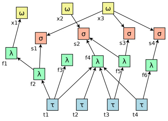
Figure 1.
A layered transport level view of the system showing, scheduled tasks (), stateless functions (), datasets (), and external applications ().
The intermediate layer is a backend infrastructure composed of stateless functions called by others or by edge devices. Unlike boxes, which are associated with real things, they are abstract and instantiated on demand. In Figure 1, such entities are represented as boxes. An arrow linking a box to a box represents the call of a function from an edge device. It is a static link, meaning that the sensor program contains a call to that function that it may or may not invoke during a specific run. Such layer is possibly thick, meaning that it may host chains of functions, as in the case of and in the example.
Anyway, a persistent state is needed to perform useful computation. In our model, it consists of shared persistent datasets, boxes in Figure 1. As a general rule, a dataset is not directly accessible by edge devices because of their constrained capabilities; an intermediate adapter function is therefore introduced. A dataset is a permanent entity, with a power consumption model which is similar to that of an edge unit: significant while processing a query, negligible during idle periods.
Interaction with external applications—the boxes in Figure 1—may happen in two directions. Internal s may obtain input from the outside of the system reaching external applications, or external applications can inspect the internal state of the system by querying the persistent records in boxes.
Figure 1 gives a static and application-level overview of the system. The lower network and link-level infrastructures are outside of the picture. The links are possibly built using constrained devices to minimize power consumption: for instance, with a combination of low-power and last-mile technologies.
In Figure 1, the arrows pointing to boxes represent the relationship that binds the caller to the calling function.
Arrows to and from external applications () are similar to those to/from s, with the difference that s are like black boxes outside of the system that may have an internal state.
To have a dynamic view of the system, we need to introduce a time coordinate, as shown in Figure 2. Each horizontal line represents the activity of a component: the color of the line is reminiscent of the color of the boxes in Figure 1, with the identifier on the left. The timing of the module is in the column on the right side. The figure represents the operation during one activity cycle of the edge unit . During the rest of the time—that may last minutes or hours—there is no operation related to .
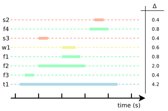
Figure 2.
An example of a time diagram of the activities triggered by . The color reminds the kind of activity: scheduled, function, dataset, or external. The right column indicates the activity duration in .
After a timed reboot, the operation of a sensor/actuator usually consists of
- downloading the last internal state,
- measuring environmental parameters,
- implementing an action, and
- uploading the new internal state.
The internal state retrieval and upload are carried out using s that help the to use datasets, possibly implementing complex functions like filtering the input with historical data. Likewise, when the action in step three depends on the system state, the returns to the calling a value, which determines its operation.
It emerges that, in the above model, the timing for the whole infrastructure is originated by edge devices. As a consequence, they cannot respond to network events without the latency determined by their activation period, which in our examples is in the order of minutes or hours. This constraint is consistent with communication patterns used in low-power WAN protocols: edge units radio is normally off, activated periodically for data delivery and command polling. For this reason, the power consumption of the overall infrastructure is tightly bound to the timing of devices. In the next section, we start from that timing to understand the energy footprint of the whole system.
3. Estimating Power Consumption
In our model, power consumption depends on time, with relatively short activity periods separated by long standby intervals.
A module follows the above pattern: while the module is active, its power consumption combines those of the processing unit and of the network interface (usually a radio), and drops of orders of magnitude in suspend mode. We indicate as the power consumption during the i-th activity period , respectively, when the module enters and leaves the suspend mode. Instead, the power consumption during standby periods is always the same, . The average power consumption during a time interval , i.e., the time between the two activity periods, is
To make the expression simpler, we introduce the duty cycle as the rate between the time interval during which the unit is active, and the period between two successive activities. The index k is that of the activity period:
Using the duty cycle, the expression for power consumption in a time interval between two activities is
Assuming all activity cycles are equal, i.e., same power consumption and duration (, we obtain an oversimplified but very intuitive expression:
Resuming the generic assumptions, the average power consumption of an activity triggered by the component is the sum of all those of the abstract functions and dataset queries that are in a causal relationship with the triggering event. We denote as the set of all modules that are instantiated as a consequence of the transition t. In the example in Figure 1:
To find the contribution of each function or query we evaluate its average power consumption during the edge unit activity interval . To simplify the notation, we assume that the lengths of activity intervals are constant for each given component x, and denoted with . For instance, in Figure 2, we have that and . Using this notation, the average power consumption of a generic dependent instance activity x during the activity of a component t is
And the overall power consumption of the activities triggered by the component is
with x ranging over all instances whose activation depends on the activity of the component.
The estimate of the overall power consumption is the sum of the above value with in expression (1):
Each activity cycle in the edge device requires at least one state retrieval from the dataset , so we need to take into account the energy footprint of this operation. When it is too frequent, the energy required by state retrieval may balance that saved thanks to the stateless approach. In that case, the designer should opt for a stateful solution.
The fine-grain comparison between stateful and stateless approaches is impossible as designs are quite different. A rule of thumb consists of comparing the average power consumption of networking operations for the serverless solution with that of the stateful one during standby. The rationale behind this is to compare the energy components that are present in only one approach: that spent for state retrieval, not needed in the stateful approach, and that spent when idling, which is null for the stateless approach.
To compute the first value, we associate each arrow in the dependency graph with the energy required by a data transfer. It is the product between the time to complete that operation, and the power consumption of the networking infrastructure serving the device. To compute the power consumption of a given , let be the time duration of the k-th arrow in its dependency graph, and be the power consumption of the gateway. The average power during an activation interval of the is
The other term of the comparison is the average power consumption during the idling time when the unit is not stateless. Indicating with the power consumption during a stateful wait we obtain
In conclusion, the stateful operation should be considered as more energy saving when the following condition holds,
As the duty cycle is necessarily smaller than one, we can simplify as
which is a threshold value for the time between two successive events on the unit. A stateful approach is preferable when the application exhibits an interval between events which is lower than the threshold.
Such a conclusion holds as long as the power consumption of the communication infrastructure is proportional to traffic. Otherwise, the above rule is not valid, and the stateful approach is less appealing since the traffic for state retrieval has no energy footprint.
3.1. Example
For instance, in Figure 1, assume that the edge device sets a one hour () timeout each time it enters the suspend mode. We assume that the edge device consumes when active [13], and when suspended, and that each module instance consumes during operation [14]. The for each module are given in Figure 2. Then we derive the following.
In the last line, we have the three components of the average power consumption: that of the component in sleep mode (1 mW) and during activity (0.45 mW), and the aggregate one for cloud resources (37.14 mW). We note that the cloud footprint dominates the total, which is welcome since cloud resources are not subject to tight power restrictions like edge units. However, this indicates that cloud resource management is a primary concern for the sustainability of an IoT application.
The example does not take into account the contribution of the networking infrastructure, but other models in the literature are very accurate in this respect, as explained in the next section. It is possible to extend our model by integrating such results.
We now apply the criteria in expression (4) to evaluate the suitability of a stateless approach for our example. For this, we assume that the roundtrip times of the seven requests are all ms, and that power consumption during communication is the same as that of a virtual host ( = 20 W). The power consumption of an edge unit in stateful suspend mode is mW. It is significantly lower than as the radio and other power-consuming components are switched off. Under such assumptions, the criterion does not hold by two orders of magnitude, and then the stateless approach is more convenient.
Finally, we observe that a stateful approach becomes convenient when the interval between successive events is less than one minute.
4. Discussion
This section addresses three aspects of the proposed model. In the first place, we explain why a FaaS provision suits an IoT application and the relationship with the stateless computational model. Next, we consider the practical availability of the parameters used for model configuration and, finally, we analyze its security aspects.
We introduce a computational model that precisely targets IoT designs. Given concise and practically available attributes of system components, the model wants to predict the energy footprint of the system.
To target IoT systems, we consider that edge devices are constrained devices spending most of the time in a deep-sleep mode to save energy. The model defines them as components, associated with a schedule and variable energy consumption. The units are stateless as they lose their internal state when switching to deep-sleep. The backend of the system is composed of short-lived virtual resources that perform a simple task and are immediately de-allocated. The model defines them as components, associated with a causal relationship with units and energy consumption. Also components are stateless, since they are de-allocated after execution, and their resources used otherwise. Serverless cloud provisions fit the definition of components. Finally, units are stateful components that represent the state of the system: only defined components hold the credentials needed to request them a transaction, which has an energy footprint similar to that of a .
The model limits its scope to the application layer: the entities that populate it are processes that exchange data among each other. Although the networking infrastructure (the transport layer and below) is outside the scope of that view, the model does not overlook its energy consumption. That of units originates from the communication equipment (usually a radio) and contributes to . The energy footprint of networking devices serving edge units is associated with the relationships (the arrows) between and components, and it depends on the sharing policy of such devices. The energy consumption of communication between and units depends on the cloud infrastructure, and is also associated with the dependencies among such components.
An issue that our model shares with any other quantitative one is the practical availability of the parameters that define the model.
It is a minor concern for the parameters related to the components since they are available by measurement (as in the case of the ) or examining log records. To this end, the service provider supplies the designer with data that are useful to estimate the energy footprint of components. For instance, the MongoDB Stitch service provides a log of execution times of all function calls (which inspires the values in Figure 2).
Parameter availability for the backend network is a concern when it involves a cloud infrastructure. In that case, a link-layer model of the system may help.
In 2017, Ahvar et al. published a detailed model for the energy consumption of Infrastructure as a Service (IaaS) cloud computing infrastructures [15]. They focus on the link-layer view of the system, categorizing the topology depending on the amount of computation on end-user premises, and compare the energy footprint of different design approaches.
They define a very detailed model for energy consumption, including, the contribution of computing resources, but also that of the networking devices that route data from the edge to the core and vice versa. The model splits energy consumption into a static and a dynamic part. The former relates to idling units, i.e., running with no load or in standby, while the latter refers to busy ones. The dynamic load model of the networking infrastructure is packet-wise and reflects its effective utilization.
The authors warn that the precision of the model degrades since resource sizing considers peak conditions, and then the allocated computing power is frequently in excess. As a consequence, power consumption estimates become difficult, and the allocation model incurs a substantial waste of computing power.
Simulating a generic scenario, the authors conclude that networking devices are responsible for static power consumption (circa 90%). In contrast, the power consumption of physical servers dominates the dynamic power consumption.
This result nicely fits into our model: if the overall energy consumption is approximately static, then the share of energy required by a message exchange is more available. Regarding the computing activity, the serverless paradigm assigns the task of optimizing the allocation of the function to the provider. The transient nature of s excludes their migration and facilitates task management. In conclusion, the two models exhibit complementary features, so we consider their integration as viable.
As a closing remark, there is a growing interest [15,16] for pricing models based on energy consumption. We may expect that, in the future, such figures will be even more available to the end-user.
Another reason for an association between IoT and serverless computing is related to security issues: let us explore how the proposed model deals with them, even without an explicit mention.
Security is a known issue in IoT systems [17]. Many factors contribute to their fragility on this respect, including the constraints on edge devices and protocols, and the presence of shared data.
Regarding attacks directed to edge devices, a fundamental principle of the model is that they operate intermittently. This option drastically reduces the time window for attacks; for instance, those that exploit Over The Air (OTA) capabilities [18].
Concerning the security issues related to shared data, the use of serverless functions avoids the exploits that target the internal state of cloud instances. On this subject, Alpernas et al. [19] discuss the application of serverless computing resources observing that “each invocation starts from a clean state and does not get contaminated with sensitive data from previous invocations”. In essence, a certified user invokes the function which makes controlled access to confidential data, and finally returns a result to the same user.
The model is agnostic about the communication protocol serving edge devices: therefore, it is the responsibility of the designer to address a stack that guarantees a suitable level of security. In 2016, Dan Dragomir et al. [20] listed fifteen of them, each with specific security issues and solutions. It is an extremely active research front with new results continuously appearing. In the concluding use-case, we adopt a stack WiFi + SSL + HTML, which exhibits a security/versatility tradeoff.
5. Use Case and Prototype Solution
We discuss a use case to give an insight into stateless design principles. We also aim at demonstrating two features of the model:
- the ability to represent a simple use case: this indicates that the model is expressive enough to be used in practice, and
- the availability of the parameters: as discussed above, this is a challenging aspect, because not all of them are directly observable.
To make the use case realistic, we introduce a problem and a complete solution. We do not discuss design alternatives: the solution we propose is just valid for the purpose, without claims of optimality. We use the model to discuss a weaker property that we call sustainability, which means that the control system consumes less than the controlled device. It gives us a way to exercise the model towards a concrete result. We proceed in two steps: first, we describe the solution using our notation; next, we compute and discuss its energy footprint.
As the operational parameters are similar to those used in the example in Section 3.1, there is no point in re-calculating the threshold value to find that a stateless approach is suitable. Instead, we use the model to compare the power consumption of the controlled device—a water pump—and that of the controller. We try to define the limits of the proposed solution and to find alternatives.
5.1. Use Case Description
The use case is similar to that described in AWS documentation [21], and deals with a typical plant watering system:
The system is composed of several independent plants. Each of them uses an electrical pump that takes the water from distinct tanks. Each plant operates at a predetermined hour to avoid stress to the crops and overloads to the power distribution. The duration of watering is computed depending on weather conditions. The weekly history of the watering system is available in a dashboard, which also warns the user when a tank is empty. The configuration of each plant is under the control of authenticated users.
5.2. Materials
The functional device is a 12 V, 10 W pump connected to an actuator that we implemented starting from a WEMOS D1 mote. The project is available on line with the details of the software [22].
The WEMOS device operates at 3.3 V and embeds an MCU with a WiFi transceiver. On the same board, see Figure 3, a relais controlled by the MCU operates the pump. A step-down converter transforms the 12 V power to 3.3 V to feed the controller. To monitor the water level the device measures the current in the motor, which is significantly lower when the tank is empty.
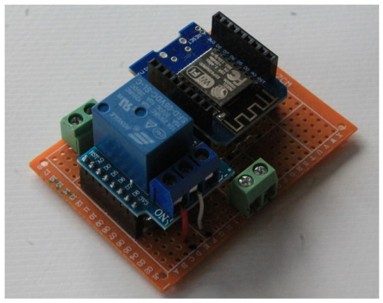
Figure 3.
The prototype board, with the WeMos and the relay.
The WEMOS has various suspend modes; the most effective one is called “deep sleep” and shuts down the entire device except a timer that reboots it after a given timeout. The timer has a limited capacity and accuracy, and therefore the suspend time cannot exceed one hour with 10% precision.
The network infrastructure serving edge devices consists of a WiFi LAN connected to the Internet by a commercial AP.
The Functions and the Datasets are implemented using MongoDB services.
5.3. Mapping the Model on MongoDB
Figure 4 shows the functional modules that implement our solution for the use case. The MongoDB Stitch service hosts the boxes, which are JavaScript functions invoked through HTTPS API. The modules, the MCU of which is powerful enough to implement the HTTPS protocol, interact with modules using such an interface. As the Stitch interface uses standard RESTful HTTP requests, there is no need to import a specific MongoDB library in the WEMOS sketch.
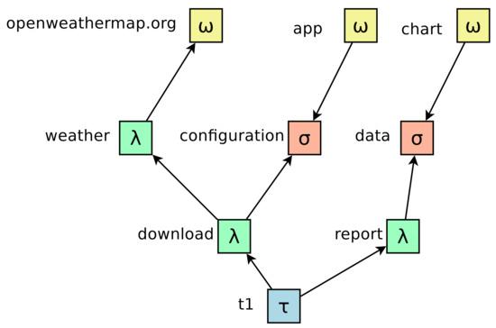
Figure 4.
The functional modules that implement the prototype solution for the use case.
Besides receiving requests from modules, Stich Functions (“functions” in the rest of this article) are callable by other functions, which allows building a thick function layer. Functions can also call external services, thus implementing outbound arrows like .
The datasets that store the system state—the boxes in our model—are MongoDB collections: each box is a different collection. MongoDB is a NoSQL database, expressly designed for scalability and flexibility. Functions make access to the database using a specialized library.
External services have access to the datasets of the application by accessing the MongoDB collections where they are stored; user credentials enforce an appropriate security level.
5.4. Use Case Implementation Details
To enforce low-power operation in the edge unit, we use the “deep sleep” suspend mode. We cannot set a day-long sleep interval since the hardware limits the length of a deep-sleep period to little more than one hour. Therefore, every time the mote wakes up from deep sleep, it calls the download function (detailed below), which returns the time left before next watering; depending on such value the device either suspends for another hour or for the remaining time if it is less than one hour.
The download function issues a query to the configuration dataset to obtain the attributes of the plant, including the watering hour. Note that each edge unit has its identifier hardwired in the code to find the document in the dataset. The download function also calls an external weather function, which queries an external weather service and computes the duration of the watering. Finally, the download function returns the edge unit a JSON structure containing the time left to wait, and the duration of the watering.
At the end of the watering activity, the edge unit uploads a report with the measurement of the motor current for monitoring the tank level and the effective duration of the watering. Such information is encoded in a URL calling the report function (see Figure 5), which formats the data in a JSON object together with the identifier of the edge unit and uploads it in the data collection.
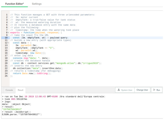
Figure 5.
The JavaScript source of the report Stitch Function as displayed in the IDE provided by the Atlas web interface.
All function calls are protected using a secret code—a symmetric key—in the header of the request. Security can be further increased using a content signature to ensure the validity of the data, and HTTPS to ensure the identity of the server. MongoDB Stitch supports all such mechanisms.
In analogy, Reichherzer et al., addressing IoT systems for home automation, introduce four categories for system security and scalability [23]:
- minimal security/no scalability,
- basic security/no scalability,
- basic security/scalable authentication, and
- scalable web service/scalable authentication.
The design of our demo falls in the fourth category, which is the one the authors indicate as the best for system security and scalability. For their testbed, they use the serverless provision and authentication mechanisms of AWS instead of Atlas MongoDB ones.
A Web application uses the MongoDB Chart service to obtain a graphical representation of the report collection for a given plant. MongoDB Atlas allows identified users to modify the configuration collection. For instance, modifying the watering time, or the hour, or the parameters that regulate its duration.
5.5. Energy Consumption Analysis
The energy consumption of the whole system is the aggregate of the contributions of all plants; in this section, we analyze the apport of a single plant. From that analysis, we aim at understanding how the power consumption of the control system (including the control board and the cloud resources) compares with that of the controlled device, the water pump: we would like to ensure that the controller consumes less than the worker.
We proceed in three steps. First, we consider the power consumption of the edge layer, evaluating the share of power consumed by control electronics compared with that of the functional device, the watering pump. Next, we analyze the power consumption of the networking devices serving the edge layer, and, finally, that of cloud instances.
We measured the current drawn by the board from the 12 V power input during deep sleep, and during activity. In the first case it is stable at 300 A, while during activity it is 25 mA, with a power consumption of 3.6 mW and 300 mW, respectively.
The timing of the system is such that a one day cycle consists of twenty-three one hour periods followed by a shorter one; each of them terminates with a call to the download function. At the end of the last one, the MCU powers the pump for the required time and finally invokes the report function.
The duration of the hourly activity has been measured and is generally less than 30 s long: it embeds the AP join, and the HTTP session that invokes the download function.
The daily operation has a variable duration since the watering pump lapse varies depending on weather conditions and other details: a watering of minutes is sufficient in a residential house, not in an open field [24]. We indicate with the duty cycle of the pump, which corresponds to the rate between the activation lapse and the period, which is of one day.
The aggregate duration of the hourly cycles and the final activation cycle determines the duty cycle d of the controller, and so we leave such a parameter variable in our study. Using Equation (3), we obtain an average power consumption estimate that depends on the duty cycle:
whereas the average power consumption of the 10 W watering pump depends on the watering pump duty cycle :
When their rate is lower than one, we are in a situation where the pump consumption dominates the total, that we consider as sustainable. In our case:
The controller is active when it controls the pump, and during the time spent in communicatio before and after watering. Therefore we decompose the d in a component and in the sum of twenty-four periods 30 s long, so that
and we obtain a threshold value for the duty cycle of the pump:
As the cycle is one day (i.e., 86,400 s) long, the threshold value for the watering duration is of 57 s every day. If the watering duration is above that threshold, thus excluding very small scale plants, the design meets our sustainability principle (as defined in Section 5) since the power consumption of the appliance dominates that of the control system.
To refine the evaluation of the stateful operation, we observe that, using a standby mode that preserves the state of the MCU (called “modem sleep”), the power consumption of the board is 120 mW. With the same computations seen above, we obtain a threshold value for sustainability which is greater than 17 m.
The energy consumption of the Access Point (AP) plays a different role: assuming that the device serves only the watering system, all connected edge units share its power consumption.
Let an AP with a power consumption of 5 W serve an area covered by ten plants: then each plant participates with an average of 0.5 W. In that scenario, the duty cycle to balance the power consumption of the pump is approximately one hour per day: it is one order of magnitude higher than that obtained considering only the power consumption of edge units. Let us find a way to reduce such value.
One is to increment the number of plants per AP, but this is not viable due to its limited coverage, which cannot be filled up with much more than ten plants. As an alternative, consider that the AP participates in other services: for instance, a public WiFi service in a residential area. In that scenario, the energy footprint of a single plant, corresponding to twenty-four HTTP sessions per day, is negligible.
The evaluation of the energy consumption of the system in the MongoDB cloud is even fuzzier. We extract from the log the CPU-time for each transaction (see Figure 6). It is the same value for a download and a report, approximately 400 ms. Given that the download function is called once per hour, and the report and weather once a day, we obtain a CPU-time of 30 s per day per plant, corresponding to a cloud duty cycle of . Now, we need to estimate the power consumption of the container for the function. We assume that, when scheduled, it is the only process running on the server: typical power consumption for such a device is of 20 W. From the duty-cycle, we infer an average power consumption of 7 mW. We are now able to compute the threshold value for sustainability, which corresponds to a duty cycle of , near to that we found for edge units.
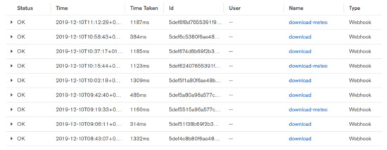
Figure 6.
An example of the log file available on the Atlas Web interface. The third column shows the execution time of the function indicated in column six.
In conclusion, edge devices and cloud FaaS resources have similar energy footprints. To exhibit a comparable one, the water pump needs to operate at least a minute per day. The network infrastructure serving the edge devices is critical: if it is used by the watering plant only, its footprint dominates that of the others by one order of magnitude.
6. Conclusions
We introduce the tools to design and analyze systems that use stateless components. Their use may bring to a significant energy saving, especially in the design of IoT systems, and improves system security. Our approach includes, besides stateless edge devices, also stateless distributed software components implemented using serverless cloud applications. This feature contributes to the originality of our approach because their availability as cloud resources is recent, and their inclusion in an abstract model is new.
We introduce two graphical tools: one to represent the dependencies among system components, another for the timing of the asynchronous operation of the system. Stateless edge devices trigger events controlling other units. The state of the system is secured in dedicated storage.
As we are mostly interested in energy-related issues, which are of paramount importance for IoT systems, we introduce a simple model to compute the energy footprint of the system. We use that model to find the limits of the stateless approach; when certain conditions hold, a stateful one is preferable. We discover that such limits depend on the efficient use of the link-layer infrastructure that serves edge devices. When the link layer is dedicated, the stateless approach improves its utilization, which remains sub-optimal. The most suitable option consists of sharing the infrastructure.
We study a simple use case to prove the applicability of our framework. The use case consists of a system that controls the watering of an farming plant. The implementation of the whole system uses stateless components for the hardware edge devices and the cloud components. Using the energy footprint model, we evaluate the suitability of a stateless approach, and we compare the energy footprint of the controlled devices—the watering pumps—with that of the control system. Again, we discover the weight of the link-layer infrastructure.
As the tools for the implementation of stateless, asynchronous system components are quite young, we expect rapid growth of the commercial offer regarding this approach. The presence of a simple model for the description of such architectures may foster interoperability and simplify their design. The present work goes in that direction. Further steps are the building of an integrated development environment that facilitates the management of the design lifecycle, including its deployment. As the link-layer infrastructure plays an essential role in defining the energy footprint, the model should be extended in that sense, taking into account technologies that allow an asynchronous, on-demand operation.
Funding
This research received no external funding.
Conflicts of Interest
The author declares no conflict of interest.
References
- Sittón-Candanedo, I.; Alonso, R.S.; García, O.; Muñoz, L.; Rodríguez-González, S. Edge Computing, IoT and Social Computing in Smart Energy Scenarios. Sensors 2019, 19, 3353. [Google Scholar] [CrossRef] [PubMed]
- Celesti, A.; Mulfari, D.; Fazio, M.; Villari, M.; Puliafito, A. Exploring Container Virtualization in IoT Clouds. In Proceedings of the 2016 IEEE International Conference on Smart Computing (SMARTCOMP), St. Louis, MO, USA, 18–20 May 2016; pp. 1–6. [Google Scholar] [CrossRef]
- Pahl, C.; Helmer, S.; Miori, L.; Sanin, J.; Lee, B. A Container-Based Edge Cloud PaaS Architecture Based on Raspberry Pi Clusters. In Proceedings of the 2016 IEEE 4th International Conference on Future Internet of Things and Cloud Workshops (FiCloudW), Vienna, Austria, 22–24 August 2016; pp. 117–124. [Google Scholar] [CrossRef]
- Jock, R. Serverless at the Edge: Up and Running w/OpenFaaS & Docker on a Raspberry Pi Multi-Node Cluster with PiBakery. Available online: https://medium.com/@JockDaRock/serverless-at-the-edge-up-and-running-w-openfaas-docker-on-a-raspberry-pi-multi-node-cluster-e0957f4d8a49 (accessed on 26 July 2019).
- Mohanty, S.K.; Premsankar, G.; di Francesco, M. An Evaluation of Open Source Serverless Computing Frameworks. In Proceedings of the 2018 IEEE International Conference on Cloud Computing Technology and Science (CloudCom), Nicosia, Cyprus, 10–13 December 2018; pp. 115–120. [Google Scholar] [CrossRef]
- Lee, K.; Kim, Y.; Yoo, C. The Impact of Container Virtualization on Network Performance of IoT Devices. Mob. Inf. Syst. 2018, 2018, 9570506. [Google Scholar] [CrossRef]
- Ciuffoletti, A. OCCI-IoT: An API to Deploy and Operate an IoT Infrastructure. IEEE Internet Things J. 2017, 4, 1341–1348. [Google Scholar] [CrossRef]
- Persson, P.; Angelsmark, O. Kappa: Serverless IoT Deployment. In Proceedings of the 2nd International Workshop on Serverless Computing, Las Vegas, NV, USA, 11–12 December 2017; ACM: New York, NY, USA, 2017; pp. 16–21. [Google Scholar] [CrossRef]
- AWS Serverless Application Model. Available online: https://aws.amazon.com/it/serverless/sam/ (accessed on 26 July 2019).
- Open Source Serverless Cloud Platform. Available online: http://openwhisk.apache.org/ (accessed on 26 July 2019).
- Boyd, M. Managing State in Serverless. Available online: https://thenewstack.io/managing-state-in-serverless/ (accessed on 26 July 2019).
- Ahvar, E.; Orgerie, A.; Lébre, A. Estimating Energy Consumption of Cloud, Fog and Edge Computing Infrastructures. IEEE Trans. Sustain. Comput. 2019, 1–12. [Google Scholar] [CrossRef]
- ESP8266EX Datasheet. Available online: https://www.espressif.com/sites/default/files/documentation/0aesp8266ex_datasheet_en.pdf (accessed on 2 January 2020).
- Callau-Zori, M.; Samoila, L.; Orgerie, A.C.; Pierre, G. An experiment-driven energy consumption model for virtual machine management systems. Sustain. Comput. Inform. Syst. 2018, 18, 163–174. [Google Scholar] [CrossRef]
- Narayan, A.; Rao, S. Power-Aware Cloud Metering. IEEE Trans. Serv. Comput. 2014, 7, 440–451. [Google Scholar] [CrossRef]
- Aldossary, M.; Djemame, K. Energy Consumption-based Pricing Model for Cloud Computing. In Proceedings of the 32nd UK Performance Engineering Workshop, Bradford, UK, 8–9 September 2016; pp. 16–27. [Google Scholar]
- Alaba, F.A.; Othman, M.; Hashem, I.A.T.; Alotaibi, F. Internet of Things security: A survey. J. Netw. Comput. Appl. 2017, 88, 10–28. [Google Scholar] [CrossRef]
- Zandberg, K.; Schleiser, K.; Acosta, F.; Tschofenig, H.; Baccelli, E. Secure Firmware Updates for Constrained IoT Devices Using Open Standards: A Reality Check. IEEE Access 2019, 7, 71907–71920. [Google Scholar] [CrossRef]
- Alpernas, K.; Flanagan, C.; Fouladi, S.; Ryzhyk, L.; Sagiv, M.; Schmitz, T.; Winstein, K. Secure serverless computing using dynamic information flow control. Proc. ACM Program. Lang. 2018, 2, 1–26. [Google Scholar] [CrossRef]
- Dragomir, D.; Gheorghe, L.; Costea, S.; Radovici, A. A Survey on Secure Communication Protocols for IoT Systems. In Proceedings of the 2016 International Workshop on Secure Internet of Things (SIoT), Heraklion, Greece, 26–30 September 2016; pp. 47–62. [Google Scholar] [CrossRef]
- AWS IoT Plant Watering Sample. Available online: https://docs.aws.amazon.com/en_us/iot/latest/developerguide/iot-plant-watering.html (accessed on 26 July 2019).
- Ciuffoletti, A. Low-Power Watering with a WEMOS. 2019. Available online: https://hackaday.io/project/166819-low-power-watering-with-a-wemos (accessed on 3 February 2020).
- Reichherzer, T.; Mishra, A.; Kalaimannan, E.; Wilde, N. A Case Study on the Trade-Offs between Security, Scalability, and Efficiency in Smart Home Sensor Networks. In Proceedings of the 2016 International Conference on Computational Science and Computational Intelligence (CSCI), Las Vegas, NV, USA, 15–17 December 2016; pp. 222–225. [Google Scholar] [CrossRef]
- Kustas, W.; Agam, N. Soil evaporation. In Encyclopedia of Natural Resources; Chapter Soil Evaporation; Wang, Y., Ed.; Taylor & Francis: Boca Raton, FL, USA, 2014; p. 10. [Google Scholar] [CrossRef]


© 2020 by the author. Licensee MDPI, Basel, Switzerland. This article is an open access article distributed under the terms and conditions of the Creative Commons Attribution (CC BY) license (http://creativecommons.org/licenses/by/4.0/).