Article

Penalty-Enhanced Utility-Based Multi-Criteria Recommendations

Department of Information Technology and Management, College of Computing Illinois Institute of Technology, Chicago, IL 60616, USA
Information 2020, 11(12), 551; https://doi.org/10.3390/info11120551
Submission received: 18 October 2020 / Revised: 15 November 2020 / Accepted: 20 November 2020 / Published: 26 November 2020
(This article belongs to the Special Issue Information Retrieval and Social Media Mining)

Abstract

:
Recommender systems have been successfully applied to assist decision making in multiple domains and applications. Multi-criteria recommender systems try to take the user preferences on multiple criteria into consideration, in order to further improve the quality of the recommendations. Most recently, the utility-based multi-criteria recommendation approach has been proposed as an effective and promising solution. However, the issue of over-/under-expectations was ignored in the approach, which may bring risks to the recommendation model. In this paper, we propose a penalty-enhanced model to alleviate this issue. Our experimental results based on multiple real-world data sets can demonstrate the effectiveness of the proposed solutions. In addition, the outcomes of the proposed solution can also help explain the characteristics of the applications by observing the treatment on the issue of over-/under-expectations.

1. Introduction

Information retrieval and recommender systems are two solutions to alleviate the problem of information overload [1], while recommender systems can deliver personalized recommendations to the end users without users’ explicit queries. Recommender systems are usually built by learning from different types of the user preferences, such as explicit ratings or implicit feedbacks [2,3]. In the past decades, different types of the recommender systems have been proposed and developed. Multi-criteria recommender systems (MCRSs) [4] is one of these recommender systems which take the user preferences on different aspects of the items into account to improve the quality of the recommendations.
MCRSs have been implemented and served in real-world applications, such as hotel bookings at TripAdvisor.com, movie reviews at Yahoo!Movie, restaurant feedbacks at OpenTable.com. An example of the OpenTable.com can be shown by Figure 1. The system allows users to reserve tables at a restaurant and leave ratings on their dinning experiences. To review user experiences on a restaurant, we are able to observe the overall rating and multiple ratings on different aspects of the restaurant in Figure 1b, such as food, service, ambiance and noise level. It is because the system collects each user’s overall rating and multi-criteria ratings as shown by Figure 1a. Afterwards, MCRSs can be built by taking advantage of these multi-criteria ratings in order to deliver more effective restaurant recommendations.
An example of data in MCRSs can be shown by Table 1. The rating refers to the users’ overall rating on the items. We also have users’ ratings on multiple criteria, such as food, service and value.
The research problem in MCRS is straightforward. Take the task of rating predictions for example; MCRSs predict an overall rating for a user and an item by taking advantage of the user’s multi-criteria ratings on the item. In Table 1, MCRSs try to predict U 3 ’s overall rating on T 1 as shown in the table above, while we do not know U 3 ’s multi-criteria ratings on T 1 . Usually, we need to estimate a user’s multi-criteria ratings on an item, and then aggregate these ratings to finally predict the overall rating. The predicted overall rating can be used as a ranking score to sort and produce the list of recommendations delivered to the user.
Most recently, a utility-based multi-criteria recommendation approach [5] was proposed and it was demonstrated as one of the most effective methods. In this approach, we assume that there are user expectations on the items which can be represented by a list of ratings in multiple criteria. Given an item, we can also estimate a user’s ratings on the different aspects of the items. In this case, the similarity between the user expectations and the multi-criteria ratings on the items can be considered as the utility of the item from the perspective of the user. A user may like the items more, if the similarity between user expectation and the user’s multi-criteria ratings on these items is higher. The similarity score therefore can be used to rank the items to produce the top-N recommendations. We proposed to learn these user expectations by a learning-to-rank [6,7] method, and the experimental results were effective and promising.
However, there is a drawback in this approach. Namely, there is an issue of over-/under-expectations, while the current utility or similar function is not able to capture it. The issue refers to the situation that a user’s rating on an item may lead to over-/under-expectations in comparison with the user’s expectations on the items. Finally, It could result in false positives in the recommendation list and false negatives in the recommendation candidates. Take Table 2 for example, the first three rows refer to user u’s rating vectors on three items, while the last row refers to u’s expectations to select a restaurant to dine in. It is clear that u’s ratings on T 1 are under-expectations, while his or her ratings on T 2 are over-expectations. However, some of u’s ratings on T 3 are under-expectations, while others are over-expectations. It results in the difficulty of deciding whether the user will like T 3 . It could be more complicated when it comes to the recommendation methods in the proposed utility-based multi-criteria recommendation models. A filtering strategy [8] may be helpful to alleviate the issue, but we need to pre-define the filtering rules by using domain knowledge. The challenge, therefore, becomes how to figure out a general solution for the utility-based multi-criteria recommendation model without domain knowledge.
In this paper, we propose to learn and apply penalties for the situation of over-/under-expectations. The proposed solution is generally enough to be applied in any applications, and we do not need any domain knowledge to define the filtering rules. The experimental results based on multiple data sets can demonstrate the effectiveness of our proposed solutions.
The remainder of this paper is organized as follows. Section 2 positions the related work. Section 3 presents the utility-based multi-criteria recommendation model. Section 4 discusses our proposed solution to alleviate the issue of over-/under-expectations. Section 5 presents the experimental results, followed by the conclusions and future work in Section 6.

2. Related Work

In this section, we discuss the related work in multi-criteria recommender systems, as well as the utility-based recommendation models.

2.1. Multi-Criteria Recommendations

As mentioned before, we have both overall rating and multi-criteria ratings in the rating data. The task in MCRS is predicting the overall rating for a user on an item by taking advantage of the multi-criteria ratings. Usually, we need to estimate a user’s multi-criteria ratings on an item, and then aggregate these ratings to finally predict the overall rating, as shown in Equation (1). We use R 0 to represent the overall rating, and R 1 , 2 , , k as the multi-criteria ratings, while the function f is denoted as the aggregation function.
R 0 = f ( R 1 , R 2 , , R k )
Several multi-criteria recommendation algorithms have been developed to take advantage of these multi-criteria ratings. One of these methods is the heuristic approach [4,9] which utilizes the multi-criteria ratings to better calculate user-user or item-item similarities in the collaborative filtering algorithms. Another one is the model-based approach [4,10,11] which constructs a predictive model to estimate a user’s overall rating on one item from the observed multi-criteria ratings. The model-based methods are usually more effective than the heuristic approach, since they are machine learning based algorithms which can even alleviate sparsity issues in the rating data.
Adomavicius, et al.’s [4] linear aggregation is one of the most basic and popular model which is usually utilized as a baseline for the purpose of benchmark. In this approach, we need to predict a user’s rating on each criterion independently by using any rating function in the traditional recommender systems. Afterwards, we can use a linear regression as the aggregation function to finally estimate the overall rating by taking advantage of these predicted multi-criteria ratings.
One drawback in the approach above is that it ignores the correlation among the different criteria. Take the restaurant recommendation in the OpenTable for example, a user may not give a high rating on the criterion “value”, if the user does not like the “food” in this restaurant. Researchers try to build more effective models by taking the correlation of the criteria into considerations. The flexible mixture model [10] is one of these attempts. It is a mixture model-based collaborative filtering algorithm incorporating the discovered dependency structure, while multiple criteria can be put on the structure connected with a user and an item by using two latent variables. We made another attempt and proposed the approach of criteria chains [11], in which we predicted the multi-criteria ratings in a sequence. The predicted preference in one criterion could be considered as contexts to be used to predict the preference in the next criterion. In this way, we were able to consider the correlation among criteria in the chain.

2.2. Utility-Based Recommendation Models

According to the classification of recommender systems by Burke [12], there are five categories—collaborative models [13,14], content-based recommenders [15,16], methods which utilize demographic information [17], knowledge-based algorithms [18,19], and utility-based models [5,20,21]. The utility-based recommenders make suggestions based on a computation of the utility of each item for the user. Utility can be used to indicate how valuable an item is from the perspective of a user. The utility function may vary from data to data, and there are no unified function to be generalized to different domains or applications. Guttman used different transformation functions (e.g., linear, square or universal functions) for different types of the attributes (e.g., continuous or discrete) in the context of online shopping [20]. Li et al. [22] defined the utility of recommending a potential link in the social networks by a linear aggregation of its value, cost, and the linkage likelihood. Moreover, Zihayat et al. proposed to use the aggregation of article-driven (e.g., popularity, topic distributions) and user-driven measures (e.g., clickstream, dwell time) as the utility function for news recommendations [21]. The utility-based multi-criteria recommendation model [5] discussed in the next section is an example which designs the utility function to serve multi-criteria recommendations. Different optimization methods can be applied to find the optimal solution in the utility-based recommendation model. A multi-objective optimizer [23,24] could be useful, if there are multiple objectives involved in the recommendation model.
Our previous work [5] proposed and developed the utility-based multi-criteria recommendation models. However, we ignored the over-/under-expectation issue. In this paper, we propose the improved solutions which are built upon the previous model but they further alleviate the issue of the over-/under-expectations.

3. Preliminary: Utility-Based Multi-Criteria Recommendations

In this section, we introduce the existing utility-based multi-criteria recommendation model [5].

3.1. Utility-Based Model (UBM)

The major contribution of our previous work [5] is the design of the utility function for the multi-criteria recommender systems. More specifically, the utility of an item from the perspective of the user refers to how valuable the item is in view of a user. It was defined as the similarity between the vector of user expectations and the vector of user ratings in the multiple criteria (i.e., different aspects of the items).
Assume there are N criteria, we use c u to represent the vector of user expectations for a user u, and r u , i denotes the u’s rating vector (i.e., multi-criteria ratings) on the item i, as shown in Equations (2) and (3). Note that the expectation vector tells a user’s expectations on the favorite items aligned to the same criteria used in the vector r u , i . More specifically, r u , i t (t = 1, 2, ⋯, N) refers to user u’s rating on the item i in the t th criterion. Accordingly, c u t can tell user u’s expectation on the items in terms of the t th criterion. They must be in the same rating scale for each criterion.
c u = < c u 1 , c u 2 , , c u N >
r u , i = < r u , i 1 , r u , i 2 , , r u , i N >
The value of the utility can be obtained by the similarity or distance measures between two vectors, as shown in Equation (4). The larger the utility is, the more the user may like this item. Note that distance measure will represent dissimilarities, since the similarity will be higher if the distance is smaller.
U t i l i t y ( u , i ) = s i m i l a r i t y ( c u , r u , i )
Theoretically, any similarity measures can be applied in Equation (4), such as Pearson correlation, cosine similarity, or distance measures (e.g., Manhattan distance, Euclidean distance, etc.) as dissimilarity measures. Our research deliver more insights about these similarity measures. First of all, Pearson correlation may not be a good choice since the values may not be reliable if the number of dimensions in the vectors is limited. In the area of MCRS, we usually have three or four multiple criteria, which raises the concerns in Pearson correlation. In addition, the angle-based measures, such as the cosine similarity, are not appropriate, since it may produce 100% similarity if two vectors are parallel but with different values. As a result, the distance measures can be utilized to represent the dissimilarity. Any distance measures can be applied. We tried both Manhattan distance and the Euclidean distance, and found that we could get better results by using Euclidean distance. Therefore, we only present the results based on the Euclidean distance in this paper. The distance values should be normalized to the unit scale, and then we use 1 minus the normalized distance value to represent the similarity between the two vectors.
Therefore, the workflow in the utility-based recommendation model can be summarized as follows. We use the data in Table 1 for example, and our task is to produce the top-N recommendations to user U 3 .
First of all, we need to make predictions on the multi-criteria ratings in order to obtain the vector of user ratings on the items, i.e., r u , i . In other words, we need to predict how U 3 will rate all candidate items on the three criteria, {food, service, value} in Table 1. In our work, we apply a process of independent predictions. More specifically, to predict how how U 3 will rate an item on the criterion “service”, we will apply a traditional recommendation algorithm on the rating matrix <user, item, service>. Accordingly, we apply the same algorithm on other rating matrix associated with the ratings on each criterion. We use biased matrix factorization (BiasedMF) [25] as the recommendation algorithm in this step, since it is usually considered as a standard baseline and effective algorithm in the traditional recommender systems.
The rating prediction function by BiasedMF [25] can be shown in Equation (5).
r ^ u i = μ + b u + b i + p u T q i
μ refers to the global average rating, while b u and b i are the user bias and item bias respectively. p u and q i are the latent-factor vector which can represent u and i respectively. The MF will learn these parameters by minimizing sum of squared errors by using stochastic gradient descent as the optimizer. The L 2 norms are usually added into the loss function as the regularization terms in order to alleviate overfitting. The loss function is described in Equation (6), where λ is the regularization rate. r u i and r ^ u i are the real rating and predicted rating for the entry u , i . The model will learn from each entry u , i in the training set T. We use p * , q * , b * to represent the user latent-factor vectors, item latent-factor vectors and biases respectively which are the parameters to be learned in the process of optimizations.
M i n i m i z e p * , q * , b * ( u , i ) T ( r u i r ^ u i ) 2 + λ ( | | p u | | 2 + | | q i | | 2 + b u 2 + b i 2 )
Once we obtain the users’ predicted multi-criteria ratings on the items, we randomly initialize the expectation vector for each user, and learn these vectors by using the optimization below.

3.2. Optimization

We can initialize user expectations for each user at the beginning. In this case, we are able to use Equation (4) to calculate the utility score which will be used to rank the items to produce the top-N recommendations. Our previous work [5] learns these user expectations by maximizing the normalized discounted cumulative gain (NDCG) [26] which is a metric used for listwise ranking in the well-known learning-to-rank methods. Assuming each user u has a “gain” g u i from being recommended an item i, the average discounted cumulative gain (DCG) for a list of J items is defined in Equation (7).
D C G = 1 N u = 1 N j = 1 J g u i j m a x ( 1 , l o g b j ) )
where the logarithm base is a free parameter, typically between 2 and 10. A logarithm with base 2 is commonly used to ensure all positions are discounted. NDCG is the normalized version of DCG given by Equation (8), where D C G * is the ideal DCG, i.e., the maximum possible DCG.
N D C G = D C G D C G *
In terms of the listwise ranking, LambdaRank [27] can be applied to optimize NDCG directly. In addition, genetic and evolution algorithms have also been demonstrated as effective solutions in the listwise ranking optimization [28]. They have been utilized as the optimizer in the area of recommender systems before [29,30]. Our previous work found particle swarm optimization (PSO) [31] to be an effective optimizer, and it is easy to be implemented.
The basic workflow in the PSO can be described by Algorithm 1. In PSO, we need to initialize multiple particles to search for the optimal solution, while we use the NDCG shown in Equation (8) as the fitness function. The position of each particle is the parameters we need to learn. In our case, the position here refers to the all of the user expectation vectors. At the initialize stage, we need to define the number of particles, the initial positions and velocity. The velocity can define how much each particle can move (i.e., change the positions at the beginning).
Algorithm 1: Workflow in PSO.
Information 11 00551 i001
Each particle will run the algorithms with the initialized positions (i.e., user expectations) and velocity. The velocity is a vector with the same size of the position vector. For each run, we calculate the fitness value, where it refers to the NDCG metric in our experiments. The learning process will save a cBest value (i.e., the best NDCG for each particle c in multiple runs) for each particle and a gBest value (i.e., the best NDCG by the whole group of the articles) for the whole group, as well as their corresponding positions. In each iteration, the process will update the velocity for each particle, as shown in Equation (9). We use V i j , t to denote the velocity of the j th bit in the position of the particle i in the t th learning iteration, X i j , t as the value of position in the j th bit in particle i in the t th iteration. P c B e s t and P g B e s t are the vector of positions associated with the individual best fitness (i.e., cBest) and the global fitness value (i.e., gBest). w t , α 1 , α 2 , φ 1 and φ 2 are the arguments to be defined in advance. In this way, each particle can learn from itself and the best move by the whole group in each learning iteration.
V i j , t = w t × V i j , t + α 1 φ 1 × ( P c B e s t j X i j , t ) + α 2 φ 2 × ( P g B e s t j X i j , t )
Finally, the position of each particle can be updated by Equation (10) and be used in the next learning iteration.
X i j , t + 1 = X i j , t + V i j , t

4. Penalty-Enhanced Utility-Based Multi-Criteria Recommendation Model

In this section, we point out the issue of over-/under-expectation in the approach above, and discuss out solution which applies a penalty in the learning process.

4.1. Issue of Over-/Under-Expectations

To better explain the issue of over-/under-expectations, we use the example shown in Table 2. The first three rows present a user u’s predicted rating vectors r u , i on three items— T 1 , T 2 , T 3 . The last row gives the user expectation vector c u .
For simplicity, we use the Manhattan distance to represent the dissimilarity between two vectors. In this case, the Manhattan distance is 4 which is the same for the items T 1 and T 2 . Apparently, the ratings on the item T 2 are all above the user expectations, while the ratings on T 1 are all below the user expectations. Without solving the issue of over-/under-expectations, the items T 1 and T 2 will be considered equally in the item rankings. The situation could be more complicated. Take the item T 3 for example, the Manhattan distance will be 6 for T 3 , but it falls in over-expectation in the criterion “Room”, and under-expectation in other criteria. T 3 will be ranked ahead T 1 and T 2 , but the end user may prefer T 2 rather than T 3 . As a result, there could be false positives in the recommendation list and false negatives in the list of recommendation candidates.
We realized this issue, and proposed to use a filtering strategy to alleviate this issue [8]. More specifically, we can pre-define the rules for over-/under-expectations. For example, if the item falls in the situation of over-expectations, we may exclude this item from the list of candidate items to be recommended. However, it is difficult to pre-define these rules without domain knowledge, since we do not know whether the user will like an item if it falls in the case of over-expectation or under-expectation. In this paper, we seek solutions which are general and independent of domain knowledge.

4.2. Penalty-Enhanced Models (PEMs)

Our solution is simple and straightforward. We plan to learn a “penalty” for each situation. We define P o v e r and P u n d e r as the penalty for the situation of over-expectation and under-expectations respectively. Everytime when we produce the utility score, we will add these penalties according to whether the actual situation is either over- or under-expected. The scale of P o v e r and P u n d e r is [−1, 1], since the utility score that was measured by similarity will fall in [0, 1]. We are going to learn P o v e r and P u n d e r together with the user expectations in the learning-to-rank process.
Note that, we name it as “penalty”, but actually the value could be positive or negative. It is a real penalty if the value is negative, since we will penalize the utility score. Otherwise, it is a bonus which will add values to the utility score—it implies that we still accept the item and it provides extra value in the situation of over- or under-expectations.
The remaining challenge is how to detect the situation of over- and under-expectations. We use a sign which can be computed by using t = 1 N ( c u t r u , i t ) . The item is under-expected if the sign is positive. Otherwise, it is over-expected, if the sign is negative. We will not apply any penalties if the sign is zero.
A finer-grained approach is to learn these penalties for each user or each group of the users, since the penalties may vary from user to user. Learning the penalties for each user may suffer the sparsity problem In this paper, we use PEM+ to denote the approach that we learn P o v e r and P u n d e r for each group of the users in our experiments, while we create the user groups by using the K-Means clustering [32] technique.

5. Experiments and Results

In this section, we present our data sets, evaluation strategies and the experimental results.

5.1. Data Sets and Evaluations

We use four real-world data set with multi-criteria ratings:
  • TripAdvisor data: This data was crawled by Jannach, et al. [33]. The data was collected through a Web crawling process which collects users’ ratings on hotels located in 14 global metropolitan destinations, such as London, New York, Singapore, etc. There are 22,130 ratings given by 1502 users and 14,300 hotels. Each user gave at least 10 ratings which are associated with multi-criteria ratings on seven criteria: value for the money, quality of rooms, convenience of the hotel location, cleanliness of the hotel, experience of check-in, overall quality of service and particular business services.
  • Yahoo!Movie data: This data was obtained from YahooMovies by Jannach, et al. [33]. There are 62,739 ratings given by 2162 users on 3078 movies. Each user left at least 10 ratings which are associated with multi-criteria ratings on four criteria: direction, story, acting and visual effects.
  • SpeedDating data: It was available on Kaggle (https://www.kaggle.com/annavictoria/speed-dating-experiment). There are 8378 ratings given by 392 users. It is a special data for reciprocal people-to-people recommendations, while the “items” to be recommended are the users too. Each user will rate his or her dating partner in six criteria: attractiveness, sincerity, intelligence, fun, ambition, and shared interests.
  • ITMLearning data: It was collected for the educational project recommendations [34], while the authors used the filtering strategy to alleviate the over-/under-expectations. There are 3306 ratings given by 269 users on 70 items. Each rating entry is also associated with three criteria: app (how students like the application of the project), data (the ease of data preprocessing in the project) and ease (the overall ease of the project).
We compare the proposed PEM and PEM+ approaches with the following baseline approaches:
  • The matrix factorization (MF) is the biased matrix factorization model [25] by using the rating matrix <User, Item, Ratings> only without considering multi-criteria ratings.
  • The linear aggregation model (LAM) [4] is a standard aggregation-based multi-criteria recommendation method which predicts the multi-criteria ratings independently and uses a linear aggregation to estimate a user’s overall rating on an item.
  • The criteria chain model (CCM) [11] and flexible mixture model (FMM) [10] are two methods which take the correlation among criteria into consideration.
  • The UBM model which is the original utility-based multi-criteria recommendation model without handling the over-/under-expectation issues.
We apply 5-fold cross validation on these data sets, and evaluate the performance of recommendations based on top-10 recommendations by using precision and NDCG. Furthermore, we use the particle swarm optimization (PSO) [35] as introduced previously. Particularly, we use OMOPSO [36] in the open-source library MOEA (http://moeaframework.org). OMOPSO was demonstrated as one of the top-performing PSO algorithms. MOEA is an open-source library for multi-objective learning, but it can also be used for single-objective learning, while we just setup NDCG as the only objective in the library. MOEA provides built-in optimal parameters for each learning algorithm, and we use these default parameters.
In addition to the PEM approach discussed in Section 4.2, we also examine PEM+ in which we put users into different clusters and learn the penalties for each cluster of the users. More specifically, we use the classical K-Means clustering on the user-item rating matrix. We tried different values for K (K = 2, 4, 6, 8, 10), and we found that the optimal value of K is 8, 6, 4, 4 for the TripAdvisor, Yahoo!Movie, SpeedDating and ITMLearning data respectively by using the the within-cluster sum of squared errors. We would like to examine whether PEM+ can offer further improvements, we just tried the small K values. The performance could be better if we try larger values, while we may also have more parameters to be learned. In PEM+, we will learn P o v e r and P u n d e r for each cluster of users.

5.2. Results and Findings

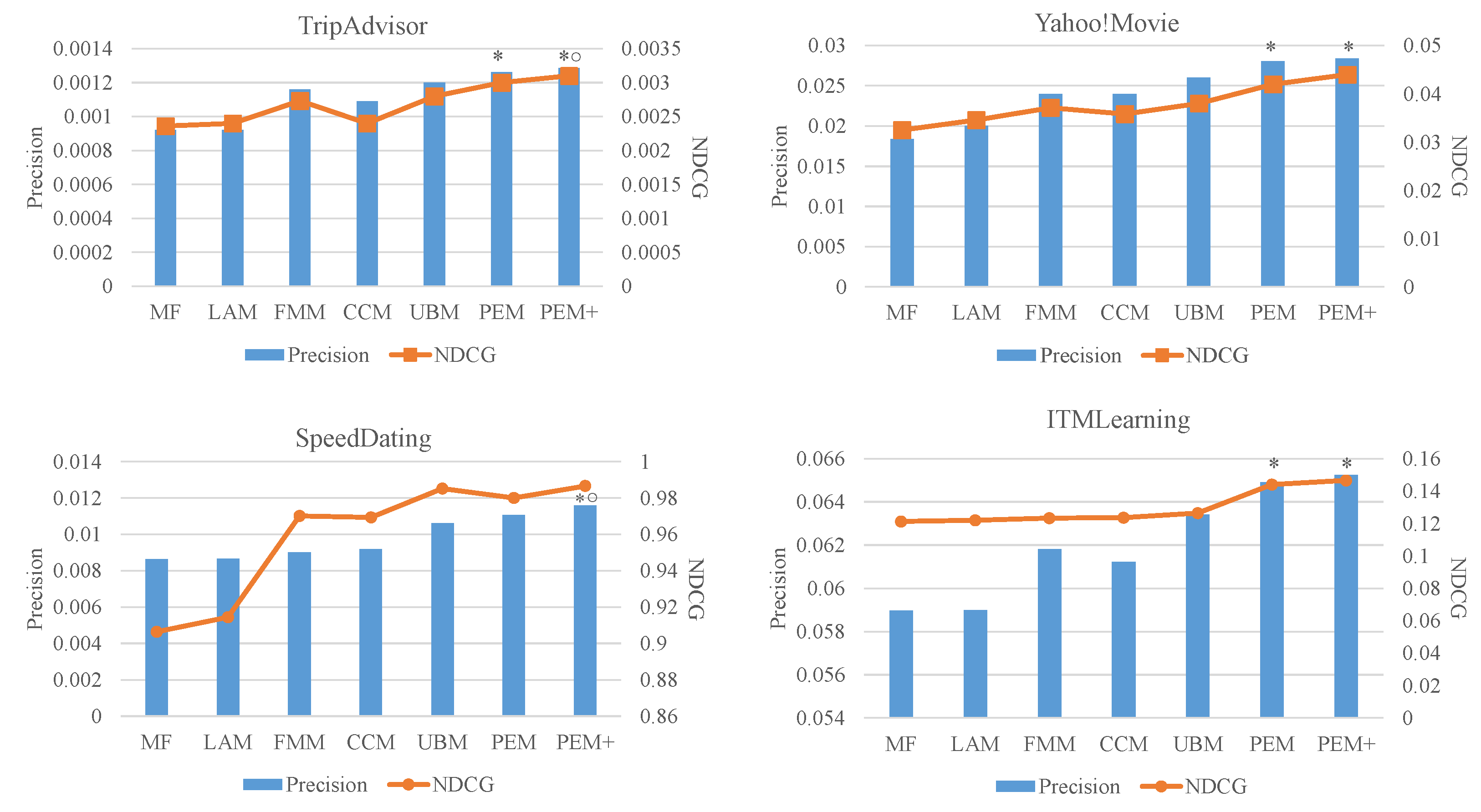
First of all, we present the results based on precision and NDCG in Figure 2. Table 3 presents the NDCG results for the utility-based recommendation models, as well as the improvement by PEM and PEM+ in comparison with UBM. We performed two-paired t-test as the significant test at the 95% confidence level. We use * to represent significant results between proposed approach (i.e., PEM and PEM+) and the best performing baseline method, and ∘ to indicate significant results between PEM and PEM+. Significance results based on precision are depicted in Figure 2, while the results for NDCG are described in Table 3.
First of all, we compared the results among the baseline methods (i.e., MF, LAM, FMM, CCM and UBM). We observed that the UBM approach generally outperformed other baseline methods in terms of both precision and NDCG. UBM produced slightly better NDCG results than the NDCG by FMM in the TripAdvisor and Yahoo!Movie data.
By comparing the solutions proposed in this paper (i.e., PEM and PEM+) with the baseline methods, we observed that the PEM could offer improvements on both precision and NDCG on all the data sets, except the speed dating data. PEM+ was able to beat all baselines except the speed dating data too. We believe that the failure was caused by the characteristics of this data set, which will be discussed in the next paragraph. A further look at the comparison between PEM and PEM+ can tell that PEM+ beat PEM in NDCG for all data except the dating data. However, PEM+ failed to outperform PEM in precision for the Yahoo!Movie and ITMLearning data. Recall that we used the NDCG as the fitness function in PSO, while the results on precision may be out of controls. Another potential reason could be that we did not try larger K values in KMeans for PEM+.
As a summary, PEM and PEM+ could offer improvements over the utility-based recommendation model. The only exception was the SpeedDating data set. We did have multi-criteria ratings in this data set. However, it was a data set for people-to-people recommendations which fell in the category of reciprocal recommendations. The nature of this data was different from other multi-criteria rating data, which may have resulted in less improvements here. We observed that the NDCG was even decreased by using PEM. The underlying reasons may lie in the special characteristics of the reciprocal recommendations. In the context of speed dating, a successful recommendation will consider a “match” between two users. In our recommendation approach, we only considered the preferences from the perspective of the users who received the recommendations, but ignored whether the recommended people would like to date with the target user. It may result in a drop or less improvements. A reciprocal recommendation model which also considers the dating partners [37,38] may help improve the recommendation performance.
Our previous research [8] proposed to use the filtering strategies to alleviate the issue of over-/under-expectations for the ITMLearning data. We chose the best filtering strategy and run the model. It achieved the NDCG result as 0.1311 which was lower than the results by using both PEM and PEM+. It is not surprising, since the filtering operation may mistakenly remove the items that a user may like. Our solution based on the penalties actually provided a soft and finer-grained solution to alleviate the issue of over-/under-expectations. These results demonstratde that our solution was much more effective than the filtering strategy, not to mention that the penalty-enhanced solution did not require any domain knowledge to define the rules for filtering.
Finally, we present the learned P o v e r and P u n d e r by using the PEM approach, as shown by Table 4.
We observed that the penalties learned by our models varied from case to case. The “penalty” was positive for over-expectations and negative for under-expectations for the TripAdvisor, Yahoo!Movie and ITMLearning data sets. It tells that the users still liked the item if it was over-expected, and additionally a bonus was added to the predicted score which was used to rank the items. The penalty was negative in the case of under-expectation, so the predicted score was penalized accordingly. The pattern in the SpeedDating data was different from others—the penalty for over-expectation was negative, while it was positive for under-expectations. It implies that a user may not have accepted a recommended partner if some characteristics of the partner were over-expected. By contrast, the penalty for under-expectation was positive but close to zero, which implies that a partner was still acceptable even if the partner slightly missed the expectations in some characteristics. These results are interesting and can also help us understand more characteristics about each data or domain.

6. Conclusions and Future Work

In this paper, we point out the issue of over-/under-expectations in the existing utility-based multi-criteria recommendation approach, and propose to learn penalties to alleviate this issue. Our experimental results based on four real-world data sets can demonstrate the effectiveness of the proposed solutions. Particularly, the penalty-enhanced approach works better than the filtering strategy, and it is general enough to be applied to any data sets.
However, there are still some limitations in the current work. We can consider more solutions for these issues as our future work. First of all, we define the case of over-/under-expectation for each rating entry by a user on an item, and apply the corresponding penalties. We can actually exploit a finer-grained method which will apply a penalty to each bit of the rating vector (i.e., case by case for the rating on each criterion). In this case, we have more penalties to be learned, but it may be able to further improve the models. In addition, we did not try larger K values for the KMeans clustering in the PEM+ method. Other K values may deliver better results. Using PSO as the optimizer may result in an efficiency issue for a large-scale data. We can use cloud service (such as Amazon Web Services) to learn the parameters. Or, we can seek other optimization methods in future. Finally, the penalties may be affected by other information, such as contexts [39,40] or trust information [41,42]. For example, the issue of over-/under-expectations may be serious in some contexts, but they can be ignored in other situations. Or, the issue can be ignored if the item was recommended by a trusted person. We will seek these alternative improvements in our future work.

Funding

This research received no external funding.

Conflicts of Interest

The author declares no conflict of interest.

Abbreviations

The following abbreviations are used in this manuscript:
CCMCriteria Chain Model
DCGDiscounted Cumulative Gain
FMMFlexible Mixture Model
LAMLinear Aggregation Model
MCRSMulti-Criteria Recommender Systems
MFMatrix Factorization
MOEAMulti-Objective Evolutionary Algorithms
NDCGNormalized Discounted Cumulative Gain
PEMPenalty-Enhanced Model
PSOParticle Swarm Optimization
UBMUtility-Based Model

References

  1. Bawden, D.; Robinson, L. The dark side of information: Overload, anxiety and other paradoxes and pathologies. J. Inf. Sci. 2009, 35, 180–191. [Google Scholar] [CrossRef]
  2. Alexandridis, G.; Siolas, G.; Stafylopatis, A. ParVecMF: A paragraph vector-based matrix factorization recommender system. arXiv 2017, arXiv:1706.07513. [Google Scholar]
  3. Alexandridis, G.; Tagaris, T.; Siolas, G.; Stafylopatis, A. From Free-text User Reviews to Product Recommendation using Paragraph Vectors and Matrix Factorization. In Companion Proceedings of the 2019 World Wide Web Conference; Association for Computing Machinery: New York, NY, USA, 2019; pp. 335–343. [Google Scholar]
  4. Adomavicius, G.; Kwon, Y. New recommendation techniques for multicriteria rating systems. IEEE Intell. Syst. 2007, 22, 48–55. [Google Scholar] [CrossRef] [Green Version]
  5. Zheng, Y. Utility-based multi-criteria recommender systems. In Proceedings of the 34th ACM/SIGAPP Symposium on Applied Computing, Limasso, Cyprus, 8–12 April 2019; pp. 2529–2531. [Google Scholar]
  6. Liu, T.Y. Learning to Rank for Information Retrieval; Springer Science & Business Media: Berlin/Heidelberg, Germany, 2011. [Google Scholar]
  7. Balakrishnan, S.; Chopra, S. Collaborative ranking. In Proceedings of the Fifth ACM International Conference on Web Search and Data Mining, Seattle, WA, USA, 8–12 February 2012; pp. 143–152. [Google Scholar]
  8. Zheng, Y.; Ghane, N.; Sabouri, M. Personalized Educational Learning with Multi-Stakeholder Optimizations. In Proceedings of the Adjunct ACM Conference on User Modelling, Adaptation and Personalization, Larnaca, Cyprus, 9–12 June 2019. [Google Scholar]
  9. Manouselis, N.; Costopoulou, C. Experimental analysis of design choices in multiattribute utility collaborative filtering. Int. J. Pattern Recognit. Artif. Intell. 2007, 21, 311–331. [Google Scholar] [CrossRef]
  10. Sahoo, N.; Krishnan, R.; Duncan, G.; Callan, J. Research Note—The Halo Effect in Multicomponent Ratings and Its Implications for Recommender Systems: The Case of Yahoo! Movies. Inf. Syst. Res. 2012, 23, 231–246. [Google Scholar] [CrossRef] [Green Version]
  11. Zheng, Y. Criteria Chains: A Novel Multi-Criteria Recommendation Approach. In Proceedings of the 22nd International Conference on Intelligent User Interfaces, Limassol, Cyprus, 13–16 March 2017; pp. 29–33. [Google Scholar]
  12. Burke, R. Hybrid recommender systems: Survey and experiments. User Model. User-Adapt. Interact. 2002, 12, 331–370. [Google Scholar] [CrossRef]
  13. Schafer, J.B.; Frankowski, D.; Herlocker, J.; Sen, S. Collaborative filtering recommender systems. In The Adaptive Web; Springer: Berlin/Heidelberg, Germany, 2007; pp. 291–324. [Google Scholar]
  14. Ekstrand, M.D.; Riedl, J.T.; Konstan, J.A. Collaborative Filtering Recommender Systems. Available online: https://dl.acm.org/doi/10.1561/1100000009 (accessed on 23 November 2020).
  15. Pazzani, M.J.; Billsus, D. Content-based recommendation systems. In The Adaptive Web; Springer: Berlin/Heidelberg, Germany, 2007; pp. 325–341. [Google Scholar]
  16. Lops, P.; De Gemmis, M.; Semeraro, G. Content-based recommender systems: State of the art and trends. In Recommender Systems Handbook; Springer: Berlin/Heidelberg, Germany, 2011; pp. 73–105. [Google Scholar]
  17. Zhao, W.X.; Li, S.; He, Y.; Wang, L.; Wen, J.R.; Li, X. Exploring demographic information in social media for product recommendation. Knowl. Inf. Syst. 2016, 49, 61–89. [Google Scholar] [CrossRef] [Green Version]
  18. Burke, R. Knowledge-based recommender systems. Encycl. Libr. Inf. Syst. 2000, 69, 175–186. [Google Scholar]
  19. Tarus, J.K.; Niu, Z.; Mustafa, G. Knowledge-based recommendation: A review of ontology-based recommender systems for e-learning. Artif. Intell. Rev. 2018, 50, 21–48. [Google Scholar] [CrossRef]
  20. Guttman, R.H. Merchant Differentiation through Integrative Negotiation in Agent-Mediated Electronic Commerce. Ph.D. Thesis, Massachusetts Institute of Technology, Cambridge, MA, USA, 1998. [Google Scholar]
  21. Zihayat, M.; Ayanso, A.; Zhao, X.; Davoudi, H.; An, A. A utility-based news recommendation system. Decis. Support Syst. 2019, 117, 14–27. [Google Scholar] [CrossRef]
  22. Li, Z.; Fang, X.; Bai, X.; Sheng, O.R.L. Utility-based link recommendation for online social networks. Manag. Sci. 2017, 63, 1938–1952. [Google Scholar] [CrossRef] [Green Version]
  23. Ribeiro, M.T.; Lacerda, A.; Veloso, A.; Ziviani, N. Pareto-efficient hybridization for multi-objective recommender systems. In Proceedings of the Sixth ACM Conference on Recommender Systems, Dublin, Ireland, 9–13 September 2012. [Google Scholar]
  24. Ribeiro, M.T.; Ziviani, N.; Moura, E.S.D.; Hata, I.; Lacerda, A.; Veloso, A. Multiobjective pareto-efficient approaches for recommender systems. ACM Trans. Intell. Syst. Technol. 2014, 5, 1–20. [Google Scholar]
  25. Koren, Y.; Bell, R.; Volinsky, C. Matrix factorization techniques for recommender systems. Computer 2009, 42, 30–37. [Google Scholar] [CrossRef]
  26. Valizadegan, H.; Jin, R.; Zhang, R.; Mao, J. Learning to Rank by Optimizing NDCG Measure. Available online: https://dl.acm.org/doi/10.5555/2984093.2984304 (accessed on 23 November 2020).
  27. Donmez, P.; Svore, K.M.; Burges, C.J. On the local optimality of LambdaRank. In Proceedings of the 32nd International ACM SIGIR Conference on Research and Development in Information Retrieval, Boston, MA, USA, 19–23 July 2009; pp. 460–467. [Google Scholar]
  28. Yeh, J.Y.; Lin, J.Y.; Ke, H.R.; Yang, W.P. Learning to rank for information retrieval using genetic programming. In Proceedings of the SIGIR 2007 Workshop on Learning to Rank for Information Retrieval (LR4IR 2007), Amsterdam, The Netherlands, 23–27 July 2007. [Google Scholar]
  29. Ujjin, S.; Bentley, P.J. Particle swarm optimization recommender system. In Proceedings of the 2003 IEEE Swarm Intelligence Symposium, SIS’03 (Cat. No. 03EX706), Indianapolis, IN, USA, 26 April 2003; pp. 124–131. [Google Scholar]
  30. Zheng, Y.; Burke, R.; Mobasher, B. Recommendation with differential context weighting. In Proceedings of the International Conference on User Modeling, Adaptation, and Personalization, Rome, Italy, 10–14 June 2013; Springer: Berlin/Heidelberg, Germany, 2013; pp. 152–164. [Google Scholar]
  31. Poli, R.; Kennedy, J.; Blackwell, T. Particle swarm optimization. Swarm Intell. 2007, 1, 33–57. [Google Scholar] [CrossRef]
  32. Kanungo, T.; Mount, D.M.; Netanyahu, N.S.; Piatko, C.D.; Silverman, R.; Wu, A.Y. An efficient k-means clustering algorithm: Analysis and implementation. IEEE Trans. Pattern Anal. Mach. Intell. 2002, 24, 881–892. [Google Scholar] [CrossRef]
  33. Jannach, D.; Zanker, M.; Fuchs, M. Leveraging multi-criteria customer feedback for satisfaction analysis and improved recommendations. Inf. Technol. Tour. 2014, 14, 119–149. [Google Scholar] [CrossRef]
  34. Zheng, Y. Personality-Aware Decision Making In Educational Learning. In Proceedings of the 23rd International Conference on Intelligent User Interfaces, Tokyo, Japan, 7–11 March 2018; p. 58. [Google Scholar]
  35. Shi, Y.; Eberhart, R.C. Empirical study of particle swarm optimization. In Proceedings of the 1999 Congress on Evolutionary Computation-CEC99, Washington, DC, USA, 6–9 July 1999; Volume 3, pp. 1945–1950. [Google Scholar]
  36. Sierra, M.R.; Coello, C.A.C. Improving PSO-based multi-objective optimization using crowding, mutation and ϵ-dominance. In Proceedings of the International Conference on Evolutionary Multi-Criterion Optimization, Guanajuato, Mexico, 9–11 March 2005; Springer: Berlin/Heidelberg, Germany, 2005; pp. 505–519. [Google Scholar]
  37. Pizzato, L.; Rej, T.; Chung, T.; Koprinska, I.; Kay, J. RECON: A reciprocal recommender for online dating. In Proceedings of the Fourth ACM Conference on Recommender Systems, Barcelona, Spain, 26–30 September 2010; pp. 207–214. [Google Scholar]
  38. Zheng, Y.; Dave, T.; Mishra, N.; Kumar, H. Fairness In Reciprocal Recommendations: A Speed-Dating Study. In Proceedings of the Adjunct ACM Conference on User Modelling, Adaptation and Personalization, Singapore, 8–11 July 2018. [Google Scholar]
  39. Adomavicius, G.; Mobasher, B.; Ricci, F.; Tuzhilin, A. Context-Aware Recommender Systems. AI Mag. 2011, 32, 67–80. [Google Scholar] [CrossRef]
  40. Adomavicius, G.; Tuzhilin, A. Context-aware recommender systems. In Recommender Systems Handbook; Springer: Berlin/Heidelberg, Germany, 2011; pp. 217–253. [Google Scholar]
  41. Agreste, S.; De Meo, P.; Ferrara, E.; Piccolo, S.; Provetti, A. Trust networks: Topology, dynamics, and measurements. IEEE Internet Comput. 2015, 19, 26–35. [Google Scholar] [CrossRef]
  42. Lee, J.; Noh, G.; Oh, H.; Kim, C.k. Trustor clustering with an improved recommender system based on social relationships. Inf. Syst. 2018, 77, 118–128. [Google Scholar] [CrossRef]
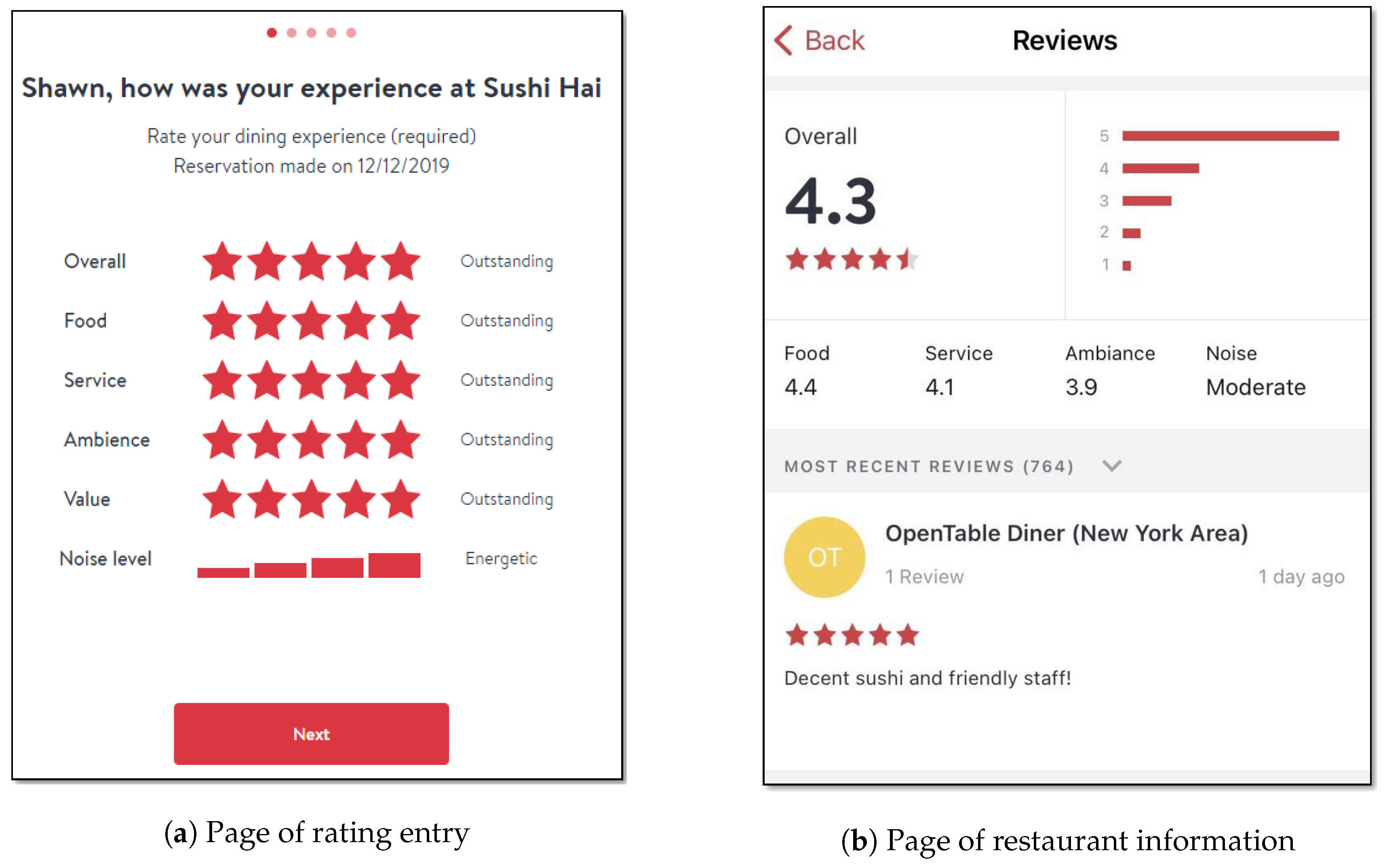
Figure 1. Example of user preferences on multiple criteria.
Information 11 00551 g001
Figure 2. Experimental results.
Information 11 00551 g002
Table 1. Example of Rating Matrix from OpenTable.
UserItemRatingFoodServiceValue
U 1 T 3 4434
U 2 T 2 3333
U 3 T 1 ????
Table 2. Example of over-/under-expectation.
UserItemFoodServiceValueAmbiance
u T 1 2222
u T 2 4444
u T 3 1421
u’s expectation3333
Table 3. Results based on normalized discounted cumulative gain (NDCG).
TripAdvisorYahoo!MovieSpeedDatingITMLearning
UBM0.00280.0380.98520.1264
PEM0.003 (7.14%)
*
0.042 (10.5%)
*
0.98 (−0.5%)0.1441 (14%)
*
PEM+0.0031 (10.7%)
* ∘
0.044 (15.8%)
* ∘
0.9866 (0.14%)0.1466 (15.9%)
* ∘
Table 4. Learned penalties.
P over P under
TripAdvisor0.124−0.022
Yahoo!Movie0.574−0.985
SpeedDating−0.290.02
ITMLearning0.324−0.165
Publisher’s Note: MDPI stays neutral with regard to jurisdictional claims in published maps and institutional affiliations.