Abstract
An efficient and credible approach to road traffic management and prediction is a crucial aspect in the Intelligent Transportation Systems (ITS). It can strongly influence the development of road structures and projects. It is also essential for route planning and traffic regulations. In this paper, we propose a hybrid model that combines extreme learning machine (ELM) and ensemble-based techniques to predict the future hourly traffic of a road section in Tangier, a city in the north of Morocco. The model was applied to a real-world historical data set extracted from fixed sensors over a 5-years period. Our approach is based on a type of Single hidden Layer Feed-forward Neural Network (SLFN) known for being a high-speed machine learning algorithm. The model was, then, compared to other well-known algorithms in the prediction literature. Experimental results demonstrated that, according to the most commonly used criteria of error measurements (RMSE, MAE, and MAPE), our model is performing better in terms of prediction accuracy. The use of Akaike’s Information Criterion technique (AIC) has also shown that the proposed model has a higher performance.
1. Introduction
The growing size of cities and increasing population mobility have caused a rapid increase in the number of vehicles on the roads. Road traffic management now faces such challenges as traffic congestion, accidents, and air pollution. Recent statistics reveal that the majority of vehicle crashes usually happen in the areas around congested roads. This is due to the fact that the drivers tend to drive faster, before or after encountering congestions, in order to compensate for the experienced delay. As a consequence, researchers from both industry and academia focused on making traffic management systems (TMS) more efficient to cope with the above issues. Traffic data are growing fast, and their analysis is a key component in developing a road network strategy. The most important question is how to analyze and benefit from this gold mine of information in order to bring out predictions of future data. An accurate traffic prediction system is one of the critical steps in the operations of an Intelligent Transportation System (ITS) and is extremely important for practitioners to perform route planning and traffic regulations.
In this context, the primary motivation of this work is to exploit the mass of historical information collected from a road section in order to predict the next hourly traffic. The fundamental challenge of road safety is predicting the possible future states of road traffic with pinpoint accuracy. Predicted information helps to prevent the occurrence of such incidents as congestion or other road anomalies [1]. Moreover, the prediction of traffic flow can eventually contribute to anticipating operations to improve road infrastructures.
The literature often refers to traffic as a flow, because it has similar properties to fluids. Thus, when we speak about traffic flow prediction, we wish to predict the next state (volume, speed, density, or behavior) of the traffic flow based on historical and/or real-time data. Prediction or forecasting is the essence of intelligent systems and is vital in the decision-making process.
Researchers have paid great attention to this field because of its importance. They have considered many suitable methods starting from traffic models to statistical or machine learning approaches. Predictive analytics rely on a variety of analytical techniques, including predictive modeling and data mining [2]. They use both historical and current statistics to estimate, or ‘predict’ future outcomes [3].
Machine learning is a subfield of artificial intelligence that evolved from the study of pattern recognition to explore the notion that algorithms can learn from and make predictions on data. Moreover, as they begin to become more ‘intelligent’, these algorithms can overcome program instructions to produce highly accurate and data-driven decisions. There are three types of machine learning algorithms: supervised learning (regression, decision tree, KNN, logistic regression, etc.), Unsupervised Learning (Apriori algorithm, K-means…) and Reinforcement Learning (Markov Decision Process-learning…) [4]. Machine learning algorithms are widely used in addressing various problems in different fields including medicine applications [5,6].
Heuristics based on a statistical analysis of historical data are easy and practical for prediction, like the KNN algorithm, linear and nonlinear regression, and autoregressive linear models such as Autoregressive Integrated Moving Average (ARIMA) [7,8,9]. In statistical techniques, ARIMA models are, in theory, the most general class of models to forecast time series data. They can potentially and effectively predict future data because of their convenience and accurate prediction, low data input requirement, and simple computation [10,11]. However, ARIMA methods need to convert the input time series to a stationary series. On the other hand, the underlying process used in the ARIMA model is linear, thus failing to capture nonlinear models from the time series [1]. For regression problems, the Support Vector Regression (SVR) model has proved to be a powerful tool in real data estimation [12]. As a supervised learning algorithm in machine learning, the SVR model uses symmetric loss function, which penalizes boundary decisions. There is, however, no theory on how to choose proper kernel function in a data-dependent way. It is also slower than other artificial neural networks (ANN) for similar generalization performance. Recently, ANN has grabbed a lot of attention in this area. Historical events such as school-timings, holidays, and other periodic events are utilized to predict the traffic volume based on the historical data in each major junction in the city using ANN [13]. ELM, a novel learning algorithm for Single hidden Layer Feed-forward Neural Network (SLFN), was recently proposed as a unifying framework for different families of learning algorithms. ELM not only has a simple structure but also learns faster with better generalization performance. A framework based on Exponential Smoothing and extreme learning machine for the prediction of road traffic is proposed in [14]. The Taguchi method was used for the optimization of the parameters of the model, which performed well in terms of efficiency and high precision. ELM technique is also used in [15] to predict real-time traffic data with high accuracy. Some researchers also considered this technique to forecast the flow congestion on a single road section [16]. Afterward, their approach allows the prediction of congestion on all the roads of the city. Authors of [17] proposed on-line sequential extreme learning machine for short-term prediction of road traffic. Their approach showed high performance comparing to the ELM model; however, it requires a large number of neurons, a large dataset and does not take into account factors that can influence road traffic. More research work applied ELM to improve the short-term prediction, but they did not consider overcoming the problem and/or minimizing the fluctuations generated by ELM [18].
Researchers have also tried several deep neural network configurations to forecast traffic flow [19,20,21,22]. In [19], the methodology used to predict traffic flows during special events showed how deep learning provides precise short-term traffic flow predictions. However, these are time-consuming and require a large number of traffic data. Some scientists considered the hybrid schemes that combine different models to forecast the traffic, pointing out that single models are not efficient enough to handle all kinds of traffic situations [23]. While these models have various levels of success, complex ones are time-consuming and not simple to implement.
In this study, we propose a hybrid model that combines extreme learning machine (ELM) and ensemble-based techniques for road traffic prediction. Compared with traditional neural networks and support vector machine, ELM offers significant advantages such as fast learning speed, ease of implementation, and minimal human intervention [24,25]. We conducted a comparative study with traditional learning algorithms (MLP, SVR and ARIMA) and concluded that our model is higher performing in terms of prediction accuracy. The experiment’s results showed that our system is robust to the outliers and has superior generalization capability.
The sources of data utilized are extracted from sensors in fixed positions, which were able to detect the presence of nearby vehicles. Initially, inductive loop detectors were the most popular, but nowadays, a wide variety of sensors have become available [26]. The set of data recorded consists of the number of vehicles passing through a road section together with the parameter of date and time information. It covers a 5-year period from 2013 to 2017. The road section considered is about 13 km and is located in Tangier, a major city of northern Morocco. It is located on a bay facing the Strait of Gibraltar 17 miles (27 km) from the southern tip of Spain. It links the continent to Europe through its port and connects the city to the rest of the country.
This paper attempts to provide satisfying answers to the following questions:
- What are the necessary features for road traffic prediction?
- How can we build a dataset based on fixed sensing data?
- How can we process our dataset using machine learning algorithms?
- How can we improve the predictability of our model?
The rest of the paper is organized as follows:
2. Methodology and the Proposed Approach
This section is dedicated to present the proposed methodology and the process of building the dataset that will be used for our study.
2.1. Data Collection
The source of data was obtained from The Moroccan center for road studies and research. The analysis of traffic data is an essential and critical indicator of the country’s infrastructure and transport system strategies. The center uses either permanent or temporary inductive loops embedded under the road surface to collect a massive amount of statistics about traffic flow in some of the major roads in Morocco. The dataset contains recorded traffic flow over a 5-years period from 2013 to 2017 and is composed of a set of separate files. Each file contains traffic information about a specific time-period. The meta-data of the files includes the date (day and hour) of the start and end of the recording, number of lanes, and also traffic decomposition by the class of the vehicle based on their length L (Table 1 and Table 2).

Table 1.
Sample data from a generated file for a two-lane road with vehicle classes.
Table 2.
Vehicle classification based on their length (L).
2.2. Data Preprocessing
The first step in the process of building the dataset consists of merging the road traffic data in a single file. In our study, we will consider the sum of hourly traffic for all classes of vehicles. Data is then preprocessed by first adding some appropriate features that may influence the type of traffic flow and that constitute the input layer of our model (Figure 1):
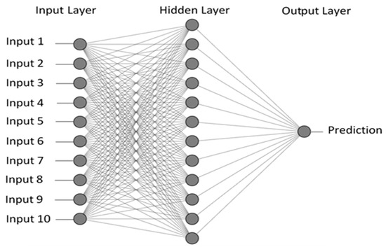
Figure 1.
Structure of ELM model.
- Feature 1: Day of the week (Monday, Tuesday, Wednesday…)
- Feature 2: Type of holiday (national, religious or other)
- Feature 3: Part of the day (morning or evening)
- Feature 4: Schooling/vacation/public holiday
- Feature 5: Last hourly traffic (hour-1)
- Feature 6: Observation of the previous day the same hour (day-1)
- Feature 7: Last Week observation for same day and same hour (week-1)
- Feature 8: Last month observation for same day and same hour(month-1)
- Feature 9: Hour observation (traffic flow all type of vehicles)
- Feature 10 (*): Time slot (7 periods)
(*): The day is divided into different periods that have seemingly different classes of traffic: 01:00–05:59, 06:00–8:59, 09:00–10:59, 11:00–14:59, 15:00–17:59, 18:00–21:59 and 22:00–00:59.
The second step is to remove the data records that have missing values because some observations may be lacking due to sensor failure or absence of some features data. The next step of data preprocessing is data standardization. By standardizing the data, all data values will fall within a given range, and the incidence of input factors can be assessed based on the pattern shown by the input factors, but not on the numeric magnitude. Data standardization has two main advantages: It reduces the scale of the network and ensures that input factors with large numerical values do not eclipse those with smaller numerical values. Machine learning algorithms may be affected by data distribution. Thus, the model might finish with reduced accuracy. Given the use of small weights in the model, and the error between the predicted and expected values, the scale of inputs and outputs used to train the model is a crucial factor. Unscaled input variables may result in a slow or unstable learning process, while unscaled target variables on regression problems may result in an exploding gradient causing the failure of the learning process. So, it is highly recommended to rescale data in the same range to eliminate a multi-range of features.
One of the techniques that permit scaling data is the Min-Max normalization; the default range of scaling is 0 to 1.
The Features Data was normalized using the previous formula, i.e., the default range scaling. Target Data was normalized in [−1, 1] range given by the equation:
where a and b represent respectively the min and the max range that are in our case, respectively, −1 and 1.
2.3. Methods
2.3.1. Extreme Learning Machine
The extreme learning machine (ELM) is a novel and fast learning method for SLFNs (Figure 2), where the inputs weights and the hidden layer biases are randomly chosen [24]. The optimization problem arising in learning the parameters of an ELM model can be solved analytically, resulting in a closed-form involving only matrix multiplication and inversion [27]. Hence, the learning process can be carried out efficiently without requiring an iterative algorithm, such as a backpropagation-neural network (BP-NN), or the solution to a quadratic programming problem as in the standard formulation of SVM. In ELM, the input weights (linking the input layer to the hidden layer) and hidden biases are randomly chosen, and the output weights (linking the hidden layer to the output layer) are analytically determined by using Moore-Penrose MP generalized inverse [28].
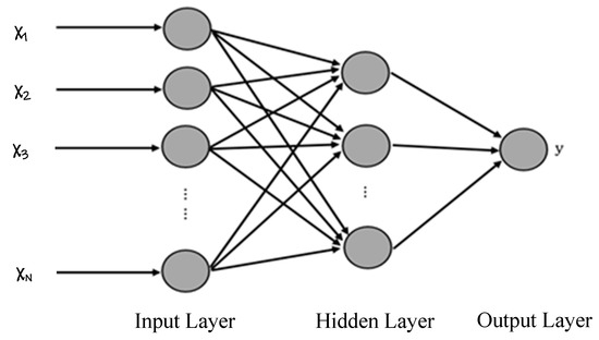
Figure 2.
Structure of SLFN.
Given a finite training set, represent the input variables and represent the output variables. The SLFN neural Network with N hidden layer neurons is written in the following general form:
where is the input weight vector of the ith hidden layer neuron. is the output weight vector of the ith hidden layer neuron. is the threshold of the ith hidden layer neuron, and g(x) is the activation function.
ELM search to minimize training error:
Which is equivalent to:
The above equations can be written:
H is the output matrix of the hidden layer:
The output matrix is calculated by:
where is the Moore–Penrose generalized inverse of H.
2.3.2. Ensemble Based Systems in Decision Making
Ensemble Based System in Decision Making (EBDM) is a process that uses a set of models, each of them obtained by applying a machine learning technic to specific data. EBDM then integrates these models each of them differently in order to get the final prediction. They have been widely used in machine learning and pattern recognition applications since they have demonstrated to perform favorably and significantly increase prediction accuracy as compared to single models. There are many reasons to use EBDM, including statistics, the large volume of data, too little data, or data fusion. More details are available in [29]. There are several technics, including methods that use a combination of rules such as algebraic combination; voting-based approach; decision templates; and methods based on neural networks such as Bagging, Boosting, and AdaBoost that require modifications to the learning process [30]. The technique adopted in this paper is Arithmetic Averaging because it is simple and allows having powerful results [2]. The general formula is:
where N is the number of ensembles, is the output of the ith time and is the average output to be considered.
The ELM model generates different values for each application on the test dataset due to the random generation of its input weights and the bias of the hidden layer. However, these variations in predictions are negligible compared to those of other ANNs. Still, to solve this issue, we will consider the ensemble methods that are used to reduce these small fluctuations and make the prediction more robust than the simple model with better precision. To do this, we will get several ELM models that we will apply to our data while keeping the test and training datasets the same. Since the prediction results are different for each model, the final predicted value considered will be the algebraic mean of all the results obtained.
2.3.3. Autoregressive Integrated Moving Average (ARIMA)
The ARIMA model for Autoregressive Integrated Moving Average has been used extensively in time series modeling as it is robust and easy to implement. The auto regression (AR) part of ARIMA is a linear regression on the prior values of the variable of interest and can predict future values. The moving average (MA) part is also a linear regression of the past forecast residual errors. The I in ARIMA stands for integrated and refers to the differencing by computing the differences between consecutive observations to eliminate the non-stationarity. The full ARIMA (p, d, q) model can be written as:
To determine the values of p and q, one can use the autocorrelation function (ACF) and partial autocorrelation function (PACF) plots. The ACF plot shows the autocorrelation between y’t and y’t−k, and the PACF shows the autocorrelations between y’t and y’t−k after removing the effects of lags 1, 2, 3, …, k−1.
2.3.4. Support Vector Regression
Support Vector Regression (SVR) is a regression algorithm, and it applies a similar technique of support vector machines (SVM) for regression analysis. As we know, regression data contains continuous real numbers. To model such type of data, the SVR model fits the regression line in a way that it approximates the best values with a given margin called ε-tube (epsilon-tube ε identifies a tube width). SVR attempts to fit the hyperplane that has a maximum number of points while minimizing the error. The ε-tube takes into consideration the model complexity and error rate, which is the difference between actual and predicted outputs. The constraints of the SVR problem are described as:
where the equation of the hyperplane is:
The objective function of SVR is to minimize the coefficients:
2.3.5. Multi-Layer Perceptron
Multi-layer Perceptron (MLP) is a type of feedforward neural network (FNN) that uses a supervised learning algorithm. It can learn a non-linear function approximator for either classification or regression. The simplest MLP consists of three or more layers of nodes: an input layer, a hidden layer and an output layer. It has the following disadvantages: MLP requires tuning a number of hyperparameters such as the number of hidden neurons, layers, and iterations. Moreover, MLP is sensitive to feature scaling.
For regression problem, MLP use backpropagation (BP) to calculate gradients to minimize the square error loss function. Since BP has a high computational complexity, it is advisable to start with a smaller number of hidden neurons and few hidden layers for training. However, if it has few (in contrast to large) neurons, it might have a high training error due to underfitting (in contrast to overfitting). Therefore, BP-based ANNs tend to exhibit sub-optimal generalization performance [24,31].
3. Data Processing and Experimental Results
3.1. Evaluation Metrics
The model built may be evaluated by different criteria; it gives us a clear view of its performance and how well it correctly predicts the results. For regression models that predict numerical values, there are several metrics, such as RMSE, MAE, and MAPE [32]. In this paper, the three previous Metrics were used to evaluate model accuracy. In addition to these three indices, the AIC has been used to perform model comparisons. The formulas of these indices are given as follows:
RMSE: the formula calculates Root Mean Square Error:
MAE: Mean Absolute Error’s formula is:
MAPE: Mean Absolute Percentage Error is given by:
where N represents the number of observations in the test dataset, is the reel output of ith observation and is the predicted value for ith observation.
AIC: The Akaike’s Information Criterion [33] is used to check the complexity of models. The model with minimum AIC value is considered as the best and less complex among alternative models. The AIC formula is defined by:
where RSS is the Residual Sum of Squares, K is the total number of parameters in the model, and n is the number of observations.
3.2. Proposed Framework and Prediction Evaluation of ELM Model
In order to reduce the fluctuations generated by the ELM model, we have considered ensemble methods. The purpose is to make the final decision of the model more accurate. The proposed framework combines the high performance of ELM with the advantages of ensemble methods. In the first step, we fit N times the ELM model on our training data, where N is the number of ensembles. The choice of the number of neurons in the hidden layer of ELM, as well as N, is made based on the quality of the results. Subsequently, the outputs of the ensemble are algebraically combined by averaging, which can reduce the risk of bad selection of a poor predictor (Figure 3).
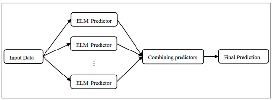
Figure 3.
Proposed Framework of traffic prediction using ensemble method.
It is generally known that several parameters may influence the accuracy of the model, such as the number of hidden neurons, the size of the data, and the used activation function. Various researchers and specialists in this field generally test several combinations or use approved approaches. The ELM algorithm may give different results for diverse parameters. Therefore, we have considered 20, 50, and 100 trials for each fixed size of the ELM model, and the result taken into account is the average result values. Our ELM network is composed of 10 input layer neurons (attributes), a hidden layer, and a single node of the output layer giving the 1 h traffic prediction. The choice of the size of the hidden layer is based on the results of several tests; the number of neurons giving the best performance is then considered.
Figure 4a illustrates the average test error RMSE. As shown in the figure, the outputs are normalized between 0 and 1; it represents the traffic test set RMSE. After 10 tests, we find out that the optimal number of hidden nodes for our learning set varies between 80 and 360, as described by [24]. We observe that RMSE decreases as the number of neurons increases, and that is optimized at 180 neurons in the hidden layer. Due to the random selection of hidden neurons, these results are given by several trials, and the average value is taken.
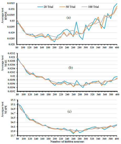
Figure 4.
Evolution of average errors in ELM model by changing the number of trials.
During the preparation of our dataset, it was decided to add information on features that better describe the observations (see Section 2.2). This resulted in incomplete records due to the absence of this information, representing a rate of 2.8% of the dataset size. Therefore, these records will not be considered and our model uses then 25,323 observations of which 22,790 are allocated to the learning phase and 2533 to test the model.
Then, the objective was to determine the optimal parameters for our model, namely the number of hidden neurons and the number of ensembles by considering the evaluation criteria that show less fluctuation.
The ELM algorithm was then evaluated several times to determine the best number of hidden neurons N. For this purpose, the model is tested on different sizes of the hidden layer in the range of 10 to 400 with a step of 10. For each hidden layer size, the model was trained, tested and evaluated successively 20 times, 50 times and 100 times. Evaluations criteria (RMSE, MAE and MAPE) are then calculated, and their average values are taken. Results of evaluation metrics of each number of trials are presented in Figure 4. It can be observed in the figure that the curves for the number of trials 50 and 100 have almost the same pattern with less fluctuation, which means that they have nearly the same quality of results.
Furthermore, the pattern of 20 trials shows some fluctuations that appear for the RMSE and MAE measurements, which mean that it will not probably be considered as the number of ensembles. On the other hand, the execution time of 50 trials is significantly faster than 100 trials. Consequently, the number of ensembles that will be considered in this study is actually 50.
The results of the evolution of the model performance according to the number of hidden neurons for 50 trials (Figure 4b,c) shows that for our training set, the optimal number of hidden neurons that have better results and less fluctuations is 250 neurons.
The simulation results were obtained using a 2.5 GHz Intel Core i5-7200U computer using Python 3.6.
3.3. Model Evaluation and Comparison to Other Methods
We tested the ELM model based on the obtained optimal number of neurons in the hidden layer. The performance of our model has been compared to SVR and ARIMA. We have tested several combinations of the cost parameter C and the kernel parameter. Authors of [30] recommend choosing the best combination among the values: and based on the cross-validation method.
In Figure 5, the x-axis represents the predicted hourly road traffic in chronological order. The y-axis describes the residues of the predicted values in relation to the real ones. We observe that there is no particular pattern for the five models; this actually proves a good fit. The shapes of the curves show that the hybrid EBDM model gives a remarkable improvement over the single ELM model. Moreover, the residues of this latter are clustered close to the line of equation 0. These smaller values indicate that our model is more accurate. This is definitely due to the right choice of relevant parameters as features, high quality of data after preprocessing, and number of neurons.
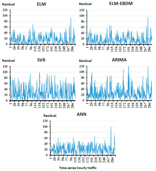
Figure 5.
The absolute residual error in test phase.
Figure 6 and Table 3 show that our model using EBDM generates better values with high accuracy than ELM itself. The y-axis represents the real value, the predicted one and the residues of the predicted values in relation to the real ones. It can be seen that fluctuations generated by random generalization of input parameters can be reduced. The EBDM actually reduces the prediction error of ELM while maintaining an acceptable execution time. This is thanks to the advantage of EBDM to adapt to small fluctuations generated by ELM at each prediction.
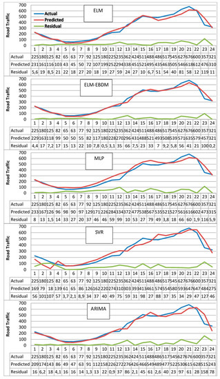
Figure 6.
Traffic prediction results of different models.
Table 3.
Prediction performance comparison by AIC, RMSE, MAE, and MAPE (*).
The Akaike Information Criterion (AIC) index takes into account the complexity and performance of the model; according to AIC values in Table 3, the EBDM model has the lowest costs in training phase. This confirms that our approach has superior quality than SVR, ARIMA and ANN models. As we can see in Figure 6 (ELM-EBDM), the hybrid model tries to reduce the fluctuations generated by the ELM model, which results in an improvement of the quality of the prediction results.
4. Conclusions
In this paper, we have discussed and employed the extreme learning machine algorithm to design an accurate model to predict hourly road traffic data. The study uses historical data from the past 5 years on a road section in Tangier, Morocco. The main contribution of our work is the development of a hybrid model called ELM-EBDM that shows far better performance than single ELM without affecting the speed of the learning process. Our proposed model has been evaluated by the comparison with the well-known algorithms MLP, SVR and ARIMA. The simulation results demonstrated that it gave a better performance in terms of both accuracy and stability. The proposed traffic prediction model represents a reliable tool for engineers and managers to plan roads and regulate traffic. It will also allow road users to have prior information about traffic to plan trips and manage time efficiently by avoiding the congestion hours.
The loop detectors used may know some malfunctions or a power failure, which can lead to incorrect or incomplete recordings. Therefore, our model will also serve to reconstitute lost or destroyed data with the predicted values. This allows filling in the gaps in the traffic matrix used to calculate the common traffic indicator Annual Average Daily Traffic (AADT). This indicator is widely considered for determining the type of road maintenance operations to be planned in the future
In our future work, we may consider some improvements through adding more relevant information about traffic. This includes specific events or weather conditions. Many adjacent roads and their traffic attributes may influence one particular road. Therefore, we will consider different numbers of nearby highways and traffic attributes for target roads to further improve the performance of our approach. We also plan to develop an algorithm to automatically determine the parameters: number of neurons and ensembles, as an alternative to the tedious manual selection method.
Author Contributions
Conceptualization, M.J. and A.M.; Methodology, M.J.; Software, A.M.; Validation, A.Y. and M.A.S.; Formal Analysis, A.Y., M.A.S. and J.B.; Investigation, M.J. and A.M.; Resources, M.J.; Data Curation, M.J. and A.M.; Writing Original Draft Preparation, M.J. and A.M.; Writing Review & Editing, M.J.; Visualization, M.J. and A.M.; Supervision, A.Y., M.A.S. and J.B. All authors have read and agreed to the published version of the manuscript.
Funding
This research received no external funding.
Acknowledgments
This research paper would not have been possible without the support and help of the national center for road studies and research CNER (Centre National d’Etudes et de Recherches Routières), which is attached to the ministry of equipment, transport, logistics, and water, of Morocco. The center spared no effort to share with us the process they follow to manage the road traffic and provided us with the necessary real traffic data that we have used in our research.
Conflicts of Interest
The authors declare no conflict of interest.
References
- Nagy, A.M.; Simon, V. Survey on traffic prediction in smart cities. Pervasive Mob. Comput. 2018, 50, 148–163. [Google Scholar] [CrossRef]
- Luo, D.; Chen, K. A Comparative Study of Statistical Ensemble Methods on Mismatch Conditions. In Proceedings of the 2002 International Joint Conference on Neural Networks, IJCNN’02 (Cat. No.02CH37290), Honolulu, HI, USA, 12–17 May 2002; Volume 1, pp. 59–64. [Google Scholar] [CrossRef]
- Jain, V.K.; Kumar, A.; Poonia, P. Short Term Traffic Flow Prediction Methodologies: A Review. Mody Univ. Int. J. Comput. Eng. Res. 2018, 2, 37–39. [Google Scholar]
- Tahifa, M.; Boumhidi, J.; Yahyaouy, A. Multi-agent reinforcement learning-based approach for controlling signals through adaptation. Int. J. Auton. Adapt. Commun. Syst. 2018, 11, 129. [Google Scholar] [CrossRef]
- D’Angelo, G.; Pilla, R.; Dean, J.B.; Rampone, S. Toward a soft computing-based correlation between oxygen toxicity seizures and hyperoxic hyperpnea. Soft Comput. 2018, 22, 2421–2427. [Google Scholar] [CrossRef]
- D’Angelo, G.; Pilla, R.; Tascini, C.; Rampone, S. A proposal for distinguishing between bacterial and viral meningitis using genetic programming and decision trees. Soft Comput. 2019, 23, 11775–11791. [Google Scholar] [CrossRef]
- Zhang, Y.; Liu, Y. Comparison of parametric and nonparametric techniques for non-peak traffic forecasting. World Acad. Sci. Eng. Technol. 2009, 39, 242–248. [Google Scholar]
- Kumar, S.V.; Vanajakshi, L. Short-term traffic flow prediction using seasonal ARIMA model with limited input data. Eur. Transp. Res. Rev. 2015, 7, 21. [Google Scholar] [CrossRef]
- Williams, B.M.; Hoel, L.A. Modeling and Forecasting Vehicular Traffic Flow as a Seasonal ARIMA Process: Theoretical Basis and Empirical Results. J. Transp. Eng. 2003, 129, 664–672. [Google Scholar] [CrossRef]
- Moeeni, H.; Bonakdari, H. Impact of Normalization and Input on ARMAX-ANN Model Performance in Suspended Sediment Load Prediction. Water Resour. Manag. 2018, 32, 845–863. [Google Scholar] [CrossRef]
- Moeeni, H.; Bonakdari, H. Forecasting monthly inflow with extreme seasonal variation using the hybrid SARIMA-ANN model. Stoch. Environ. Res. Risk Assess. 2017, 31, 1997–2010. [Google Scholar] [CrossRef]
- Awad, M.; Khanna, R.; Awad, M.; Khanna, R. Support Vector Regression. In Efficient Learning Machines; Apress: Berkeley, CA, USA, 2015; pp. 67–80. [Google Scholar]
- Çetiner, B.G.; Sari, M.; Borat, O. A Neural Network Based Traffic-Flow Prediction Model. Math. Comput. Appl. 2010, 15, 269–278. [Google Scholar] [CrossRef]
- Yang, H.-F.; Dillon, T.; Chang, E.; Chen, Y.-P.P. Optimized Configuration of Exponential Smoothing and Extreme Learning Machine for Traffic Flow Forecasting. IEEE Trans. Ind. Inform. 2019, 15, 23–34. [Google Scholar] [CrossRef]
- Chiang, N.-V.; Tam, L.-M.; Lai, K.-H.; Wong, K.-I.; Tou, W.-M.S. Floating Car Data-Based Real-Time Road Traffic Prediction System and Its Application in Macau Grand Prix Event. In Intelligent Transport Systems for Everyone’s Mobility; Springer: Singapore, 2019; pp. 377–392. [Google Scholar]
- Xing, Y.; Ban, X.; Liu, X.; Shen, Q. Large-scale traffic congestion prediction based on the symmetric extreme learning machine cluster fast learning method. Symmetry 2019, 11, 730. [Google Scholar] [CrossRef]
- Ma, Z.; Luo, G.; Huang, D. Short Term Traffic Flow Prediction Based on on-Line Sequential Extreme Learning Machine. In Proceedings of the 2016 8th International Conference on Advanced Computational Intelligence (ICACI), Chiang Mai, Thailand, 14–16 February 2016; Volume 2, pp. 143–149. [Google Scholar] [CrossRef]
- Feng, W.; Chen, H.; Zhang, Z. Short-Term Traffic Flow Prediction Based on Wavelet Function and Extreme Learning Machine. In Proceedings of the IEEE International Conference on Software Engineering and Service Science (ICSESS), Beijing, China, 23–25 November 2018; pp. 531–535. [Google Scholar] [CrossRef]
- Li, R.; Lu, H. Combined Neural Network Approach for Short-Term Urban Freeway Traffic Flow Prediction. In International Symposium on Neural Networks; Springer: Berlin/Heidelberg, Germany, 2009; pp. 1017–1025. [Google Scholar]
- Zheng, W.; Lee, D.-H.; Shi, Q. Short-Term Freeway Traffic Flow Prediction: Bayesian Combined Neural Network Approach. J. Transp. Eng. 2006, 132, 114–121. [Google Scholar] [CrossRef]
- Polson, N.G.; Sokolov, V.O. Deep learning for short-term traffic flow prediction. Transp. Res. Part C Emerg. Technol. 2017, 79, 1–17. [Google Scholar] [CrossRef]
- Jiber, M.; Lamouik, I.; Ali, Y.; Sabri, M.A. Traffic Flow Prediction Using Neural Network. In Proceedings of the 2018 International Conference on Intelligent Systems and Computer Vision (ISCV), Fez, Morocco, 2–4 April 2018; pp. 1–4. [Google Scholar]
- Zeynoddin, M.; Bonakdari, H.; Azari, A.; Ebtehaj, I.; Gharabaghi, B.; Madavar, H.R. Novel hybrid linear stochastic with non-linear extreme learning machine methods for forecasting monthly rainfall a tropical climate. J. Environ. Manag. 2018, 222, 190–206. [Google Scholar] [CrossRef] [PubMed]
- Huang, G.-B.; Zhu, Q.-Y.; Siew, C.-K. Extreme learning machine: Theory and applications. Neurocomputing 2006, 70, 489–501. [Google Scholar] [CrossRef]
- Poornima, S.; Pushpalatha, M. Predictive Analytics Using Extreme Learning Machine. 2018, pp. 1959–1966. Available online: http://www.jardcs.org/backissues/abstract.php?archiveid=5886 (accessed on 27 June 2020).
- Klein, L.A.; Mills, M.K.; Gibson, D.; Klein, L.A. Traffic Detector Handbook: Volume II, 3rd ed.; Federal Highway Administration: Washington, DC, USA, 2006. Available online: https://rosap.ntl.bts.gov/view/dot/936 (accessed on 27 June 2020).
- Wei, Y.; Huang, H.; Chen, B.; Zheng, B.; Wang, Y. Application of Extreme Learning Machine for Predicting Chlorophyll-a Concentration Inartificial Upwelling Processes. Math. Probl. Eng. 2019, 2019, 8719387. [Google Scholar] [CrossRef]
- Zhu, Q.-Y.; Qin, A.; Suganthan, P.; Huang, G.-B. Evolutionary extreme learning machine. Pattern Recognit. 2005, 38, 1759–1763. [Google Scholar] [CrossRef]
- Polikar, R. Ensemble based systems in decision making. IEEE Circuits Syst. Mag. 2006, 6, 21–45. [Google Scholar] [CrossRef]
- Hsu, C.-W.; Lin, C.-J. A comparison of methods for multiclass support vector machines. IEEE Trans. Neural Netw. 2002, 13, 415–425. [Google Scholar] [CrossRef]
- Cao, J.; Lin, Z. Extreme Learning Machines on High Dimensional and Large Data Applications: A Survey. Math. Probl. Eng. 2015, 2015, 103796. [Google Scholar] [CrossRef]
- Zeynoddin, M.; Bonakdari, H.; Gharabaghi, B.; Esmaeilbeiki, F.; Gharabaghi, B.; Zarehaghi, D. A reliable linear stochastic daily soil temperature forecast model. Soil Tillage Res. 2019, 189, 73–87. [Google Scholar] [CrossRef]
- Akaike, H. A new look at the statistical model identification. IEEE Trans. Autom. Control. 1974, 19, 716–723. [Google Scholar] [CrossRef]
Publisher’s Note: MDPI stays neutral with regard to jurisdictional claims in published maps and institutional affiliations. |
© 2020 by the authors. Licensee MDPI, Basel, Switzerland. This article is an open access article distributed under the terms and conditions of the Creative Commons Attribution (CC BY) license (http://creativecommons.org/licenses/by/4.0/).