Sequential Estimation of Relative Transfer Function in Application of Acoustic Beamforming

Abstract

In this paper, a sequential approach is proposed to estimate the relative transfer functions (RTF) used in developing a generalized sidelobe canceller (GSC). The latency in calibrating microphone arrays for GSC, often suffered by conventional approaches involving batch operations, is significantly reduced in the proposed sequential method. This is accomplished by an immediate generation of the RTF from initial input segments and subsequent updates of the RTF as the input stream continues. From the experimental results via the mean square error (MSE) criterion, it has been shown that the proposed method exhibits improved performance over the conventional batch approach as well as over recently introduced least mean squares approaches.

1. Introduction

Acoustic beamforming using a microphone array has been considered as one of the most effective front-end tools for enhancing acoustic signal quality in speech communication and automatic speech recognition. In the recently proposed acoustic beamforming techniques based on the generalized sidelobe canceller (GSC) such as [1,2,3], it has been clearly shown that precise estimation of relative transfer functions (RTFs) between each microphone of an array is critical for the effective performance of a beamformer. The estimated RTF plays a key role in calibrating the microphone array for compensating the signal leakage problem [1] in GSC, and it is used for constructing the matched beamformers [2] in scenarios where the desired signal is contaminated by directional non-stationary interference, such as a competing speaker.

The aim of this paper is to develop an effective method to estimate the RTFs for acoustic beamforming. Existing least square-based methods, such as the batch least squares (BLS) approach, require a set of input data blocks for initial calibration [1,2]. As the input data block becomes larger for improved calibration, the latency issue becomes more significant. In addition, the estimate of RTF deteriorates as the target moves and continued large displacement of the target would eventually make the beamformer ineffective. An adaptive form of RTF estimation using the least mean squares (LMS) was introduced previously [3]. This adaptive method requires an added step of a speech detector to correctly determine whether the detected acoustic signal contains any speech. However, the overall RTF estimation process becomes sensitive to the performance of the speech detector, and the speech detector adds significant computational load. LMS can be best applied for the detection of an acoustic signal in a wide area of interest, such as wide-area surveillance applications. Its fast directional response feature would allow it to zero in on a new sound source rapidly and generate accurate RTF estimates accordingly. This, however, is not a required feature in the case of human computer interface applications wherein the subject human may be moving slowly direction-wise. In the case of the LMS type of algorithms, any noise from other directions may prompt the algorithm to reinitialize the RTFs and may cause the beamformer to listen in the wrong directions. We developed an algorithm with the human computer speech interface as the main application, thus updates to the RTF due to the fast directional change from the sound source are not necessary and may only hinder its performance when noise is present.

To counter these problems and to further improve the performance, we propose an RTF estimation method which employs sequential-mode least squares (SLS) [4]. This presents several advantages over the existing methods. First, it provides flexibility in the way the acoustic data are collected for estimating the RTFs. For the BLS type of methods, it is required that acoustic data should be collected for a set period of time for the RTF estimation. In experiments of implementing a BLS-based method, at least 3.2 s of collection period was required for sufficient RTF estimations to guarantee reasonable performance of the GSC. The proposed method accomplishes the estimation by updating the RTF on a frame-by-frame basis, therefore there is no threshold acoustic collection period needed.

The other advantage is the memory efficiency achievable in hardware-based processing. In the BLS implementation, in terms of bytes, the memory required is {(# of microphones – 1) × (2 × # of frequency bins) × (# of frame numbers to be used in estimation) × (# of bytes w.r.t. variable type)} per source. As we mentioned in this section, RTF is estimated per frame. Therefore, it only requires memory storage sufficient for a single frame.

2. Problem Formulation

Let s(m) denote the target signal to which the beam should be focused, where m is the discrete time index. Then, the observed signal at the ith microphone of an array, y_i(m), is assumed to be given by

$$y_i\left(m\right)=h_i\left(m\right)\ast s\left(m\right)+n_i\left(m\right), i=1,\dots M$$

(1)

where h_i(m) represents the acoustic impulse response between the ith microphone and the target, M denotes the number of microphones in the array, and n_i(m) is ambient noise assumed to be stationary and uncorrelated with the source signal.

In Figure 1, the target signal is reproduced by the respective acoustic transfer function (ATF) between the signal and each microphone, with the noise signal. To steer a beam toward the target, we need to accurately estimate the ATFs for correctly recovering the original signal. However, it is very hard to estimate the ATF precisely because it needs to include other related parameters such as microphone directional responses, or boundary conditions such as room dimensions as well as wall reflective properties. Instead of using ATF, RTF can be applied to steer the beam toward the target effectively [1,2]. The goal of this paper is to estimate RTF efficiently.

The signal model of interest in this paper is formed in the short-time Fourier transform (STFT) domain. In the STFT domain, (1) can be rewritten as

$$Y_i(l,\omega )=H_i(\omega )S(l,\omega )+N_i(l,\omega )$$

(2)

where l and ω denote the frame and the frequency index, respectively.

RTFs of H_i(ω) are defined as ratios of the transfer function between the ith microphone and the reference one. Here, we have chosen the leftmost one, which is the first microphone, as reference.

$$P_i(\omega )\equiv \frac{H_i(\omega )}{H_1(\omega )},i=1,\dots ,M$$

(3)

An RTF is estimated when the current input frame is determined to contain an acoustic event caused by the target. Observation $Y_i(l,\omega )$ in (2) is rearranged by using (3) as

$$Y_i(l,\omega )=H_i(\omega )S(l,\omega )+N_i(l,\omega )=P_i(\omega )Y_1(l,\omega )+U_i(l,\omega ),$$

(4)

where

$$U_i(l,\omega )=N_i(l,\omega )-P_i(\omega )N_1(l,\omega ).$$

(5)

The goal here is to efficiently estimate the RTF P_i(ω) from the given observation Y_i(l, ω).

3. Sequential Estimation of RTF

In (4) and (5), we assume that the analysis interval of the STFT is sufficiently long enough for the observed signal in the lth frame to be considered stationary. In addition, we have assumed that the ambient noise n_i(m) is stationary. Thus, the cross power spectral density (CPSD) between Y_i and Y₁ in the lth frame is written as

$${\mathsf{\Phi }}_{YiY1}(l,\omega )=P_i(\omega ){\mathsf{\Phi }}_{Y1Y1}(l,\omega )+{\mathsf{\Phi }}_{UiY1}(\omega ).$$

(6)

Note that since U_i is uncorrelated with S_i, ${\mathsf{\Phi }}_{UiY1}$ is independent of the time index l.

Let ${\widehat{\mathsf{\Phi }}}_{YiY1}(l,\omega )$ denote an estimate of ${\mathsf{\Phi }}_{YiY1}(l,\omega )$, then by using (6), it can be rewritten as

$$\begin{array}{cc}{\widehat{\mathsf{\Phi }}}_{YiY1}(l,\omega )& =P_i(\omega ){\widehat{\mathsf{\Phi }}}_{Y1Y1}(l,\omega )+{\widehat{\mathsf{\Phi }}}_{UiY1}(l,\omega )\hfill \\ & =P_i(\omega ){\widehat{\mathsf{\Phi }}}_{Y1Y1}(l,\omega )+{\mathsf{\Phi }}_{UiY1}(\omega )+{\epsilon }_i(l,\omega ),\hfill \end{array}$$

(7)

where ${\epsilon }_i(l,\omega )={\mathsf{\Phi }}_{UiY1}(\omega )-{\widehat{\mathsf{\Phi }}}_{UiY1}(l,\omega )$ is the estimation error. We now consider the acoustic data of a finite duration corresponding to the first l frames of the analysis segment of the input signal for estimating P_i(ω). Via the BLS approach, P_i(ω) can be obtained from the following Equations (1) and (2):

$$\left[\begin{array}{l}{\widehat{\mathsf{\Phi }}}_{YiY1}(1,\omega )\\ {\widehat{\mathsf{\Phi }}}_{YiY1}(2,\omega )\\ \hspace{1em}⋮\\ {\widehat{\mathsf{\Phi }}}_{YiY1}(l,\omega )\end{array}\right]=\left[\begin{array}{l}\begin{array}{cc}{\widehat{\mathsf{\Phi }}}_{Y1Y1}(1,\omega )& \hspace{0.17em}1\end{array}\\ \begin{array}{cc}{\widehat{\mathsf{\Phi }}}_{Y1Y1}(2,\omega )& 1\end{array}\\ \hspace{1em}⋮\\ \begin{array}{cc}{\widehat{\mathsf{\Phi }}}_{Y1Y1}(l,\omega )& 1\end{array}\end{array}\right]\left[\begin{array}{l}{P}_i(\omega )\\ {\mathsf{\Phi }}_{UiY1}(\omega )\end{array}\right]+\left[\begin{array}{l}{\epsilon }_i(1,\omega )\\ {\epsilon }_i(2,\omega )\\ \hspace{1em}⋮\\ {\epsilon }_i(l,\omega )\end{array}\right]$$

(8)

The idea behind the SLS is to recursively update the least squares estimate as new observations are acquired [4]. The following vectors are defined for sequentially solving Equation (8).

$$y_i(l,\omega )={[{\widehat{\mathsf{\Phi }}}_{YiY1}(1,\omega )\hspace{1em}{\widehat{\mathsf{\Phi }}}_{YiY1}(2,\omega )\hspace{1em}\dots \hspace{1em}{\widehat{\mathsf{\Phi }}}_{YiY1}(l,\omega )]}^T$$

(9)

$$a(l,\omega )=[\begin{array}{cc}{\widehat{\mathsf{\Phi }}}_{Y1Y1}(l,\omega )& \hspace{0.17em}1\hspace{0.17em}\end{array}]$$

(10)

$$A(l,\omega )=\left[\begin{array}{l}\begin{array}{cc}{\widehat{\mathsf{\Phi }}}_{Y1Y1}(1,\omega )& \hspace{1em}\hspace{0.17em}1\end{array}\\ \begin{array}{cc}{\widehat{\mathsf{\Phi }}}_{Y1Y1}(2,\omega )& \hspace{1em} 1\end{array}\\ \hspace{1em}⋮\\ \begin{array}{cc}{\widehat{\mathsf{\Phi }}}_{Y1Y1}(l-1,\omega )& 1\end{array}\\ \overline{\begin{array}{cc}{\widehat{\mathsf{\Phi }}}_{Y1Y1}(l,\omega )& \hspace{1em}\hspace{0.17em} 1\end{array}}\end{array}\right]=\left[\begin{array}{l}A(l-1)\\ \overline{a(l)\hspace{1em}\hspace{1em}}\end{array}\right]$$

(11)

$${\epsilon }_i(l,\omega )={[{\epsilon }_i(1,\omega )\hspace{1em}{\epsilon }_i(2,\omega )\hspace{1em}\dots \hspace{1em}{\epsilon }_i(l,\omega )]}^T$$

(12)

$${\mathsf{\theta }}_i(\omega )={[P_i(\omega )\hspace{1em}\hspace{1em}{\mathsf{\Phi }}_{UiY1}(\omega )]}^T$$

(13)

Then, (8) can be rewritten as

$$y_i(l,\omega )=\left[\begin{array}{l}{y}_i(l-1,\omega )\\ \overline{{\widehat{\mathsf{\Phi }}}_{YiY1}(l,\omega )}\end{array}\right]$$

(14a)

where

$$y_i(l-1,\omega )=A(l-1,\omega ){\mathsf{\theta }}_i(\omega )+{\epsilon }_i(l-1,\omega )$$

(14b)

$${\widehat{\mathsf{\Phi }}}_{YiY1}(l,\omega )=a(l,\omega ){\mathsf{\theta }}_i(\omega )+{\epsilon }_i(l,\omega )$$

(14c)

Let ${\widehat{\mathsf{\theta }}}_i(l,\omega )$ denote the SLS solution at the lth frame when the measurement ${\widehat{\mathsf{\Phi }}}_{YiY1}(l,\omega )$ is given. By using (10) and (14) and the given measurement vector $y_i(l,\omega )$, ${\widehat{\mathsf{\theta }}}_i(l,\omega )$ is determined as follows (note that we omitted ω in the following derivation for compactness of the expression)

$$\begin{array}{cc}{\widehat{\mathsf{\theta }}}_i(l)& ={\{A^T(l)A(l)\}}^{-1}{A}^T(l)y_i(l)\hfill \\ & ={\{A^T(l-1)A(l-1)+a^T(l)a(l)\}}^{-1}\{A^T(l-1)y_i(l-1)+a^T(l){\widehat{\mathsf{\Phi }}}_{YiY1}(l)\}.\hfill \end{array}$$

(15)

Let D(l) denote the inverse of the Gram matrix of A(l) such that

$$D(l)={\{A^T(l)A(l)\}}^{-1}$$

(16)

Use of the matrix-inversion lemma and (15) leads us to

$$\begin{array}{cc}{\{A^T(l-1)A(l-1)+a^T(l)a(l)\}}^{-1}& ={\{D^{-1}(l-1)+a^T(l)a(l)\}}^{-1}\hfill \\ & =D(l-1)-\mu (l)D(l-1)a^T(l)a(l)D(l-1)\hfill \end{array}$$

(17a)

where

$$\mu (l)={\{1+a(l)D(l-1)a^T(l)\}}^{-1} (\mathrm{or} \mu (l)a(l)D(l-1)a^T(l)=1-\mu (l))$$

(17b)

Then, substituting (16) and (17) into (15) yields the SLS solution which is recursively updated.

$$\begin{array}{cc}{\widehat{\mathsf{\theta }}}_i(l)& =\{D(l-1)-\mu (l)D(l-1)a^T(l)a(l)D(l-1)\}\{A^T(l-1)y_i(l-1)+a^T(l){\widehat{\mathsf{\Phi }}}_{YiY1}(l)\}\hfill \\ & =D(l-1)A^T(l-1)y(l-1)-\mu (l)D(l-1)a^T(l)a(l)D(l-1)A^T(l-1)y_i(l-1)\hfill \\ & \hspace{0.17em}\hspace{0.17em}+D(l-1)a^T(l){\widehat{\mathsf{\Phi }}}_{YiY1}(l)-\mu (l)D(l-1)a^T(l)a(l)D(l-1)a^T(l){\widehat{\mathsf{\Phi }}}_{YiY1}(l)\hfill \\ & ={\widehat{\mathsf{\theta }}}_i(l-1)-\mu (l)D(l-1)a^T(l)a(l){\widehat{\mathsf{\theta }}}_i(l-1)\hfill \\ & \hspace{0.17em}\hspace{0.17em}+D(l-1)a^T(l){\widehat{\mathsf{\Phi }}}_{YiY1}(l)-D(l-1)a^T(l)(1-\mu (l)){\widehat{\mathsf{\Phi }}}_{YiY1}(l)\hfill \\ & ={\widehat{\mathsf{\theta }}}_i(l-1)-\mu (l)D(l-1)a^T(l)a(l){\widehat{\mathsf{\theta }}}_i(l-1)\hspace{0.17em}\hspace{0.17em}+\mu (l)D(l-1)a^T(l){\widehat{\mathsf{\Phi }}}_{YiY1}(l)\hfill \\ & ={\widehat{\mathsf{\theta }}}_i(l-1)+\mu (l)D(l-1)a^T(l)\{{\widehat{\mathsf{\Phi }}}_{YiY1}(l)-a(l){\widehat{\mathsf{\theta }}}_i(l-1)\}.\hfill \end{array}$$

(18)

P_i(ω), the first element of ${\widehat{\mathsf{\theta }}}_i(l)$ which estimates the RTF between the ith microphone and the speaker, is the key signal to be captured here. Since we have assumed the background noise is stationary, by using (7), (10) and (13), $\{{\widehat{\mathsf{\Phi }}}_{YiY1}(l)-a(l){\widehat{\mathsf{\theta }}}_i(l-1)\}$ in (18) would lead to the estimation error of the RTF as follows:

$$\begin{array}{cc}{\widehat{\mathsf{\Phi }}}_{YiY1}(l)-a(l){\widehat{\mathsf{\theta }}}_i(l-1)& =P_i{\widehat{\mathsf{\Phi }}}_{Y1Y1}(l)+{\widehat{\mathsf{\Phi }}}_{UiY1}(l)-{\widehat{P}}_i(l-1){\widehat{\mathsf{\Phi }}}_{Y1Y1}(l)-{\widehat{\mathsf{\Phi }}}_{UiY1}(l-1)\hfill \\ & \approx {\widehat{\mathsf{\Phi }}}_{Y1Y1}(l)\{P_i-{\widehat{P}}_i(l-1)\}.\hfill \end{array}$$

(19)

Equations (18) and (19) tell us that the error is reflected to the update of the current estimate of the RTF with gain $\mu (l)D(l-1)a^T(l)$.

Rearranging (18) in deriving the RTF update formula leads us to

$${\widehat{P}}_i(l)={\widehat{P}}_i(l-1)+c(l)\{{\widehat{\mathsf{\Phi }}}_{YiY1}(l)-{\widehat{P}}_i(l-1){\widehat{\mathsf{\Phi }}}_{Y1Y1}(l)\}$$

(20)

where

$$c(l)=\frac{(l-1){\widehat{\mathsf{\Phi }}}_{Y1Y1}(l)-\gamma (l-1)}{(l-1){\widehat{\mathsf{\Phi }}}_{Y1Y1}^2(l)-2\gamma (l-1){\widehat{\mathsf{\Phi }}}_{Y1Y1}(l)-{\gamma }^2(l-1)+l\beta (l-1)}$$

(21a)

$$\beta (l)\equiv {\displaystyle \sum _{k=1}^l{\widehat{\mathsf{\Phi }}}_{Y1Y1}^2(k)=}\beta (l-1)+{\widehat{\mathsf{\Phi }}}_{Y1Y1}^2(l)$$

(21b)

$$\gamma (l)\equiv {\displaystyle \sum _{k=1}^l{\widehat{\mathsf{\Phi }}}_{Y1Y1}(k)}=\gamma (l-1)+{\widehat{\mathsf{\Phi }}}_{Y1Y1}(l)$$

(21c)

Equation (18) seems similar to that of the recursive least squares (RLS). Unlike the RLS, however, the SLS formulation seeks the solution which minimizes the total estimated error with equal weight placed on each error component ranging from the start of the adaptation process to the latest time frame. The RLS technique, on the other hand, weighs the contribution of the error components depending on the temporal proximity to the present time by assigning the “forgetting factor” somewhere between zero and one, as shown below [5].

$$\zeta (l,i)={\lambda }^{l-i},\hspace{1em}\hspace{1em}i=1,2,\dots .,l$$

(22)

with the minimized total error defined as

$$\mathsf{{\rm E}}(l)={\displaystyle \sum _{i=1}^l\zeta (l,i){\left|\epsilon (i)\right|}^2}$$

(23)

It should be apparent that $\lambda$ equals 1 in the case of the SLS method. With the $\lambda$ value less than 1, the RLS method would exhibit adaptability with a limited memory, while the SLS method would retain its memory infinitely. In this sense, the SLS method would result in identical parameters to those calculated by the BLS method up to the batch length of the BLS method. It can be inferred that the SLS method would result in smaller errors in comparison to the RLS method, so long as the sound source remains in the same direction. Due to the smaller size of the influential memory, the RLS method is expected to exhibit a better solution in the early stage of the adaptation if there was a significant change in the sound source direction. Nevertheless, the SLS method would eventually reduce the overall error better than the RLS once the SLS accumulates enough of the input data for its adaptation to the change. A case study of the SLS and the RLS determined that of the two algorithms implemented on CMOS circuits, the SLS delivered better performance [6].

One disadvantage of having an infinite influential memory, as in the case with the SLS, is that the method may not be nimble in adapting to any abrupt change of the sound source. One way of correcting this problem is by resetting the memory once it is determined that a change occurred in the sound source. If there is an alternate mean of alerting the beam former of a significant change, we contend that the SLS technique would yield a better overall result.

In considering the convergence of the parameter estimates when lμ→∞, Nassiri-Toussi and Ren [7] showed that the parameter estimated by least square-type minimization algorithms converged to its true value provided that the estimation error was white noise. The numerical errors and system noise are presumably considered as white noise. In the white noise condition, the least square solution converges if the estimation period gets longer and longer since the proposed method reformulates the BLS estimation to enable the parameter estimation in a sequential manner. During the first few hundreds of milliseconds, it can show unstable behavior. However, the resultant estimates by the SLS are expected to converge with a sufficient number of the input samples to the one derived from the BLS estimation.

Now, the next question concerns the length of the input sample sufficient for tolerable performance of the estimated RTF. We experimentally analyzed the convergence of the RTF in terms of speed and of the values compared to those obtained from the BLS.

4. Experiments

The mean square error (MSE) is used for evaluating the performance. The MSE represents the amount of difference between the target RTF and the estimated RTF. We measured the MSE at each segmented frame of the input signal per microphone except the first microphone, the reference, and it can be formed by

$$MSE(l)=\frac{1}{M-1}{\displaystyle \sum _{i=2}^M\frac{1}{\pi }{\displaystyle \underset{0}{\overset{\pi }{\int }}\left|\right|P_i(\omega )-{\widehat{P}}_i(l,\omega )|{|}^2}d\omega }$$

(24)

The RTF is obtained by a room impulse response (RIR) generator [8] that produces the imaginary data formed with respect to the specified environment. The input signals are generated by filtering the speech signal with the RIR. The imaginary room has a size of 4 × 6 × 3 m (width, length and height) and the reverberation time is set to 0.128 s. The four-microphone array (spaced by 5 cm) is located in the middle of the room, as depicted in Figure 2. The distance between the sound sources and the microphone array is 0.3 m. The sound source is initially set to −45° with respect to the center normal of the microphone array, as depicted in Figure 2. The experiment began with the source at −45° for the first 14 s, then it moved to −40° instantaneously and collected the signal for the next duration of 10.5 s. Finally, the source was moved to −10° and the acoustic signal was recorded for the remainder of the experiment. It should be noted that we do not need to know the exact location of the sound object but need to know whether there is a location change of the targeted sound object. To detect such changes, we rely on the visual sensor/algorithm as described in [9]. This is to consider the situation that the sound object can move without making any sound since usually a sound-based object tracking algorithm can lose the object’s track when there is a long pause (silence).

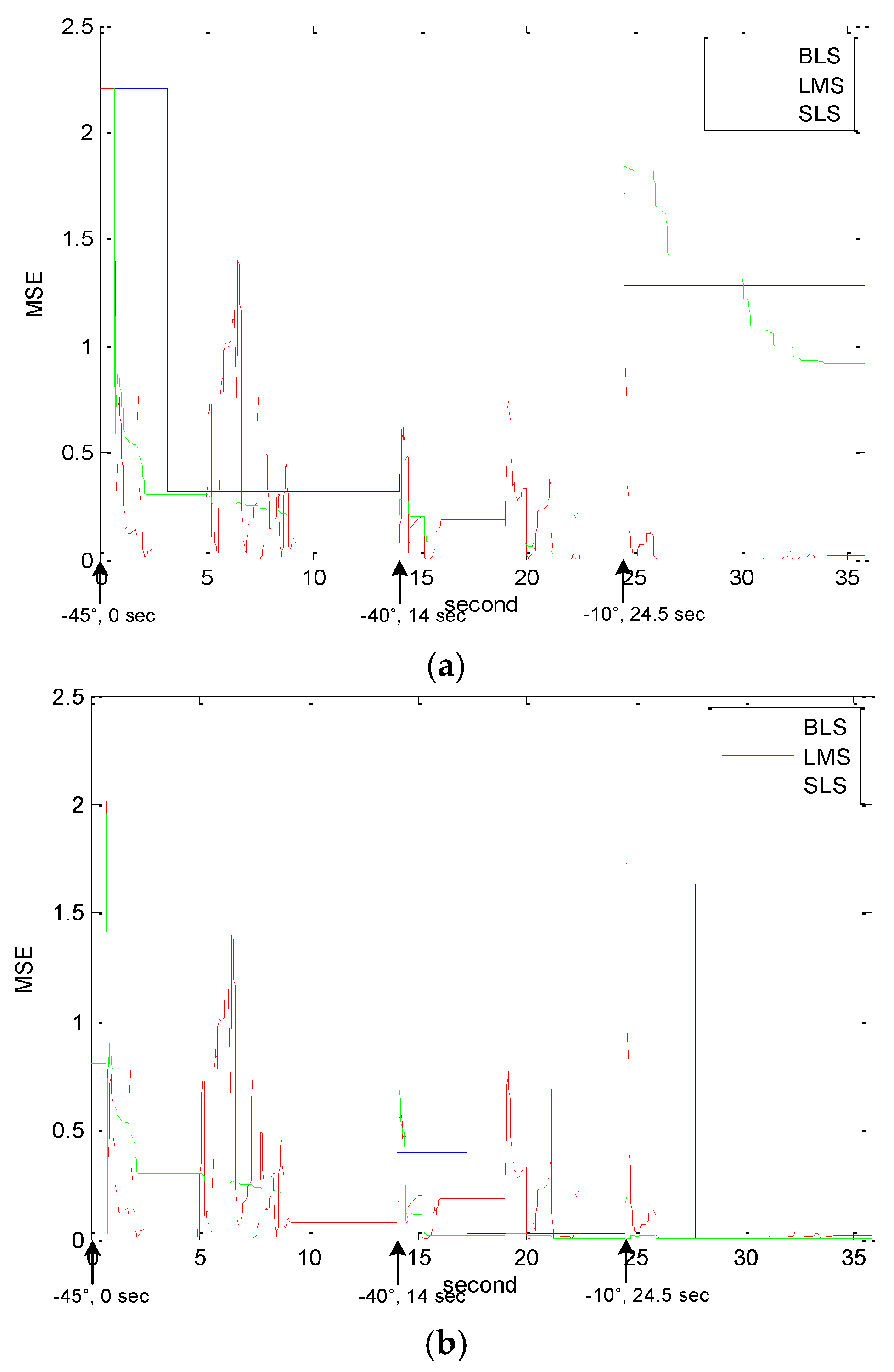
We conducted the evaluation to compare the two conventional methods—the BLS method [1,2] and LMS method [3]—with the proposed SLS method. Figure 3 and

Table 1. Averaged MSEs.

Methods	Averaged MSE
	“No Reset” Case, Averaged from 0 through 24.5 s in Figure 3a	“Reset” Case, Averaged during Entire Evaluation Period in Figure 3b
BLS	0.5978	0.4817
LMS	0.2360	0.1723
SLS	0.2052	0.1372

summarize the MSEs evaluated for the three methods. The “no reset” in Figure 3a and Table 1 means that the RTF estimate values of the BLS and the SLS methods were not reinitialized after the movement of the target. The proposed method shows a lower MSE than that of the BLS method on average because of its cumulative nature in the RTF estimation yielding more accurate values in the long run. The same cumulative nature, however, caused it to have greater errors at least in the earlier time frame when the speaker was at −10° (at 24.5 s). The adaptive nature of the SLS-based estimator corrected its RTF values to more accurate values than the one computed by the batch method after about five seconds. The errors exhibited by the SLS after 24.5 s are of an artificial nature in that the speaker location changed abruptly from −40° to −10°. In actual applications of beamforming in isolating the subject speaker from others, it is safe to assume that the subject speaker moves from one location to another at moderate speed. Therefore, it is very unlikely that a human speaker would move instantaneously from one location to another by 30° as it was the case in the experiment. The cumulative and gradual nature of updating the RTF in the case of the SLS approach is therefore more suitable for tracking and isolating a moving speaker.

In comparison to the LMS method, it is shown in Figure 3a that the performance of the proposed method declined when the sound source moved abruptly in large angles. Since our sequential method does not include any speech detector which would prompt re-initialization of the RTF estimates for any movement of the source, the data corresponding to previous positions of the source give rise to adverse effects on estimating the RTF when the source moves in large angles. Due to the speech detector coupled with the RTF estimation based on recursive updating, the LMS method shows reasonable performance after the sound source moved abruptly. The LMS method, however, was shown to be sensitive to noise as its performance degraded significantly between 5 and 9 s, and between 19 and 21 s intervals. Incorporating the speech detector in the processing may have led to incorrect RTF estimate values as the detector reacted to false alarms in these time intervals.

In another comparison of the three methods as depicted in Figure 3b, RTFs were re-initialized for both the batch method and the sequential method when the target source moved. Since the LMS method per se has the function of adapting to any environmental change [3], the initialization was unnecessary. In this evaluation, the proposed method shows the best performance in Table 1. The batch method needs an input data block in its initialization to estimate the RTF, therefore high MSE values appear in the duration corresponding to the beginning input data blocks: 0–3.2 s, 14.5–17.7 s and 25–28.2 s For the BLS to be capable to estimate the RTF, at least a 3.2 s block was required. In the experiments, it is not considered that the user moves within the BLS block size to see the performance of the algorithm itself (not due to insufficient data). Regardless of the block size and algorithms, the RTF value should be re-initialized with the corresponding data. Otherwise, it will show the simulation result as depicted in Figure 3a. That experiment simulated the situation:

• The targeted user started to speak initially at −45° and paused.
• 5° change) The user moved to −40 degrees and spoke again at 14 s and paused.
• (30° change) The user moved again to 10° and spoke again at 24.5 s.
• Figure 3a has shown that if the RFT is not initialized, the estimation error gets a higher value as the angular distance gets farther. When comparing the 5° (−45° to −40°) and 30° changes (−40° to −10°), it can be easily seen that the MSE gap increased significantly when the 30° change was made.

In the two experiments conducted, the proposed SLS method with re-initializations of the RTFs demonstrated the best performance among the considered methods in the case of a moving sound source. This result is promising considering that the angular position change of a sound source of interest occurs frequently in real-life environments, and such position change can be detected by another sensor as assumed in [9]. However, it must be reminded that the proposed method performed well when the source location change was moderate such as the 5° displacement as considered in the experiment. For following acoustic speech from a moving source, the SLS without any source position change detection may yet perform well in the current implementation.

5. Conclusions

We have presented a sequential approach to estimate the RTF for beamforming. The SLS method recursively updates the RTF estimates with the current input signal. Thus, it requires a minimal initialization period in the data collection and results in a significant reduction in the memory requirement. In addition to these advantages over the conventional estimation methods, it is shown that the proposed SLS improves the accuracies of the estimated RTF. Thus, we conclude that the proposed method is efficient and effective in estimating the RTF, and it has been shown in limited experimental trials that it exhibits notable improvements over existing methods.