Enhanced Video Classification System Using a Block-Based Motion Vector

Abstract

The main objective of this work was to design and implement a support vector machine-based classification system to classify video data into predefined classes. Video data has to be structured and indexed for any video classification methodology. Video structure analysis involves shot boundary detection and keyframe extraction. Shot boundary detection is performed using a two-pass block-based adaptive threshold method. The seek spread strategy is used for keyframe extraction. In most of the video classification methods, selection of features is important. The selected features contribute to the efficiency of the classification system. It is very hard to find out which combination of features is most effective. Feature selection makes relevance to the proposed system. Herein, a support vector machine-based classifier was considered for the classification of video clips. The performance of the proposed system considered six categories of video clips: cartoons, commercials, cricket, football, tennis, and news. When shot level features and keyframe features, along with motion vectors, were used, 86% correct classification was achieved, which was comparable with the existing methods. The research concentrated on feature extraction where combination of selected features was given to a classifier to get the best classification performance.

1. Introduction

Research on content-based visual information retrieval started in the 1990s. Earlier retrieval systems concentrated on image data based on visual content, such as color, texture, and shape [1]. In the early days, video retrieval systems only extended to image retrieval systems that segmented videos into shots and extracted keyframes from these shots. On the other hand, analyzing video content, which fully considers video temporality, has been an active research area for the past several years and is likely to attract even more attention in years to come [1]. Video data can be used for commercial, educational, and entertainment purposes. Due to the decreasing cost of storage devices, higher transmission rates, and improved compression techniques, digital video is available in an ever-increasing rate. All of these popularized the use of video data for retrieval, browsing, and searching. Due to its vast volume, effective classification techniques are required for efficient retrieval, browsing, and searching of video data.

Video data conveys particular visual information. Due to its content richness, video outperforms any other multimedia presentation. Content-based retrieval systems process information contained in a video’s data and creates an abstraction of its content in terms of visual attributes. Any query operation deals with this abstraction rather than the entire data, hence the term ‘content-based’. Similar to the text-based retrieval system, a content-based image or video retrieval system has to interpret the contents of a document’s collection (i.e., images or video records) and rank them according to the level of their relevance to the query.

Considering the large volume, video data needs to be structured and indexed for efficient retrieval. Content-based image retrieval technologies can be extended to video retrieval as well. However, such extension is not straightforward. A video clip or a shot is a sequence of image frames. Therefore, indexing each frame as still images involves high redundancy and increased complexity. Before indexing can be done, we need to identify the structure of the video and decompose it into basic components. Then, indices can be built based on structural information and information from individual image frames. In order to achieve this, the video data has to be segmented into meaningful temporal units or segments called video shots. A shot consists of a sequence of frames recorded continuously and representing a continuous action in time and space. The video data is then represented as a set of feature attributes such as color, texture, shape, motion, and spatial layout.

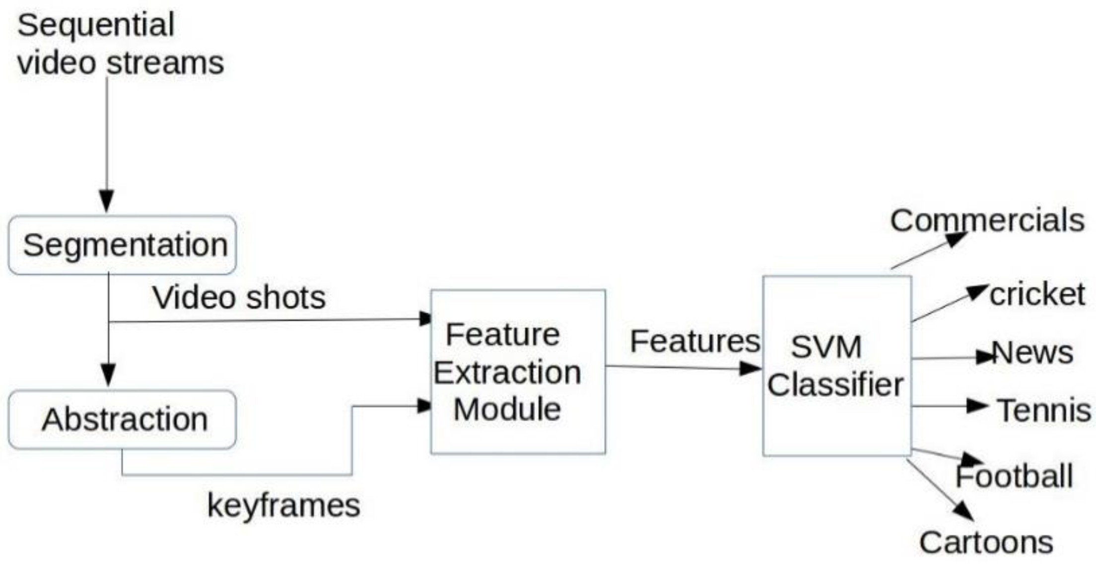
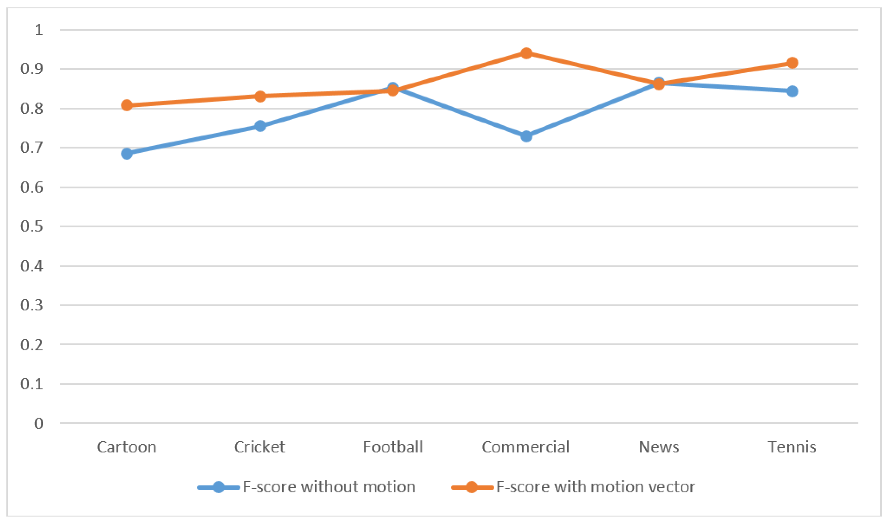
In this paper, we proposed an approach where spatio-temporal information was included with low-level features. During feature extraction, a group of frame descriptors was used to capture temporal information regarding video data and an edge histogram descriptor was used to obtain spatial information. Similarly, we associated a motion vector as a feature for capturing temporal information for efficient classification. All of these features were provided as inputs to the classifier.

The rest of the paper is organized as follows. Section 2 presents the summary of the related works. Section 3 contains methodology that includes segmentation, abstraction, feature extraction, and classification. Experimental results and comparison with state-of-the-art approaches are provided in Section 4. Result s and analysis are given in Section 5 and our concluding remarks are provided in Section 6.

2. Related Works

In recent years, automatic content-based video classification has emerged as an important problem in the field of video analysis and multimedia database. To access the query-based video database, approaches typically require users to provide an example video clip or sketch and the system should give the similar clips. The search for similar clips can be made efficient if the video data is classified into different genres. To help the users find and retrieve clips that are more relevant to the query, techniques need to be developed to categorize the data into one of the predefined classes. Ferman and Tekalp [2] employed a probabilistic framework to construct descriptors in terms of location, objects, and events. In our strategy, hidden Markov models (HMMs) and Bayesian belief networks (BBNs) were used at various stages to characterize content domains and extract relevant semantic information. A decision tree video indexing technique was considered in [3] to classify videos in genres such as music, commercials, and sports. A combination of several classifiers can improve the performance of individual classifiers, as was the case in [4].

Convolutional neural networks (CNNs) are used [5] for large scale video classification. In such instances, the run time performance improves via CNN architecture, which process inputs at two spatial resolutions. In [6], recurrent convolutional neural networks (RCNNs) were used for video classification tasks, which are good at learning relations from input sequences.

In [7], the authors investigated low-level audio–visual features for video classification. The features included Mel-frequency cepstrum coefficients (MFCC) and MPEG-7 visual descriptors such as scalable color, color layout, and homogeneous structure. 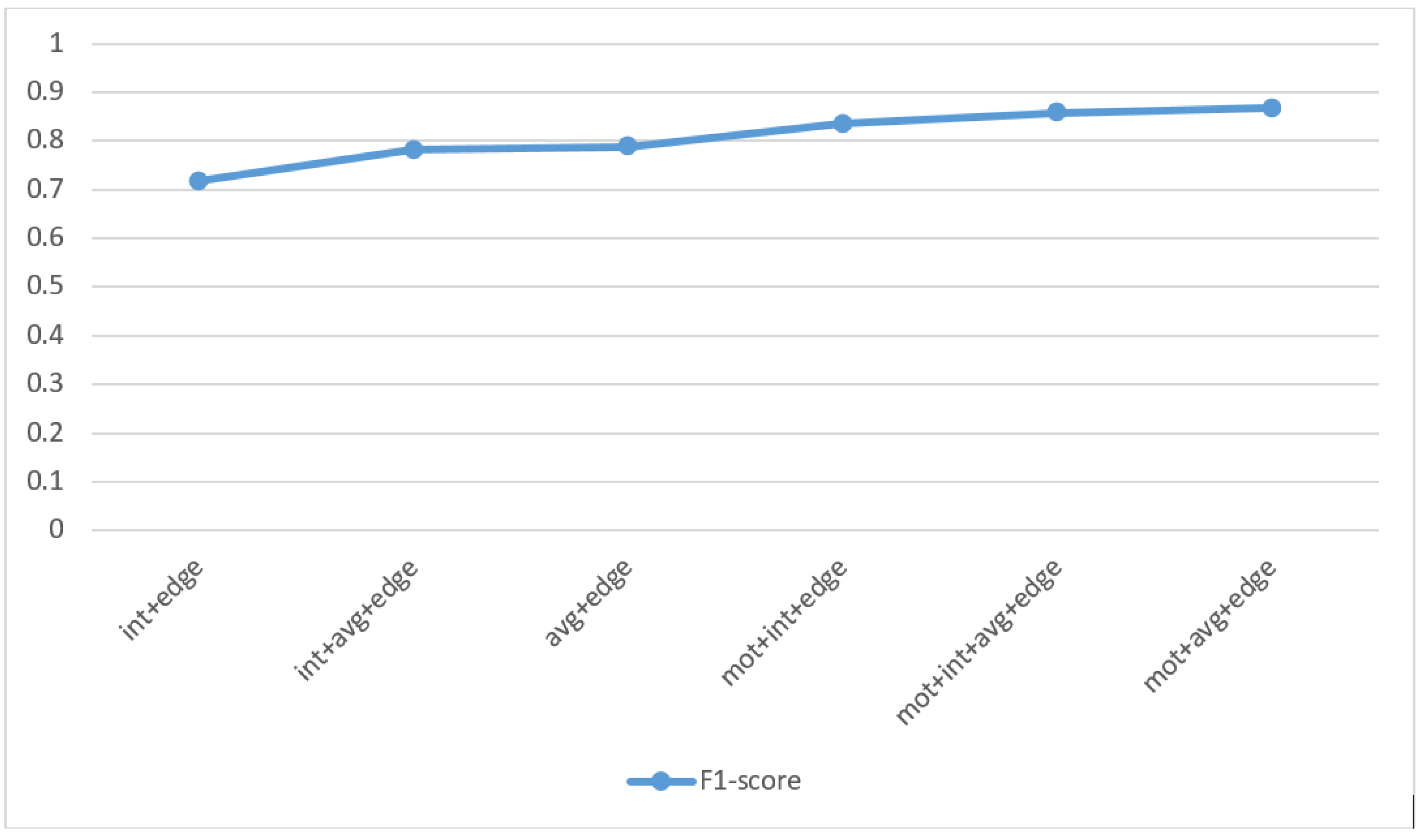Visual descriptors such as histogram-oriented gradients (HOG), histogram of optical flow (HOF), and motion boundary histograms (MBH) were used for video classification in [8]. Computational efficiency was achieved here for video classification using the bag-of-words pipeline. We placed more importance on computational efficiency than computational accuracy. In the proposed method, video classification was done using feature combinations of an edge-histogram, average histogram, and motion vector. This novel approach provided better results than the state-of-the-art methods.

The large size of the video files was a problem for efficient search for data and speedy retrieval of the relevant information required by the user. Therefore, videos were segmented into sequences of frames that represented continuous action in time and space. These sequences of frames are called video shots. The shot boundary detection algorithm is based on a comparison of color histograms of adjacent frames to detect those frames where image changes are significant. A shot boundary is hypothesized as follows: the distance between histograms of the current frame and the previous frame is higher than an absolute threshold. Many different shot detection algorithms have been proposed in order to automatically detect shot boundaries. The simplest way to measure the spatial similarity between the two frames ‘f_m’ and ‘f_n’ is via template matching. Another method to detect shot boundary is the histogram-based technique. The most popular metric for abrupt change or cut detection is finding the difference between the histograms of two consecutive frames. 2-D correlation coefficient techniques for video shot segmentation [9] uses statistical measurements with the assistance of motion vectors and Discrete Cosine Transform (DCT) coefficients from the MPEG stream. Afterwards, the heuristic models of abrupt or transitional scene changes can be confirmed through these measurements.

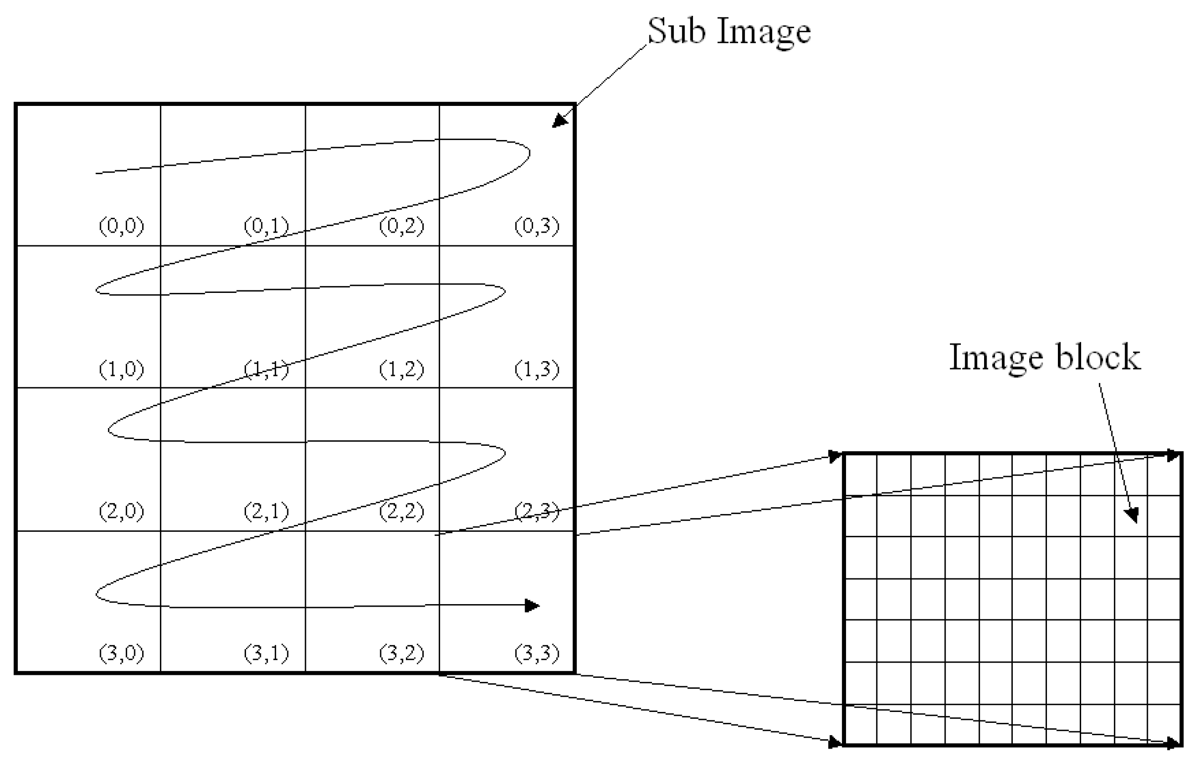
The twin-comparison algorithm [10] has been proposed to detect sharp cuts and gradual shot changes, which results in shot boundary detection based on a dual threshold approach. Another method used for shot boundary detection is the two-pass block-based adaptive threshold technique [11]. Five important parts of the frame with different priorities were used here for shot boundary detection. The adaptive threshold method was used for efficient detection. In our work, we used two pass block-based adaptive threshold methods for shot boundary detection.

Keyframes are frames that best represent a shot. One of the most commonly used keyframe extraction methods is based on a temporal variation of low-level color features and motion information proposed by Lin et.al. [12]. In this approach, frames in a shot are compared sequentially based on their histogram similarities. If a significant content change occurs, the current frame is selected as a keyframe. Such a process will be iterated until the last frame of the shot is reached. Another way of keyframe selection is through the clustering of video frames in a shot [13]. This employs a partitioned clustering algorithm with cluster-validity analysis to select the optimal number of clusters for shots. The frame closest to the cluster centroid is chosen as the keyframe. The seek-spread strategy is also based on the idea of searching for representative keyframes sequentially [14].

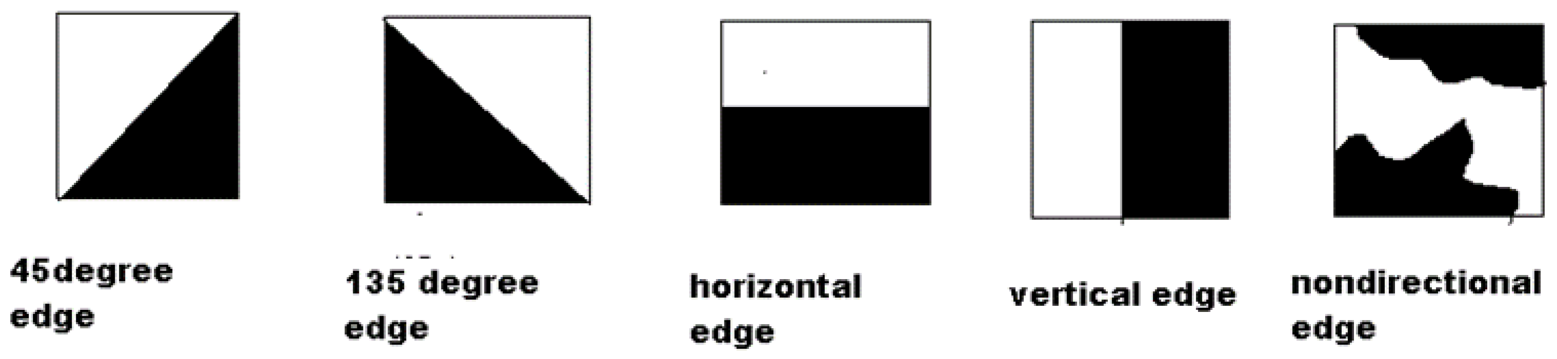
Feature extraction is the process of generating a set of descriptors or characteristic attributes from an image or video stream. Features taken into consideration can be broadly classified into frame level features and shot level features. Frame level features include color-based and texture-based features. Shot level features include the intersection histogram created from a group of frames. It also includes motion, defined as the temporal intensity change between successive frames, which is a unique character that distinguishes videos from other multimedia. By analyzing motion parameters, it is possible to distinguish between similar and different video shots or clips. In [9], for video object retrieval, motion estimation was performed with the help of Fourier Transform and L2 norm distance. The total motion matrix (TMM) [11] captures the total motion in terms of block-based measure by retaining the locality information of motion. It constructs 64-dimensional feature vector using the TMM, where each component represents the captured total spatial block motion of the entire frames in the video sequence. Motion features at pixel level is desirable to obtain motion information at a finer resolution. The pixel change ratio map (PCRM) [15] is used to index video segments as the basis of motion content. PCRM indicates moving regions in particular video sequence.

3. Methodology

The objective of this study was to design and implement an enhanced motion-based video classification system to classify video data into predefined classes. In the proposed approach, segmentation is done with the entire video stream by partitioning it into a sequence of logically independent segments called video shots. A shot consists of a sequence of frames. Video abstraction is the process of representing video shots with keyframes. Keyframes are extracted from shots. These frames best represent the content of a shot. The features are extracted from the shots as well as from keyframes represented as a feature vector. The support vector machines (SVMs) are trained using the selected features as the training data. In the testing phase, the SVMs classify the test data into a predefined class.

Figure 1 shows the schematic representation of the SVM-based classification of video content.

3.1. Segmentation

Video segmentation is the process of separating video data into meaningful parts called video shots, which are basic units that represent continuous action in time and space. After segmentation, we obtained video shots. In order to find shots, shot boundary had to be detected. Shot boundary detection is a process of detecting the boundaries between two consecutive shots so that a sequence of frames belonging to a single shot will be grouped together.

Shot Boundary Detection

In the proposed system, the two-pass block-based adaptive threshold technique was used [11] for shot boundary detection.

There are two passes in the algorithm. In the first pass, each frame was segmented at five corners namely top left (TL), top right (TR), middle (MID), bottom right (BT), and bottom left (BL) with units of size 60 × 60 pixels. Then, a quantized 64-bit RGB color histogram was created for each block. The accumulated histogram-based dissimilarity $S\left(f_m,f_n\right)$ between the two consecutive frames was determined as follows:

$$S(f_m,f_n)={\displaystyle \sum _{i=1}^r{B}_i\ast S_p(f_m,f_n,i)}$$

(1)

where B_i is the predetermined weighting factor. Partial match $S_p(f_m,f_n,i)$ was obtained using the histogram matching method. Here, f_m and f_n are consecutive frames and ‘r’ is the number of blocks. For all consecutive frames, the similarity difference is computed.

In the second pass, the sequence of dissimilarity measures computed in the first pass was chosen. A single adaptive threshold based on the Dugad model [16] was selected to detect the shot boundary. The dissimilarity measures from the previous and next few frames were used to adaptively set the shot boundary detection threshold. Thus, the method used a sliding window of a predetermined size where the samples within this window were considered. In practice, the mean and standard deviation of either side of the middle sample in the window were estimated. Then, the threshold was set as a function based on these statistics, as given below in Equation (2).

As per the Dugad model [16], the middle sample, $m_{\tau }$, represents a shot boundary if the following conditions below are simultaneously satisfied:

• The middle sample is the maximum in the window.
• The middle sample satisfies the condition as given in Equation (2).

$$m_{\tau }>max\left\{\left({\mu }_{left}+3\sqrt{{\sigma }_{left}}\right),\left({\mu }_{right}+3\sqrt{{\sigma }_{right}}\right)\right\}$$

(2)

where $m_{\tau }$ is the dissimilarity value of the two consecutive frames. ${\mu }_{left}$ represents the mean of the left samples of the middle sample and ${\mu }_{right}$ represents the mean of the right sample.

${\sigma }_{right}$ and ${\sigma }_{left}$ are the corresponding standard deviations.

3.2. Abstraction

Video abstraction is a process of extracting representative visual information about video, such as keyframes. By abstraction, we avoided processing a large number of video frames in a video shot, which also had redundancy. The result of the abstraction process formed a minimal number of frames from each video shot.

Keyframe Extraction

In this proposed system, the seek–spread strategy was used for keyframe extraction. The seek–spread strategy was also based on the idea of searching for representative keyframes sequentially [14]. This strategy has two stages. In the first stage, it compares the first frame to the following one until seeking a significantly different frame or reaching the end of the video shot. That new frame is selected as a keyframe. In the second stage, the strategy tries to spread over the representative range of that keyframe as far as possible. Again, the newly extracted keyframe is compared to the subsequent frames sequentially to select one more representative frame, if any, or until it reaches the end of the video shot.

The seek–spread strategy started and ended the frame of each video shot, and then it selected keyframes. Within a shot, the possible range of significant keyframes was selected as an extensive representative for the video shot content. To perform the frame similarity measure, a distance metric—as given in Equation (3) based on 64-color quantized global RGB color histogram and 60-bin quantized global HSV (hue-saturation value space)—color histogram was applied and normalized between 0.0 to 1.0 range. w₁ and w₂ were the predefined weight values ranging between 0.0 to 1.0 for both distance metrics, $D_{ch}\left(f_m,f_n\right)$ and $D_{hsv}\left(f_m,f_n\right)$ respectively.

$$S\left(f_m,f_n\right)=w_1\times D_{ch}\left(f_m,f_n\right)+w_2\times D_{hsv}\left(f_m,f_n\right)$$

(3)

$$\mathrm{where} D_{ch}\left(f_m,f_n\right)=\frac{{{\displaystyle \sum }}_{i=1}^N\left|H\left(f_m,i\right)-H\left(f_n,i\right)\right|}{{{\displaystyle \sum }}_{i=1}^{N}H\left(f_m,i\right)+{{\displaystyle \sum }}_{i=1}^{N}H\left(f_n,i\right)}$$

(4)

$$\mathrm{and} D_{hsv}\left(f_m,f_n\right)=w_j\times {{\displaystyle \sum }}_{j=1}^3\frac{{{\displaystyle \sum }}_{i=1}^N\left|H\left(f_m,i,j\right)-H\left(f_n,i,j\right)\right|}{{{\displaystyle \sum }}_{i=1}^{N}H\left(f_m,i,j\right)+{{\displaystyle \sum }}_{i=1}^{N}H\left(f_n,i,j\right)}$$

(5)

where i indicates the bin number and n indicates total number of bins.$D_{ch}\left(f_m,f_n\right)$ is the normalized RGB color quantized histogram-based distance metric for frames $f_m$ and $f_n$. Similarly, $D_{hsv}\left(f_m,f_n\right)$ is the HSV color quantized histogram-based distance metric for frames $f_m$ and $f_n$. j indicates the hue, saturation, and value components of the HSV color histogram, whereas $w_j$ indicates their corresponding predefined weight values.

3.3. Feature Extraction

Feature extraction is the process of generating a set of descriptors or characteristic attributes from an image or video stream. The performance of any classification system depends on the features used for video content representation. A two-level feature extraction, namely the frame level and shot level, was used in the proposed system.

3.3.1. Frame Level Feature Extraction

Frame level feature extraction is the process of extracting feature from an image or a frame. The descriptors or features can be broadly classified into global and local. Global feature extraction techniques transform the whole image into a functional representation where minute details in the individual portion of the multimedia can be ignored. On the other hand, local descriptors exhibit a fine-grained approach when analyzing data into segmented smaller regions. Local descriptors provide more effective characterization of a class. All these facts are taken into consideration when features are selected for classification. The features like color histogram and edge histogram descriptor are extracted from a frame.

Color Histogram

A color histogram is a histogram representation of an image by counting the ‘color’ of each pixel. The widely used image retrieval technique uses color histograms. In the histogram technique, the RGB color space is divided into “n” number of bins. For each image, a histogram is built by counting the number of pixels falling into each bin. During retrieval, the images are retrieved and ranked according to the histogram distances between the query image and images in databases. The most common distances used are the Manhattan and Euclidean distance.

Edge Histogram Descriptor

The edge histogram descriptor is a descriptor that describes the spatial distribution of four directional and non-directional edges in a still image. This descriptor expresses the local edge distribution in the image. In order to localize the edge distribution to a certain area of the image, the image is partitioned into 16 non-overlapping sub-images. Then, for each sub-image, an edge histogram to represent the edge distribution in the sub-image is generated. To characterize the sub-image, the edge distribution’s histogram for each sub-image is created. Edges in the sub-images are categorized into vertical, horizontal, 45-degree diagonal, 135-degree diagonal, and non-directed edges. The histogram for each sub-image represents the relative frequency of occurrence of the five types of edges in the corresponding sub-image. As a result, each local histogram contains 5 bins. Since there are 16 sub-images, 16 × 5 = 80 histogram bins are required.

In order to get the edge distribution of the sub-image, the sub-image is again divided into small square blocks called image-blocks. In each image block, the presence of five types of edges is found using the edge extraction method [17]. The image partition gives 16 equal sized sub-images, regardless of the size of the image. Next, 16 sub-images are visited in a raster scan order and the corresponding local bins are arranged accordingly. Figure 2 [17] depicts a sub-image and an image-block in an image. Figure 3 [17] shows the five types of edges taken into consideration.

To extract the directional edges features, we defined a small square block of 8 × 8 size image-blocks in each sub-image. A simple method to extract an edge feature in an image-block is to apply a digital filter in spatial domain. The sub-blocks were labelled from 0 to 3. The average gray levels of the pixels for four sub blocks in the (i,j)th image block were calculated and represented as a₀(i,j), a₁(i,j), a₂(i,j) and a₃(i,j), respectively. We represented the filter coefficients for vertical, horizontal, 45-degree diagonal, 135-degree diagonal, and non-directional edges as f_v(k), f_h(k), f_d-45(k), f_d-135(k), and f_nd(k), respectively [17].

The respective edge magnitudes m_v(i,j) m_h(i,j) m_d-45(i,j), m_d-135(i,j), and m_nd(i,j) for the (i,j)th image block were obtained as follows:

$$m_v\left(i,j\right)=\left|{\displaystyle \sum }_{k=0}^3{a}_k\left(i,j\right)f_v\left(k\right)\right|$$

(6)

$$m_h\left(i,j\right)=\left|{\displaystyle \sum }_{k=0}^3{a}_k\left(i,j\right)f_h\left(k\right)\right|$$

(7)

$$m_{d-45}\left(i,j\right)=\left|{\displaystyle \sum }_{k=0}^3{a}_k\left(i,j\right)f_{d-45}\left(k\right)\right|$$

(8)

$$m_{d-135}\left(i,j\right)=\left|{\displaystyle \sum }_{k=0}^3{a}_k\left(i,j\right)f_{d-135}\left(k\right)\right|$$

(9)

$$m_{nd}\left(i,j\right)=\left|{\displaystyle \sum }_{k=0}^3{a}_k\left(i,j\right)f_{nd}\left(k\right)\right|$$

(10)

If the maximum value among the 5 edge magnitudes obtained from Equations (6)–(10) was greater than the threshold value, then the image-block was considered to have the corresponding edge in it. Otherwise, the image block contained no edge. Based on the experiments conducted by Chee Sun Won et al. [17], the threshold value was taken as 11 since it gave better results when tested empirically. In the set of filter coefficients, the non-directed edge filter coefficient value taken was determined heuristically. In fact, the non-directional edges by definition did not have any directionality. Therefore, it was difficult to find filter coefficients that were applicable to all types of non-directional edges. To avoid this problem, the image block was classified into a monotone block and four directional edge blocks. The monotone block was a block that does not have edges. If the image-block did not belong to monotone or four directional edge blocks, then it was considered as a non-directional block.

We calculated the total number of five types of edges present in all image-blocks in the corresponding sub-image. Thus, for each sub-image, 5 bin values were obtained. Each image was divided into 16 non-overlapping sub-images and an 80-dimensional feature vector was obtained from each of it.

3.3.2. Shot Level Features

In the current literature, video shots are mostly represented by keyframes. Low-level features such as color, texture, and shape are extracted directly from the keyframes for indexing and retrieval. For efficiency, video retrieval is usually tackled in a similar way as image retrieval. Such a strategy, however, is ineffective since spatio-temporal information existing in videos is not fully exploited. In this proposed system, shot level features were used. Shot level features include the intersection histogram, average histogram [18], and motion vector, all of which were created from a group of frames to incorporate spatio-temporal information existing in videos.

Group of frames descriptors

The group of frames histogram descriptors are descriptors defined for a group of frames. For the retrieval of information from a video database, keyframes that best represent the shots are selected. Features of the entire collection of frames are represented within those keyframes. Such methods are highly dependent on the quality of the representative samples. Thus, a set of histogram-based descriptors that capture the color content of video frames can be used. A single representation for an entire collection can be obtained by combining the individual frame histograms in various ways. The three sub-descriptors used are the average histogram, median histogram, and intersection histogram [18]. In the proposed system, the intersection histogram and average histogram descriptors were created.

The intersection histogram provided the least common color traits of the given group of frames rather than the color distribution. The distinct property of the intersection histogram made it appropriate for fast identification of the group of frames in the query clip. The intersection histogram was generated by computing for each bin ‘j’, the minimum value over all frame histograms in the video shot.

$$\mathrm{int}-\mathrm{histogram}[j]=\underset{i}{\min }\left(Histogramvalu{e}_i\left[j\right]\right), j=1,\dots .,64$$

(11)

where Histogramvalue_i[j] is the jth bin of frame i of color histogram.

The average histogram is a histogram with an average value for each bin of all histograms in the group. Generally, it is computed by accumulating the individual frame histograms.

$$\mathrm{avg}-\mathrm{histogram}[j]=\underset{i}{\mathrm{Avg}}\left(Histogramvalu{e}_i\left[j\right]\right), j=1,\dots .,64$$

(12)

where Histogramvalue_i[j] is the jth bin of frame i of color histogram.

Average Block-Based Pixel Change Ratio Map

The human visual system perceives motion if the intensity of motion is high. In this study, the pixel change ratio map (PCRM) showed the intensity of motion in a video sequence. Changes in pixel intensity over all frames in the video shot were taken for classification. Intensity of motion depended on the object movement. The high intensity of motion resulted in a large change in pixel intensity over the frames. Motion, defined as the temporal intensity change between successive frames, is a unique character of video media when compared with others, such as audio or image. By analyzing these motion parameters, it was possible to distinguish between similar and different video shots.

To create PCRM [15], the size of the PCRM matrix had to be the same as the size M × N if the frames size was M × N. Initially, the PCRM matrix components were initialized to zero. For the current frame i, we added the absolute values of the frame differences p_i − p_I−1 and p_i+1 − p_i, i.e.,

$$D{I}_i=\left|p_i-p_{i-1}\right|+\left|p_{i+1}-p_i\right|$$

(13)

where $D{I}_i$ represents the sum of the absolute values of the frame differences p_i − p_I−1 and p_i+1 − p_i, p_i refers to pixel intensity value for each pixel p for the current frame i, $p_{i-1}$ refers to pixel intensity value for corresponding pixel p for the previous frame, and $p_{i+1}$ refers to pixel intensity value for each pixel p for the next frame. For each pixel in this frame, if the sum DI_i was greater than a threshold, the corresponding location in the PCRM was incremented by 1. This procedure was carried out for all frames in the video shot. The PCRM values were then divided by the number of frames and normalized to lie in [0, 1] for uniformity. Thus, it represented the ratio of the number of pixels whose intensities changed as a result of significant motion.

The proposed method used a novel average block-based PCRM. To get the average block-based PCRM, the PCRM for each shot was divided into 16 blocks. Then, the mean of each block was taken and a 16-dimensional feature vector was created. PCRM simply by itself does not include much information if it is used as such. By dividing into 16 blocks and taking the mean of it, however, it can reflect spatial information depending on the value. If the value is higher than it means more movement is there at that part of the video shot.

3.4. SVM Classification

Support vector machines are a popular technique for data classification. SVMs were proposed by Vapnik et al. as an effective method for a general-purpose supervised pattern recognition [19]. In the extraction module, features are extracted from shots and keyframes.

SVM is trained using these features as training data. In the testing phase, SVM classifies test data into predefined classes. SVM has the ability to generalize to unseen data. The performance of the pattern classification problem depends on the type of kernel function chosen. In this work, a Gaussian kernel was used.

4. Results

SVMs were originally designed for two-class classification problems. In our work, multi-class (M = 6) classification tasks were achieved using a one-against-the-rest approach, where an SVM was constructed for each class by discriminating that class against the remaining (M−1) classes. The features used were the intersection histogram, average histogram, edge histogram descriptor, and shot level motion vector. The different combinations of features were experimented with. The intersection histogram had 64 dimensions, the average histogram had 64 dimensions, the edge histogram had 80 dimensions, and the motion vector had 16 dimensions, all of which were used in different combinations. Out of 4292 examples, two-thirds of the data was used for training and one-third for testing.

The experiments were carried out on 600 video clips, each for 20 s captured at 25 frames per second. Video dataset included 6 categories: cartoons, commercials, cricket, football, tennis, and news. The data was collected from different TV channels on different dates and at different times to ensure a variety of data.

Subsequent subsections have showed results of different combinations of feature vectors with and without the motion vector. It is evident from the results the that motion vector played an important role in the efficient video classification system.

4.1. Combination of Features without the Motion Vector

In this case, we used different combinations of the edge histogram, intersection histogram, and average histogram to find the importance of including the proposed motion vector. Significant changes occurred when the motion vector was also used along with other features. Both of the cases were part of the experiment.

4.1.1. Combination of the Intersection Histogram and Edge Histogram

Initially, we combined the intersection histogram and edge histogram. We achieved 72% correct classification on the test data using these features.

Table 1. Confusion matrix for the video classification using the intersection histogram and edge histogram.

Cartoons	Cricket	Football	Commercials	News	Tennis
64.98	3.39	0.56	20.90	3.39	6.78
10.26	63.25	10.82	8.55	0.85	6.27
3.57	10	80.72	5.71	0	0
9.87	4.66	0.74	78.77	2.61	3.35
12.82	2.56	0	8.97	70.53	5.12
8.77	4.68	0	16.37	0.58	69.6

shows the SVM-based video classification performance when the intersection histogram and edge histogram were used as feature vectors.

From Table 1 it can be observed that, in the cartoon category, a misclassification is mainly with commercials and vice versa. This is a result of the similarity of the color characteristics of these two categories.

4.1.2. Combination of the Average Histogram and Edge Histogram

Instead of the previous combination, when the average histogram and edge histogram was used, an average of 78.14% correct classification was achieved. In this case, misclassification was mainly between the cartoon and commercial categories.

Table 2. Confusion matrix for the video classification using the average histogram and edge histogram.

Cartoons	Cricket	Football	Commercials	News	Tennis
67.14	3.29	0.47	24.88	3.28	0.94
5.90	80.08	6.64	5.17	0	2.21
2.33	13.37	78.49	5.81	0	0
11.03	3.23	0.38	81.56	1.9	1.9
3.95	9.21	0	3.95	80.26	2.63
5.61	3.06	0	12.24	0.51	78.6

shows the SVM-based video classification performance when the average histogram and the edge histogram were used as feature vectors.

4.1.3. Combination of the Intersection Histogram, Average Histogram, and Edge Histogram

When the test was conducted again using the combination of the feature vectors, average histogram, intersection histogram, and edge histogram, the same 78% correct classification was achieved.

Table 3. Confusion matrix for the video classification using the average histogram and edge histogram and intersection histogram.

Cartoons	Cricket	Football	Commercials	News	Tennis
64.13	1.79	0.45	22.87	7.62	3.14
7.12	81.14	6.05	2.14	0	3.55
2.35	13.53	79.41	3.53	0	1.18
10.09	2.52	0.37	81.98	2.52	2.52
3.23	9.68	0	1.61	77.42	8.06
5.52	1.22	0.61	8.59	0	84.1

shows the SVM-based video classification performance when the average histogram and the edge histogram were used as feature vectors.

4.2. Combination of Features with Motion Vector

It was observed that the motion vector had a very good classification impact when it was included with other features. Therefore, the average block-based pixel change ratio map was used with the intersection histogram and edge histogram. thus making it a 160 dimensional feature vector.

Table 4. Confusion matrix for the video classification using the motion vector, intersection histogram, and edge histogram.

Cartoons	Cricket	Football	Commercials	News	Tennis
86.63	8.11	5.5	0	0	0
7.31	90.43	1.68	0	0.2	0.3
6.55	6.9	80	3.6	0	2.9
1.9	0	7.1	89.61	0	1.3
20.51	5.1	0	0	74.35	0
4.52	6.78	9.03	1.12	0	78.53

shows the performance of this combination.

4.2.1. Combination of the Intersection Histogram, Edge Histogram, Motion Vector

Table 4 shows the confusion matrix for the video classification using the motion vector, intersection histogram, and edge histogram.

From the data given in the table we can observe that an average of 83% correct classification was achieved in this case.

4.2.2. Combination of the Average Histogram, Edge Histogram, and Motion Vector

Table 5. Confusion matrix for the video classification using the motion vector, average histogram, and edge histogram.

Cartoons	Cricket	Football	Commercials	News	Tennis
83.76	11.11	0.003	0	0	0
5.44	93.43	0.003	0	0	0.75
5.09	4.36	84	5.45	0	1.1
1.29	0	3.89	94.15	0	0.6
8.97	12.82	0	0	75.64	1.28
2..82	3.38	5.65	0.56	0	87.57

shows another combination of the motion vector, average histogram, and edge histogram which gives better results, i.e., an 86.42% correct classification.

4.2.3. Combination of the Average Histogram, Intersection Histogram, Edge Histogram, and Motion Vector

A combination of the average histogram, intersection histogram, edge histogram, and motion vector were used for the classification and confusion matrix. In this scenario, we achieved 86% correct classification. For classification, a 224 dimensional feature vector was given to SVM. This is indicated in

Table 6. Confusion matrix for the video classification using the motion vector, intersection histogram, average histogram, and edge histogram.

Cartoons	Cricket	Football	Commercials	News	Tennis
89.32	5.13	4.7	0	0	0.85
7.7	90	0.37	0.18	0	1.7
6.18	5.45	82.54	4.72	0	1.09
1.3	0	4.54	93.5	0	0.65
17.94	7.69	0	0	73.07	1.28
0.56	5.08	5.08	1.69	0	87.57

.

5. Result Analysis

The F-measure or F1 score is an evaluation metric most commonly used in classification problems. The F1 score provides equal weight when measuring precision and recall, and it is considered one of the best metrics to evaluate a classification model [20]. It considers both the precision p and recall r of a test to compute the F1 score. Here, p is the number of the correct positive results divided by the number of all positive results returned by the classifier, whereas r is the number of correct positive results divided by the number of all relevant samples (all samples that should have been identified as positive).

We can define precision and recall as follows:

$$P=\frac{\left|true positives\right|}{\left|true positives\right|+ \left|false positives\right|}$$

(14)

$$R=\frac{\left|true positives\right|}{\left|true positives\right|+\left|false negatives\right|}$$

(15)

The F1 score is the harmonic average of precision and recall, where an F1 score reaches its best value at 1 (perfect precision and recall) and worst at 0.

$${\mathrm{F}}_1=2\ast \frac{1}{\frac{1}{recall}+\frac{1}{precision}}=2\ast \frac{precision\ast recall}{precision+recall}$$

(16)

A good classification model should have good precision and high recall. The F-measure combines both of these aspects in a single metric. The F1 score is the weighted average of precision and recall. Therefore, this score takes both false positives and false negatives into account. Intuitively, it is not as easy to understand as accuracy, but the F1 score is usually more useful than accuracy, especially in an uneven class distribution. As the proposed method has an uneven class distribution, the F1 score is used.

The Figure 4 shows the F1 score for video classification.

The above graph reflects the importance of the motion vector when classifying videos into different categories. It can be seen that the F1 score obtained with an average histogram and edge histogram with and without using a motion vector had significant change. Cartoon, cricket, commercials, and tennis where motion intensity was high showed more precisely why they were classified.

From Figure 5, we inferred that the classification system obtained the best average F1 score when we used the feature combination of the average histogram, edge histogram, and motion vector. It shows that the feature combination of the average histogram, edge histogram, and motion vector gave the optimal performance for the classification model.

To measure the performance of the proposed model, we conducted a comparison against some of the existing classifiers. Every classifier used the feature combination of average histogram, edge histogram, and motion vector since it was more promising. SVM outperformed the other classifiers considered under comparison, such as the Naïve Bayes, K-nearest neighbor, and decision tree. This is indicated in

Table 7. Comparison of the proposed approach with different classifiers in terms of F1 scores and accuracy.

Classifiers	F1 Score	Accuracy Score
Naïve Bayes_BernoulliNB	0.727	0.757
Decision tree classifier	0.481	0.573
K-nearest neighbor classifier	0.764	0.779
SVM	0.86	0.864

.

6. Conclusions

The proposed work implemented a support vector machine-based video classification system. The video categories taken into consideration were cartoons, commercials, cricket, news, football, and tennis. Along with the low-level features, spatio-temporal information was also used for classification. The extracted features were used to model different categories. About 78% correct classification performance was achieved using the shot-based and keyframe features. About 86% correct classification was achieved when motion vectors also included as a shot-based feature along with other features. Classifiers were attributes to each class, which were a measurement value that reflected the degree of confidence that a specific input clip belonged to a given class. This information can be used to reduce the search space for a small number of categories.

The performance of the classification system can be improved by combining evidence from other modalities, such as audio and text. The use of semi-global and global edge histograms generated directly from the local edge histogram can increase the matching performance.