Article

Complex q-Rung Orthopair Fuzzy Aggregation Operators and Their Applications in Multi-Attribute Group Decision Making

1
School of Management Science and Engineering, Shandong University of Finance and Economics, Jinan 250015, China
2
Department of Mathematics & Statistics, International Islamic University Islamabad, Islamabad 44000, Pakistan
*
Authors to whom correspondence should be addressed.
Information 2020, 11(1), 5; https://doi.org/10.3390/info11010005
Submission received: 18 November 2019 / Revised: 16 December 2019 / Accepted: 16 December 2019 / Published: 20 December 2019
(This article belongs to the Special Issue Artificial Intelligence and Decision Support Systems)

Abstract

:
In this manuscript, the notions of q-rung orthopair fuzzy sets (q-ROFSs) and complex fuzzy sets (CFSs) are combined is to propose the complex q-rung orthopair fuzzy sets (Cq-ROFSs) and their fundamental laws. The Cq-ROFSs are an important way to express uncertain information, and they are superior to the complex intuitionistic fuzzy sets and the complex Pythagorean fuzzy sets. Their eminent characteristic is that the sum of the qth power of the real part (similarly for imaginary part) of complex-valued membership degree and the qth power of the real part (similarly for imaginary part) of complex-valued non-membership degree is equal to or less than 1, so the space of uncertain information they can describe is broader. Under these environments, we develop the score function, accuracy function and comparison method for two Cq-ROFNs. Based on Cq-ROFSs, some new aggregation operators are called complex q-rung orthopair fuzzy weighted averaging (Cq-ROFWA) and complex q-rung orthopair fuzzy weighted geometric (Cq-ROFWG) operators are investigated, and their properties are described. Further, based on proposed operators, we present a new method to deal with the multi-attribute group decision making (MAGDM) problems under the environment of fuzzy set theory. Finally, we use some practical examples to illustrate the validity and superiority of the proposed method by comparing with other existing methods.

1. Introduction

To dispose unknown or undetermined information in the field of decision making, Zadeh [1] proposed the innovative concept of fuzzy set (FS) in 1965, which is characterized by a membership function limited to [0, 1], and it has been proven to be a very powerful tool to deal with uncertain information in real-life problems. Now, there are many extensions of FSs, such as interval-valued fuzzy set was proposed by Zadeh [2]. Moreover, Coupland and John [3] pioneered the idea of geometric type-1 and type-2 fuzzy logic systems and applied in practical decision making problems. As mentioned above, although the fuzzy sets have many advantages, however there are some situations where it is difficult or impossible to solve the issue by using only membership function. To handle this issue, Atanassov [4] introduced the notion of intuitionistic fuzzy set (IFS) as a generalization of FS, which is characterized by membership function, non-membership function, and indeterminacy or inconsistency belonging to [0, 1]. The limitation of the IFS is that the sum of membership grade and non-membership grade is less than or equal to 1. The concept of IFS is a more powerful tool than FS to cope with uncertain problems, and it is also a better way to explain the opinion of human being. Further, this concept has drawn much attention and has been successfully applied in Mathematics, engineering, information sciences and multi-attribute decision making (MADM) problems [5,6,7,8,9]. Especially, for MADM problems, IFS has been an important technique to solve the different areas of decision making problems [10,11,12,13,14,15].
However, when a decision maker provides such type of values for membership grade and for non-membership grade, which cannot meet the condition that their sum must be in [0, 1] such as: 0 0.6 + 0.7 = 1.3 1 , obviously, this situation cannot be described by IFS. In order to overcome this shortcoming, Yager [16] proposed the notion of Pythagorean fuzzy set (PyFS), whose constraint is that the sum of square of membership degree and square of non-membership degree is less than or equal to 1. Furthermore, Zhang and Xu [17] proposed the TOPSIS methods to process the MCDM problems with the Pythagorean fuzzy information. Mete [18] extended the AHP-MOORA methods to process the MCDM problems with the Pythagorean fuzzy information. Yang et al. [19] extended the TOPSIS methods to process the MCDM problems with the Pythagorean fuzzy information. Garg [20] proposed some new generalized Pythagorean fuzzy information aggregations using Einstein operations and discussed their applications to decision making. Peng and Yang [21] proposed Pythagorean fuzzy Choquet integral and MABAC method based on Pythagorean fuzzy information. Grag [22] also presented the generalized Pythagorean fuzzy geometric aggregation operators using Einstein t-norm and t-conorm for Pythagorean fuzzy information. For more information related to PyFSs, we may refer to [23,24,25,26].
Although IFSs and the PyFSs can describe the uncertain information precisely, there are still problems that IFSs and PyFSs are unable to handle. For example, when a decision maker provides 0.7 for membership grade and 0.9 for non-membership grade, they have not satisfied the condition of PyFs such as 0.72 + 0.92 = 1.30 > 1. So, for this type of problem, Yager [27] introduced the notion of q-rung orthopair fuzzy set (q-ROFS) which is a more powerful and more general than IFS and PyFS to deal with complicated and uncertain information in the environment of fuzzy set theory. Further, Liu and Wang [28] introduced the q-ROF aggregation operators for averaging the evaluation information. The q-ROF Bonferroni mean operators for q-ROFS information was investigated by Liu and Liu [29]. Peng et al. [30] presented the exponential operations and aggregation operator for q-ROFS, and the other researches for the q-ROFS were also developed [31,32,33,34,35,36,37].
However, many researchers also asked a question, what will be happened when we change the co-domain of FS to some set of complex numbers instead of [0, 1]. The answer of this question was given by Ramot [38] in 2002, who defined the concept of complex fuzzy set (CFS) as a generalization of FS. The CFS is characterized by a complex valued function, i.e., M τ ( x ) = T τ ( x ) . e i . 2 π W T τ ( x ) and satisfied the condition: 0 T τ ( x ) , W T τ ( x ) 1 . The notion related to CFSs are also proposed in [39,40,41]. As mentioned above, although the complex fuzzy sets have many advantages, however there are some situations where it is difficult or impossible to solve the issue by using only complex-valued membership function. To handle this issue, Alkouri and Salleh [42] proposed the novelty of complex IFS (CIFS), where the CIFS is characterized by complex valued membership and complex valued non-membership. The constraint of the CIFS is that the sum of the real part (similarly for imaginary part) of complex-valued membership degree and the real part (similarly for imaginary part) of complex-valued non-membership degree is equal to or less than 1. To overcome the information of periodicity and uncertainty at the same time which is related to “complex” functionality. For further work related to CIFS and their drawbacks, we may refer to [43,44,45,46,47,48,49,50,51].
As we all know that CIFSs have the complex-valued membership and complex-valued non-membership functions, so it may be difficult to describe some complicated complex intuitionistic fuzzy information, for example, when a decision maker provides 0.7 e i 2 π ( 0.71 ) for membership grade and 0.6 e i 2 π ( 0.61 ) for non-membership grade, the CIFSs cannot describe this result i.e., 0.7 + 0.6 = 1.3 1 and 0.71 + 0.61 = 1.32 1 . For dealing such types of situations, Ullah et al. [52] introduced complex pythagorean fuzzy set (CPyFS), whose constraint is that the sum of the square of real part (similarly for imaginary part) of complex-valued membership grade and square of the real part (similarly for imaginary part) of complex-valued non-membership grade is less than or equal to one. The constraint of the CPYFS is more general than CIFS i.e., 0.7 2 + 0.6 2 = 0.49 + 0.36 = 0.85 1 and 0.71 2 + 0.61 2 = 0.50 + 0.37 = 0.87 1 . They have greater expressiveness than CIFSs, therefore, CFSs have also received much attention from researchers. For example, Akram and Naz [53] proposed the idea of complex pythagorean fuzzy graph.
CPyFS and CIFS theory have been widely used by the researchers, but due to the complexity of the decision making problems, sometimes decision-makers are not suitable to provide their judgment in form of single-valued membership and non-membership degrees. Consequently, an extension of the existing theories might be extremely valuable to depict the uncertainties because of his/her reluctant judgment in complex decision-making problems. Therefore, to provide the more freedom to the decision makers, it is advisable to ask the experts to describe their preferences by means of intervals.
Same situation occurs in CIFS and CPyFS, when the decision maker provides these types of data, which do not satisfy the conditions of CIFS and the condition of CPyFS. For example, a decision maker provides 0.9 e i 2 π ( 0.8 ) for complex-valued membership grade and 0.8 e i 2 π ( 0.7 ) for complex-valued non-membership grade, the CIFSs and CPyFSs cannot describe this result i.e., 0.9 + 0.8 = 1.7 1 ,   0.8 + 0.7 = 1.5 1 and 0.9 2 + 0.8 2 = 0.81 + 0.64 = 1.45 1 ,   0.8 2 + 0.7 2 = 0.64 + 0.49 = 1.13 1 . For dealing with such types of situations, in this article we examine the novel approach of complex q-rung orthopair fuzzy sets (Cq-ROFSs) and their fundamental operational laws. Their eminent characteristic is that the sum of the qth power of the real part (Similarly for imaginary part) of complex-valued membership degree and the qth power of the real part (Similarly for imaginary part) of complex-valued non-membership degree is equal to or less than 1, i.e., 0.9 5 + 0.8 5 = 0.92 1 ,   0.8 5 + 0.7 5 = 0.5 1 . The proposed Cq-ROFS is an important technique to deal with uncertain and more difficult information and then apply it to solve the multi-attribute decision making (MADM) problems. The Cq-ROFS is more generalized than existing methods like complex Pythagorean fuzzy set (CPyFS) and complex intuitionistic fuzzy set (CIFS). If we will take the imaginary part is zero, in the terms of membership grade and non-membership grade, then the proposed approach is convert into q-rung Orthopair fuzzy set (q-ROFS). q-ROFS is the special case of the proposed method. If we considered the value of parameter q = 1 in the environment of q-ROFS, then the q-ROFS is converted for intuitionistic fuzzy set (IFS). Similarly, if we considered the value of parameter q = 2 in the environment of q-ROFS, then the q-ROFS is converted for Pythagorean fuzzy set (PyFS). The IFS and PyFS are the particular cases of the proposed approaches. Therefore, the motivation and goal of this paper are shown as follows.
(1)
Propose the notion of Cq-ROFS and some operational laws, and then explain their characteristics and comparison method;
(2)
Develop some extended aggregation operators, such as complex q-rung orthopair fuzzy weighted averaging operator (Cq-ROFWAO), complex q-rung orthopair fuzzy weighted geometric operator (Cq-ROFWGO), and then verify their properties;
(3)
Develop a new MADM method based on the proposed operators;
(4)
Give some examples to show the flexibility and superiority of the developed method.
The construct of this manuscript is followed as: In Section 2, we review some basic notions of PyFSs, CPyFSs, q-ROFSs, and their properties, while in Section 3, we proposed Cq-ROFSs by extending each value of the membership and non-membership functions from real number to complex number of the unit circle. We also proposed some basic operations on Cq-ROFS. In Section 4, we introduced the aggregation operators such as averaging and geometric operators. In Section 5, we used the example to show the steps of the MADM problems. further, we described the advantages of our proposed work and also gave the comparative study. The conclusion of this paper is discussed in last section.

2. Preliminaries

In this Section, we give the basic definitions of PyFSs, CPyFSs, q-ROFSs, and their properties. For convenience, in this paper, we use X is to represent the non-empty finite discourse set, and M τ ( x ) and N τ ( x ) to express the membership and non-membership grade in X and T τ ( x ) , F τ ( x ) , W T τ ( x ) , W F τ ( x ) [ 0 ,   1 ] and i = 1 .
Definition 1.
[16] A PyFS τ is defined as: τ = { ( x , M τ ( x ) , N τ ( x ) ) / x X } where M τ : X [ 0 ,   1 ] , N τ : X [ 0 ,   1 ] satisfying the conditions: 0 M τ 2 ( x ) + N τ 2 ( x ) 1 . The term H τ ( x ) = ( 1 ( M τ 2 ( x ) + N τ 2 ( x ) ) ) 1 2 is considered as hesitancy degree of x . Further τ = ( M τ , N τ ) is called a Pythagorean fuzzy number (PyFN).
Definition 2.
[52] A CPyFS τ is defined as τ = { ( x , M τ ( x ) , N τ ( x ) ) / x X } where M τ : X { z 1 : z 1 τ ,   | z 1 | 1 } N τ : X { z 2 : z 2 τ ,   | z 2 | 1 } such that M τ ( x ) = z 1 = a 1 + i b 1 and N τ ( x ) = z 2 = a 2 + i b 2 provided that 0 | z 1 | 2 + | z 2 | 2 1 or M τ ( x ) = T τ ( x ) . e i . 2 π W T τ ( x ) and N τ ( x ) = F τ ( x ) . e i . 2 π W F τ ( x ) satisfying the conditions: 0 T τ 2 ( x ) + F τ 2 ( x ) 1 and 0 W T τ 2 ( x ) + W F τ 2 ( x ) 1 . Moreover, the term H τ ( x ) = R . e i . 2 π W R c ( x ) such that R = ( 1 ( T τ 2 ( x ) + F τ 2 ( x ) ) ) 1 2 and W R ( x ) = ( 1 ( W T τ 2 ( x ) + W F τ 2 ( x ) ) ) 1 2 is considered as Complex hesitancy degree of x . Further τ = ( T . e i . 2 π W T , F . e i . 2 π W F ) is called a complex pythagorean fuzzy number (CPyFN).
Definition 3.
[27] A q-ROFS τ is defined as: τ = { ( x , M τ ( x ) , N τ ( x ) ) / x X } where M τ : X [ 0 , 1 ] , N τ : X [ 0 ,   1 ] satisfying the conditions: 0 M τ q ( x ) + N τ q ( x ) 1   , ( q > 1 ) . The term is considered as hesitancy degree of x . Further τ = ( M τ , N τ ) is called a q-rung orthopair fuzzy number (q-ROFN).
Definition 4.
[27] Let τ j = ( M j , N j ) ,   j = 1 , 2 be any two q-ROFNs and let γ > 0 be any real number, then we have
(1) 
τ 1 τ 2 = ( ( M 1 q + M 2 q M 1 q M 2 q ) 1 q , ( N 1 N 2 ) ) ;
(2) 
τ 1 τ 2 = ( ( M 1 M 2 ) , ( N 1 q + N 2 q N 1 q N 2 q ) 1 q ) ;
(3) 
γ τ J = ( ( 1 ( 1 M j q ) γ ) 1 q , N j γ ) ,   j = 1 , 2 ;
(4) 
τ J γ = ( M j γ , ( 1 ( 1 N j q ) γ ) 1 q ) ,   j = 1 , 2 .

3. Complex q-Rang Orthopair Fuzzy Set

In this Section, we propose the novel approach of Cq-ROFS, also to propose some basic operations.
Definition 5.
A Cq-ROFS τ is defined as τ = { ( x , M τ ( x ) , N τ ( x ) ) / x X } where M τ : X { z 1 : z 1 τ ,   | z 1 | 1 } N τ : X { z 2 : z 2 τ ,   | z 2 | 1 } such that M τ ( x ) = z 1 = a 1 + i b 1 and N τ ( x ) = z 2 = a 2 + i b 2 provided that 0 | z 1 | q + | z 2 | q 1 or M τ ( x ) = T τ ( x ) . e i . 2 π W T τ ( x ) and N τ ( x ) = F τ ( x ) . e i . 2 π W F τ ( x ) satisfying the conditions: 0 T τ q ( x ) + F τ q ( x ) 1 and 0 W T τ q ( x ) + W F τ q ( x ) 1 . Moreover, the term H τ ( x ) = R . e i . 2 π W R c ( x ) such that R = ( 1 ( T τ q ( x ) + F τ q ( x ) ) ) 1 / q and W R ( x ) = ( 1 ( W T τ q ( x ) + W F τ q ( x ) ) ) 1 / q is considered as Complex hesitancy degree of x . Further τ = ( T . e i . 2 π W T , F . e i . 2 π W F ) is called a Cq-ROFN.
Where, M τ ( x ) and N τ ( x ) of Cq-ROFS are clearly complex numbers in polar/Cartesian form. Further we are taking T τ ( x ) = F τ ( x ) = r and 2 π .   W T τ ( x ) = θ 1 ,   2 π . W F τ ( x ) = θ 2 then these two types of notations are interconvertible as follows:
M τ ( x ) = T τ ( x ) . e i . 2 π W T τ ( x ) = T τ ( x ) .   ( τ o s   2 π W T τ ( x ) + i S i n   2 π W T τ ( x ) )     = T τ ( x ) . τ o s   2 π W T τ ( x ) + i T τ ( x ) . S i n   2 π W T τ ( x )     = r . τ o s   θ 1 + i r . S i n   θ 1 = a 1 + i b 1 = z 1 ,
N τ ( x ) = F τ ( x ) . e i . 2 π W F τ ( x ) = F τ ( x ) .   ( τ o s   2 π W F τ ( x ) + i S i n   2 π W F τ ( x ) )     = F τ ( x ) . τ o s   2 π W F τ ( x ) + i F τ ( x ) . S i n   2 π W F τ ( x ) = r . τ o s   θ 2 + i r . S i n   θ 2     = a 2 + i b 2 = z 2 .
Here we will demonstrate the limitation of CIFS and show the advantages of Cq-ROFS by some examples.
Consider an example of CIFS of the form { ( x ,   ( 0.499 +   0.016   i ) ,   ( 0.298 +   0.036   i ) ) } . This set satisfies the basic definition of CIFS as | 0.499 +   0.016   i | = 0.499 and | 0.498 + 0.036   i | = 0.499 and 0 0.499 + 0.298 1 . The polar form of this CIFNs is { ( x ,   0.499   e i   ( 0.016 ) ,   0.298   e i   ( 0.036 ) ) } .
On the other hand, consider the representation of an uncertain event as { ( x ,   0.799948 + 0.029363 i ,   0.496693 + 0.06267   i ) } . Then | 0.799948 + 0.029363 i | = 0.8 and | 0.496693 + 0.06267   i | = 0.5 and 0 0.8 + 0.5 1 . This means that CIFS is not enough to deal with this type of information. However, the concept of Cq-ROFS can handle such information 0 0.7 2 + 0.6 2 = 0.85 1 . Hence, the number, { ( x ,   0.799948 + 0.029363 i ,   0.496693 + 0.06267   i ) } which can be written as { ( x ,   0.799948   e i   ( 0.029363 ) ,   0.496693   e i   ( 0.06267 ) ) } , is considered as a Cq-ROFN.
The following Figure 1 shows the comparison of the restrictions of CIFS and CFS.
Similar to the operations of CIFSs and CFSs, now we will propose the basic operations like inclusion, complement, and equality of Cq-ROFSs.
Remark 1.
Every CIFS can be considered as Cq-ROFS but not conversely.
Definition 6.
For a two Cq-ROFNs A = { T A ( x ) . e i . 2 π W T A ( x ) , F A ( x ) . e i . 2 π W F A ( x ) } and B = { T B ( x ) . e i . 2 π W T B ( x ) , F B ( x ) . e i . 2 π W F B ( x ) } , then
(1) 
A B iff T A ( x ) T B ( x ) ,   F A ( x ) F B ( x ) and W T A ( x ) W T B ( x ) ,   W F A ( x ) W F B ( x ) .
(2) 
A = B iff T A ( x ) = T B ( x ) ,   F A ( x ) = F B ( x ) and W T A ( x ) = W T B ( x ) ,   W F A ( x ) = W F B ( x ) .
(3) 
A c = { F A ( x ) . e i . 2 π W F A ( x ) , T A ( x ) . e i . 2 π W T A ( x ) } .
Definition 7.
A score function S and accuracy function H on τ = ( T . e i . 2 π W T , F . e i . 2 π W F ) is defined as:
S ( τ ) = 1 2 | ( T q F q ) + ( W T q W F q ) | ,
H ( τ ) = 1 2 | ( T q + F q ) + ( W T q + W F q ) | .
where ( τ ) [ 1 ,   1 ] , H ( τ ) [ 0 ,   1 ] .
Definition 8.
An order relation between two Cq-ROFNs τ and τ ˙ is can be defined as
1. 
If S ( τ ) > S ( τ ˙ ) then τ > τ ˙ ,
2. 
If S ( τ ) = S ( τ ˙ ) and
(1) 
If H ( τ ) > H ( τ ˙ ) then τ > τ ˙ .
(2) 
If H ( τ ) = H ( τ ˙ ) then τ = τ ˙ .
Remark 2. (Monotonicity of score function).
Let τ = ( T . e i . 2 π W T , F . e i . 2 π W F ) be a Cq-ROFN. Then, the score function S ( τ ) = 1 2 | ( T q F q ) + ( W T q W F q ) | , is a monotonic increasing function with T ,   W T , and a monotonic decreasing function with F , W F .
Theorem 1. (Symmetry of score function).
Let τ j = ( T j . e i . 2 π W T j , F j . e i . 2 π W F j ) ,   j = 1 , 2 be two Cq-ROFNs, then τ j c = ( F j . e i . 2 π W F j , T j . e i . 2 π W T j ) ,   j = 1 , 2 is their associated inverse (complement) function respectively. Then we have the following conclusion S ( τ 1 ) S ( τ 2 ) if and only if S ( τ 2 c ) S ( τ 1 c ) .
Proof. 
By Definition 9, applying on Cq-RFNs τ j = ( T j . e i . 2 π W T j , F j . e i . 2 π W F j ) ,   j = 1 , 2 , we have
S ( τ 1 ) = 1 2 | ( T 1 q F 1 q ) + ( W T 1 q W F 1 q ) | ,
S ( τ 2 ) = 1 2 | ( T 2 q F 2 q ) + ( W T 2 q W F 2 q ) | .
By direct part we assume that
  • S ( τ 1 ) S ( τ 2 ) if and only if | ( T 1 q F 1 q ) + ( W T 1 q W F 1 q ) | | ( T 2 q F 2 q ) + ( W T 2 q W F 2 q ) |
  • S ( τ 1 ) S ( τ 2 ) if and only if | ( F 1 q + T 1 q ) + ( W F 1 q + W T 1 q ) | | ( F 2 q + T 2 q ) + ( W F 2 q + W T 2 q ) |
  • S ( τ 1 ) S ( τ 2 ) if and only if S ( τ 2 c ) S ( τ 1 c ) .
 □
Remark 3. (Monotonicity of accuracy function).
Let τ = ( T . e i . 2 π W T , F . e i . 2 π W F ) be a Cq-ROFN, then the accuracy function H ( τ ) = 1 2 | ( T q + F q ) + ( W T q + W F q ) | is a monotonic increasing function with T ,   W T , F , W F .
Remark 4. (Symmetry of accuracy function).
Let τ j = ( T j . e i . 2 π W T j , F j . e i . 2 π W F j ) ,   j = 1 , 2 be two Cq-ROFNs, then τ j c = ( F j . e i . 2 π W F j , T j . e i . 2 π W T j ) ,   j = 1 , 2 is their associated inverse (complement) function respectively. Then we have H ( τ 1 ) = H ( τ 2 ) .
Next, we will propose the operational laws for Cq-ROFNs based on the Archimedean t-norm operations as follows.
Definition 9.
Let τ j = ( T j . e i . 2 π W T j , F j . e i . 2 π W F j ) ,   j = 1 , 2 be any two Cq-ROFNs and let γ > 0 be any real number, then we have
τ j c = ( F j . e i . 2 π W F j , T j . e i . 2 π W T j ) ,   j = 1 , 2 ;
τ 1 τ 2 = ( m a x ( T 1 , T 2 ) . e i . 2 π . m a x ( W T 1 , W T 2 ) , m i n ( F 1 , F 2 ) . e i . 2 π . m i n ( W F 1 , W F 2 ) ) ;
τ 1 τ 2 = ( m i n ( T 1 , T 2 ) . e i . 2 π . m i n ( W T 1 , W T 2 ) , m a x ( F 1 , F 2 ) . e i . 2 π . m a x ( W F 1 , W F 2 ) ) ;
τ 1 τ 2 = ( ( T 1 q + T 2 q T 1 q T 2 q ) 1 q . e i . 2 π . ( W T 1 q + W T 2 q W T 1 q W T 2 q ) 1 q , ( F 1 F 2 ) . e i . 2 π ( W F 1 W F 2 ) ) ;
τ 1 τ 2 = ( ( T 1 T 2 ) . e i . 2 π ( W T 1 W T 2 ) , ( F 1 q + F 2 q F 1 q F 2 q ) 1 q . e i . 2 π . ( W F 1 q + W F 2 q W F 1 q W F 2 q ) 1 q ) ;
γ τ J = ( ( 1 ( 1 T j q ) γ ) 1 q . e i . 2 π ( 1 ( 1 W T j q ) γ ) 1 q , F j γ . e i . 2 π W F j γ ) ,   j = 1 , 2 ;
τ J γ = ( T j γ . e i . 2 π W T j γ , ( 1 ( 1 F j q ) γ ) 1 q . e i . 2 π ( 1 ( 1 W F j q ) γ ) 1 q ) ,   j = 1 , 2 .
Theorem 2.
Let τ j = ( T j . e i . 2 π W T j , F j . e i . 2 π W F j ) ,   j = 1 , 2 be any two Cq-ROFNs and let n 1 , n 2 > 0 be any real number, then we have
τ 1 τ 2 = τ 2 τ 1 ;
τ 1 τ 2 = τ 2 τ 1 ;
n 1 ( τ 1 τ 2 ) = n 1 τ 1 n 1 τ 2 ;
n 1 τ 1 n 2 τ 1 = ( n 1 + n 2 ) τ 1 ;
τ 1 n 1 τ 1 n 2 = τ 1 n 1 + n 2 ;
τ 1 n 1 τ 2 n 1 = ( τ 1 τ 2 ) n 1 .
Proof. 
We are investigating Equations (10), (12), and (14) and the others are straightforward.
  • For Equation (10), we have
    τ 1 τ 2 = ( ( T 1 q + T 2 q T 1 q T 2 q ) 1 q . e i . 2 π . ( W T 1 q + W T 2 q W T 1 q W T 2 q ) 1 q , ( F 1 F 2 ) . e i . 2 π ( W F 1 W F 2 ) ) = ( ( T 2 q + T 1 q T 2 q T 1 q ) 1 q . e i . 2 π . ( W T 2 q + W T 1 q W T 2 q W T 1 q ) 1 q , ( F 2 F 1 ) . e i . 2 π ( W F 2 W F 1 ) ) = τ 2 τ 1
  • Obviously.
  • For Equation (12), for the left hand, we have
    n 1 ( τ 1 τ 2 ) = n 1 ( ( T 1 q + T 2 q T 1 q T 2 q ) 1 q . e i . 2 π . ( W T 1 q + W T 2 q W T 1 q W T 2 q ) 1 q , ( F 1 F 2 ) . e i . 2 π ( W F 1 W F 2 ) ) = ( ( ( 1 ( 1 ( T 1 q + T 2 q T 1 q T 2 q ) ) n 1 ) 1 q ) q . e i . 2 π . ( ( 1 ( 1 ( W T 1 q + W T 2 q W T 1 q W T 2 q ) ) n 1   ) 1 q ) q , ( F 1 F 2 ) n 1 . e i . 2 π ( W F 1 W F 2 ) n 1 )
    For right hand, we have
    n 1 τ 1 = ( ( 1 ( 1 T 1 q ) n 1 ) 1 q . e i . 2 π ( 1 ( 1 W T 1 q ) n 1 ) 1 q , F 1 n 1 . e i . 2 π W F 1 n 1 )
    and
    n 1 τ 2 = ( ( 1 ( 1 T 2 q ) n 1 ) 1 q . e i . 2 π ( 1 ( 1 W T 2 q ) n 1 ) 1 q , F 2 n 1 . e i . 2 π W F 2 n 1 )
    then, we have
    n 1 τ 1 n 1 τ 2 = ( ( 1 ( 1 T 1 q ) n 1 ) 1 q . e i . 2 π ( 1 ( 1 W T 1 q ) n 1 ) 1 q , F 1 n 1 . e i . 2 π W F 1 n 1 ) ( ( 1 ( 1 T 2 q ) n 1 ) 1 q . e i . 2 π ( 1 ( 1 W T 2 q ) n 1 ) 1 q , F 2 n 1 . e i . 2 π W F 2 n 1 ) = ( ( ( ( 1 ( 1 T 1 q ) n 1 ) 1 q ) q + ( ( 1 ( 1 T 2 q ) n 1 ) 1 q ) q ( ( 1 ( 1 T 1 q ) n 1 ) 1 q ) q ( ( 1 ( 1 T 2 q ) n 1 ) 1 q ) q ) 1 q . e i . 2 π ( ( ( 1 ( 1 W T 1 q ) n 1 ) 1 q ) q + ( ( 1 ( 1 W T 2 q ) n 1 ) 1 q ) q ( ( 1 ( 1 W T 1 q ) n 1 ) 1 q ) q ( ( 1 ( 1 W T 2 q ) n 1 ) 1 q ) q ) 1 q ( F 1 F 2 ) n 1 . e i . 2 π ( W F 1 W F 2 ) n 1 , ) = ( ( 1 ( 1 T 1 q T 2 q + T 1 q T 2 q ) n 1 ) 1 q . e i . 2 π . ( 1 ( 1 W T 1 q W T 2 q + W T 1 q W T 2 q ) n 1 ) 1 q , ( F 1 F 2 ) n 1 . e i . 2 π ( W F 1 W F 2 ) n 1 ) = ( ( 1 ( 1 ( T 1 q + T 2 q T 1 q T 2 q ) ) n 1 ) 1 q . e i . 2 π . ( 1 ( 1 ( W T 1 q + W T 2 q W T 1 q W T 2 q ) ) n 1   ) 1 q , ( F 1 F 2 ) n 1 . e i . 2 π ( W F 1 W F 2 ) n 1 )
    Hence Equation (12) has provided.
  • Obviously.
  • For the Equation (14), we have
    τ 1 n 1 = ( T 1 n 1 . e i . 2 π W T 1 n 1 , ( 1 ( 1 F 1 q ) n 1 ) 1 q . e i . 2 π ( 1 ( 1 W F 1 q ) n 1 ) 1 q )
    and
    τ 1 n 2 = ( T 1 n 2 . e i . 2 π W T 1 n 2 , ( 1 ( 1 F 1 q ) n 2 ) 1 q . e i . 2 π ( 1 ( 1 W F 1 q ) n 2 ) 1 q ) .
    then, we have
    τ 1 n 1 τ 1 n 2 = ( T 1 n 1 . e i . 2 π W T 1 n 1 , ( 1 ( 1 F 1 q ) n 1 ) 1 q . e i . 2 π ( 1 ( 1 W F 1 q ) n 1 ) 1 q ) ( T 1 n 2 . e i . 2 π W T 1 n 2 , ( 1 ( 1 F 1 q ) n 2 ) 1 q . e i . 2 π ( 1 ( 1 W F 1 q ) n 2 ) 1 q ) = ( ( T 1 n 1 T 1 n 2 ) . e i . 2 π ( W T 1 n 1 W T 1 n 2 ) , ( ( ( 1 ( 1 F 1 q ) n 1 ) 1 q ) q + ( ( 1 ( 1 F 1 q ) n 2 ) 1 q ) q ( ( 1 ( 1 F 1 q ) n 1 ) 1 q ) q ( ( 1 ( 1 F 1 q ) n 2 ) 1 q ) q ) 1 q . e i . 2 π ( ( ( 1 ( 1 W F 1 q ) n 1 ) 1 q ) q + ( ( 1 ( 1 W F 1 q ) n 2 ) 1 q ) q ( ( 1 ( 1 W F 1 q ) n 1 ) 1 q ) q ( ( 1 ( 1 W F 1 q ) n 2 ) 1 q ) q ) 1 q ) = ( ( T 1 n 1 T 1 n 2 ) . e i . 2 π ( W T 1 n 1 W T 1 n 2 ) , ( 1 ( 1 F 1 q ) n 1 ( 1 F 1 q ) n 2 ) 1 q . e i . 2 π ( 1 ( 1 W F 1 q ) n 1 ( 1 W F 1 q ) n 2 ) 1 q ) = ( T 1 n 1 + n 2 . e i . 2 π W T 1 n 1 + n 2 , ( 1 ( 1 F 1 q ) n 1 + n 2 ) 1 q . e i . 2 π ( 1 ( 1 W F 1 q ) n 1 + n 2 ) 1 q ) = τ 1 n 1 + n 2
    Hence τ 1 n 1 τ 1 n 2 = τ 1 n 1 + n 2 .
  • Obviously.
 □

4. Some Complex q-Rung Orthopair Fuzzy Aggregation Operators

In this section, we propose some aggregation operators, which are the Cq-ROFWA operator and the Cq-ROFWG operator respectively. Where, ω = ( ω 1 , ω 2 , ω k ) T denoted the weight vectors and j = 1 k ω j = 1 , ω j [ 0 , 1 ] ,   j = 1 , 2 , , k . Moreover τ j = ( T j . e i . 2 π W T j , F j . e i . 2 π W F j ) ,   j = 1 , 2 , , k are represented the collection of Cq-ROFNs.
Definition 10.
The Cq-ROFWA is described as:
C q R O F W A : M k M ,   i f
C q R O F W A ( τ 1 , τ 2 , , τ k ) = ω 1 τ 1 ω 2 τ 2 ω k τ k = j = 1 k ω j τ j
Based on the operational laws of the Cq-ROFNs, we give the following Theorem.
Theorem 7.
Let us consider Definition 10, then we can obtain
C q R O F W A ( τ 1 , τ 2 , , τ k ) = ( ( ( 1 j = 1 k ( 1 T j q ) ω j ) 1 q . e i . 2 π ( 1 j = 1 k ( 1 W T j q ) ω j ) 1 q ) , j = 1 k F j ω j . e i . 2 π ( j = 1 k W F j ω j ) )
Proof. 
We used the mathematical indication to prove Equation (17), we have
Case 1. For k = 2 , since
ω 1 τ 1 = ( ( 1 ( 1 T 1 q ) ω 1 ) 1 q . e i . 2 π ( 1 ( 1 W T 1 q ) ω 1 ) 1 q , F 1 ω 1 . e i . 2 π W F 1 ω 1 ) ,
and
ω 2 τ 2 = ( ( 1 ( 1 T 2 q ) ω 2 ) 1 q . e i . 2 π ( 1 ( 1 W T 2 q ) ω 2 ) 1 q , F 2 ω 2 . e i . 2 π W F 2 ω 2 ) ,
then
C q R O F W A ( τ 1 , τ 2 ) = ω 1 τ 1 ω 2 τ 2 = ( ( 1 ( 1 T 1 q ) ω 1 ) 1 q . e i . 2 π ( 1 ( 1 W T 1 q ) ω 1 ) 1 q , F 1 ω 1 . e i . 2 π W F 1 ω 1 ) ( ( 1 ( 1 T 2 q ) ω 2 ) 1 q . e i . 2 π ( 1 ( 1 W T 2 q ) ω 2 ) 1 q , F 2 ω 2 . e i . 2 π W F 2 ω 2 ) = ( ( ( ( 1 ( 1 T 1 q ) ω 1 ) 1 q ) q + ( ( 1 ( 1 T 2 q ) ω 2 ) 1 q ) q ( ( 1 ( 1 T 1 q ) ω 1 ) 1 q ) q ( ( 1 ( 1 T 2 q ) ω 2 ) 1 q ) q ) 1 q . e i . 2 π ( ( ( 1 ( 1 W T 1 q ) ω 1 ) 1 q ) q + ( ( 1 ( 1 W T 2 q ) ω 2 ) 1 q ) q ( ( 1 ( 1 W T 1 q ) ω 1 ) 1 q ) q ( ( 1 ( 1 W T 2 q ) ω 2 ) 1 q ) q ) 1 q ( F 1 ω 1 F 2 ω 2 ) . e i . 2 π ( W F 1 ω 1 W F 2 ω 2 ) , ) = ( ( 1 ( 1 T 1 q ) ω 1 ( 1 T 2 q ) ω 2 ) 1 q . e i . 2 π ( 1 ( 1 W T 1 q ) ω 1 ( 1 W T 2 q ) ω 2 ) 1 q , ( F 1 ω 1 F 2 ω 2 ) . e i . 2 π ( W F 1 ω 1 W F 2 ω 2 ) ) = ( ( ( 1 j = 1 2 ( 1 T j q ) ω j ) 1 q . e i . 2 π ( 1 j = 1 2 ( 1 W T j q ) ω j ) 1 q ) , j = 1 2 F j ω j . e i . 2 π ( j = 1 2 W F j ω j ) )
Obviously, Equation (17) is kept.
Case 2. Let k = m , then Equation (17) holds.
C q R O F W A ( τ 1 , τ 2 , , τ m ) = ( ( ( 1 j = 1 m ( 1 T j q ) ω j ) 1 q . e i . 2 π ( 1 j = 1 m ( 1 W T j q ) ω j ) 1 q ) , j = 1 m F j ω j . e i . 2 π ( j = 1 m W F j ω j ) )
Case 3. We check for k = m + 1 , we have
C q R O F W A ( τ 1 , τ 2 , , τ m + 1 ) = ( ( ( 1 j = 1 m ( 1 T j q ) ω j ) 1 q . e i . 2 π ( 1 j = 1 m ( 1 W T j q ) ω j ) 1 q ) , j = 1 m F j ω j . e i . 2 π ( j = 1 m W F j ω j ) ) ω m + 1 τ m + 1 = ( ( ( ( ( 1 j = 1 m ( 1 T j q ) ω j ) 1 q ) q + ( ( 1 ( 1 T m + 1 q ) ω m + 1 ) 1 q ) q ( ( 1 j = 1 m ( 1 T j q ) ω j ) 1 q ) q ( ( 1 ( 1 T m + 1 q ) ω m + 1 ) 1 q ) q ) 1 q . e i .2 π ( ( ( 1 j = 1 m ( 1 W T j q ) ω j ) 1 q ) q + ( ( 1 ( 1 W T m + 1 q ) ω m + 1 ) 1 q ) q ( ( 1 j = 1 m ( 1 W T j q ) ω j ) 1 q ) q ( ( 1 ( 1 W T m + 1 q ) ω m + 1 ) 1 q ) q ) 1 q j = 1 m F j ω j F m + 1 ω m + 1 . e i . 2 π ( j = 1 m W F j ω j W F m + 1 ω m + 1 ) ) , ) = ( ( ( 1 j = 1 m + 1 ( 1 T j q ) ω j ) 1 q . e i . 2 π ( 1 j = 1 m + 1 ( 1 W T j q ) ω j ) 1 q ) , j = 1 m + 1 F j ω j . e i . 2 π ( j = 1 m + 1 W F j ω j ) )
So Equation (17) is kept. □
Remark 5.
From Theorem 3, we can prove that the result of C q R O F W A ( τ 1 , τ 2 , , τ k ) is still a Cq-ROFN.
(1) 
For the real part, we have
T = ( 1 j = 1 m + 1 ( 1 T j q ) ω j ) 1 q and F = j = 1 m + 1 F j ω j , and because 0 T j , F j 1 . Then, we have
0 1 T j q 1 0 ( 1 T j q ) ω j 1 0 j = 1 k ( 1 T j q ) ω j 1 0 ( 1 j = 1 m + 1 ( 1 T j q ) ω j ) 1 q 1 ; 0 F j ω j 1 0 j = 1 k F j ω j 1 .
So 0 T j , F j 1 .
T j q + F j q 1 , then F j q 1 T j q F j ω j ( 1 T j q ) ω j j = 1 k F j ω j j = 1 k ( 1 T j q ) ω j
0 T j q + F j q = ( ( 1 ( j = 1 k ( 1 T j q ) ω j ) ) 1 q ) q + ( j = 1 k F j ω j ) q = 1 j = 1 k ( 1 T j q ) ω j + ( j = 1 k F j ω j ) q 1 j = 1 k ( 1 T j q ) ω j + j = 1 k ( 1 T j q ) ω j = 1
So 0 T j q + F j q 1
(2) 
For the imaginary parts, it can also be proven clearly.
So, it is also a Cq-ROFN and Theorem 3 is proven.
Example 1.
Let τ 1 = ( 0.6 e i . 2 π ( 0.7 ) , 0.8 e i . 2 π ( 0.5 ) ) , τ 2 = ( 0.5 e i . 2 π ( 0.5 ) , 0.9 e i . 2 π ( 0.8 ) ) , τ 3 = ( 0.6 e i . 2 π ( 0.25 ) , 0.75 e i . 2 π ( 0.78 ) ) and τ 4 = ( 0.56 e i . 2 π ( 0.57 ) , 0.88 e i . 2 π ( 0.78 ) ) be four Cq-ROFNs and ω = ( 0.35 , 0.1 , 0.25 , 0.3 ) T be the weight vectors, then we determined the Cq-ROFWA operator for q = 4 such that
C q R O F W A ( τ 1 , τ 2 , τ 3 , τ 4 ) = ( ( ( 1 j = 1 4 ( 1 T j q ) ω j ) 1 q . e i . 2 π ( 1 j = 1 4 ( 1 W T j q ) ω j ) 1 q ) , j = 1 4 F j ω j . e i . 2 π ( j = 1 4 W F j ω j ) ) = ( ( 0.91 ) .56 e i . 2 π ( 0.89 ) , ( 0.55 ) e i . 2 π ( 0.58 ) ) .
Theorem 4. (Idempotent).
Let Cq-ROFNs τ j = τ = ( T . e i . 2 π W T , F . e i . 2 π W F ) , j = 1 , 2 , , k , then
Cq ROFWA ( τ 1 , τ 2 , τ 3 , , τ k ) = τ
Proof. 
Because
C q R O F W A ( τ 1 , τ 2 , τ 3 , , τ k ) = ( ( ( 1 j = 1 k ( 1 T j q ) ω j ) 1 q . e i . 2 π ( 1 j = 1 k ( 1 W T j q ) ω j ) 1 q ) , j = 1 k F j ω j . e i . 2 π ( j = 1 k W F j ω j ) ) = ( ( ( 1 j = 1 k ( 1 T q ) ω j ) 1 q . e i . 2 π ( 1 j = 1 k ( 1 W T q ) ω j ) 1 q ) , j = 1 k F ω j . e i . 2 π ( j = 1 k W F ω j ) ) = ( ( ( 1 ( 1 T q ) j = 1 k ω j ) 1 q . e i . 2 π ( 1 ( 1 W T q ) j = 1 k ω j ) 1 q ) , F j = 1 k ω j . e i . 2 π ( W F j = 1 k ω j ) ) = ( T . e i . 2 π W T , F . e i . 2 π W F ) = τ .
 □
Theorem 5. (Monotonicity).
Let the Cq-ROFNs τ j = ( T j . e i . 2 π W T j , F j . e i . 2 π W F j ) and τ j = ( T j . e i . 2 π W T j , F j . e i . 2 π W F j ) j = 1 , 2 , , k , if T j T j , F j F j , W T j W T j and W F j W F j , then
C q R O F W A ( τ 1 , τ 2 , τ 3 , , τ k ) C q R O F W A ( τ 1 , τ 2 , τ 3 , , τ k )
 □
Proof. 
Because T j T j , F j F j , W T j W T j and W F j W F j , then
1 T j q 1 T j q ( ( 1 ( j = 1 k ( 1 T j q ) ω j ) ) 1 q ) q ( ( 1 ( j = 1 k ( 1 T j q ) ω j ) ) 1 q ) q j = 1 k F j ω j j = 1 k F j ω j
and similarly for imaginary parts such that
1 W T j q 1 W T j q ( ( 1 ( j = 1 k ( 1 W T j q ) ω j ) ) 1 q ) q ( ( 1 ( j = 1 k ( 1 W T j q ) ω j ) ) 1 q ) q j = 1 k W F j ω j j = 1 k W F j ω j
Combing the both real and imaginary parts, we have
( ( ( 1 ( j = 1 k ( 1 T j q ) ω j ) ) 1 q ) q . e i . 2 π ( ( 1 ( j = 1 k ( 1 W T j q ) ω j ) ) 1 q ) q j = 1 k F j ω j . e i . 2 π j = 1 k W F j ω j ) ( ( ( 1 ( j = 1 k ( 1 T j q ) ω j ) ) 1 q ) q . e i . 2 π ( ( 1 ( j = 1 k ( 1 W T j q ) ω j ) ) 1 q ) q j = 1 k F j ω j . e i . 2 π j = 1 k W F j ω j )
We assume that C q R O F W A ( τ 1 , τ 2 , τ 3 , , τ k ) = τ and C q R O F W A ( τ 1 , τ 2 , τ 3 , , τ k ) = τ , so using the Equation (2), we have
S ( τ ) S ( τ ) .
Here there are two possibility which are discussed one by one.
  • When S ( τ ) > S ( τ ) , then by Definition 7, we have
    τ q R O F W A ( τ 1 , τ 2 , τ 3 , , τ k ) > τ q R O F W A ( τ 1 , τ 2 , τ 3 , , τ k ) ;
  • When S ( τ ) = S ( τ ) , then we have
    ( ( ( 1 ( j = 1 k ( 1 T j q ) ω j ) ) 1 q ) q . e i . 2 π ( ( 1 ( j = 1 k ( 1 W T j q ) ω j ) ) 1 q ) q j = 1 k F j ω j . e i . 2 π j = 1 k W F j ω j ) = ( ( ( 1 ( j = 1 k ( 1 T j q ) ω j ) ) 1 q ) q . e i . 2 π ( ( 1 ( j = 1 k ( 1 W T j q ) ω j ) ) 1 q ) q j = 1 k F j ω j . e i . 2 π j = 1 k W F j ω j )
Because T j T j , F j F j , W T j W T j and W F j W F j , then
( ( 1 ( j = 1 k ( 1 T j q ) ω j ) ) 1 q ) q = ( ( 1 ( j = 1 k ( 1 T j q ) ω j ) ) 1 q ) q j = 1 k F j ω j = j = 1 k F j ω j
and similarly for imaginary parts such that
( ( 1 ( j = 1 k ( 1 W T j q ) ω j ) ) 1 q ) q = ( ( 1 ( j = 1 k ( 1 W T j q ) ω j ) ) 1 q ) q j = 1 k W F j ω j = j = 1 k W F j ω j
Because the score functions are equal, then we used the accuracy function such that
H ( τ ) = ( ( ( 1 ( j = 1 k ( 1 T j q ) ω j ) ) 1 q ) q . e i . 2 π ( ( 1 ( j = 1 k ( 1 W T j q ) ω j ) ) 1 q ) q j = 1 k F j ω j . e i . 2 π j = 1 k W F j ω j ) = 1 2 ( ( ( 1 ( j = 1 k ( 1 T j q ) ω j ) ) 1 q ) q + j = 1 k F j ω j + ( ( 1 ( j = 1 k ( 1 W T j q ) ω j ) ) 1 q ) q + j = 1 k W F j ω j ) = 1 2 ( ( ( 1 ( j = 1 k ( 1 T j q ) ω j ) ) 1 q ) q + j = 1 k F j ω j   + ( ( 1 ( j = 1 k ( 1 W T j q ) ω j ) ) 1 q ) q + j = 1 k W F j ω j ) = ( ( ( 1 ( j = 1 k ( 1 T j q ) ω j ) ) 1 q ) q . e i . 2 π ( ( 1 ( j = 1 k ( 1 W T j q ) ω j ) ) 1 q ) q j = 1 k F j ω j . e i . 2 π j = 1 k W F j ω j ) = H ( τ ) .
From case (1) and (2), this Theorem is kept. □
Theorem 6. (Boundedness).
Let τ j = ( T j . e i . 2 π W T j , F j . e i . 2 π W F j ) , j = 1 , 2 , , k be the collection of Cq-ROFNs, if τ j + = ( m a x 1 j k T j . e i . 2 π m a x 1 j k W T j , m i n 1 j k F j . e i . 2 π m i n 1 j k W F j ) and τ j = ( m i n 1 j k T j · e i . 2 π m i n 1 j k W T j , m a x 1 j k F j · e i . 2 π m a x 1 j k W F j ) then
τ j C q R O F W A ( τ 1 , τ 2 , τ 3 , , τ k ) τ j +
Proof. 
We also discussed two case separately for membership and non-membership grades (for real and imaginary parts).
  • For membership grade of C q R O F W A ( τ 1 , τ 2 , τ 3 , , τ k ) , we get
    ( 1 ( j = 1 k ( 1 min 1 j k T j q ) ω j ) ) 1 q ( 1 ( j = 1 k ( 1 T j q ) ω j ) ) 1 q ( 1 ( j = 1 k ( 1 max 1 j k T j q ) ω j ) ) 1 q
    ( 1 ( ( 1 min 1 j k T j q ) j = 1 k ω j ) ) 1 q ( 1 ( j = 1 k ( 1 T j q ) ω j ) ) 1 q ( 1 ( ( 1 max 1 j k T j q ) j = 1 k ω j ) ) 1 q
    Because j = 1 k ω j = 1 , so
    min 1 j k T j ( 1 ( j = 1 k ( 1 T j q ) ω j ) ) 1 q max 1 j k T j
  • non-membership grade of C q R O F W A ( τ 1 , τ 2 , τ 3 , , τ k ) , we obtain
    j = 1 k min 1 j k F j ω j j = 1 k F j ω j j = 1 k max 1 j k F j ω j
    min 1 j k F j j = 1 k ω j j = 1 k F j ω j max 1 j k F j j = 1 k ω j
And because j = 1 k ω j = 1 so
min 1 j k F j j = 1 k F j ω j max 1 j k F j
Then combined the above two cases, we have
min 1 j k F j j = 1 k F j ω j max 1 j k F j
By the score function, we get
S ( τ ) S ( τ ) S ( τ + ) .
So according to the cases (1) and (2) and definition of score function, we obtain
τ j C q R O F W A ( τ 1 , τ 2 , τ 3 , , τ k ) τ j + .
 □
Next, we will discuss the special cases of our proposed operator.
  • If q = 1 , then Cq-ROFWA (Equation (17)) is reduced to CIFWA, i.e.,
    τ j C q R O F W A ( τ 1 , τ 2 , τ 3 , , τ k ) τ j + .
    C q R O F W A ( τ 1 , τ 2 , , τ k )      = ( ( ( 1 j = 1 k ( 1 T j 1 ) ω j ) 1 . e i . 2 π ( 1 j = 1 k ( 1 W T j 1 ) ω j ) 1 ) , j = 1 k F j ω j . e i . 2 π ( j = 1 k W F j ω j ) ) = C I F W A ( τ 1 , τ 2 , , τ k )
  • If q = 2 , then Cq-ROFWA (Equation (17)) is reduced to PyIFWA, i.e.,
    C q R O F W A ( τ 1 , τ 2 , , τ k )      = ( ( ( 1 j = 1 k ( 1 T j 2 ) ω j ) 1 2 . e i . 2 π ( 1 j = 1 k ( 1 W T j 2 ) ω j ) 1 2 ) , j = 1 k F j ω j . e i . 2 π ( j = 1 k W F j ω j ) ) = C P y F W A ( τ 1 , τ 2 , , τ k )
Next, we will propose the notion of Cq-ROFWG operator.
Definition 11.
The Cq-ROFWG is described as:
C q R O F W G : M k M ,   i f
C q R O F W G ( τ 1 , τ 2 , , τ k ) = τ 1 ω 1 τ 2 ω 2 τ k ω k = j = 1 k τ j ω j
Base on the operational laws of the Cq-ROFNs, we can obtain the following Theorem.
Theorem 7.
Let us consider the Definition (11), then we obtain
C q R O F W G ( τ 1 , τ 2 , , τ k )      = ( j = 1 k T j ω j . e i . 2 π ( j = 1 k W T j ω j ) , ( ( 1 j = 1 k ( 1 F j q ) ω j ) 1 q . e i . 2 π ( 1 j = 1 k ( 1 W F j q ) ω j ) 1 q ) )
Proof. 
Straightforward. (Similar to Theorem 3). □
Example 2.
Let τ 1 = ( 0.6 e i . 2 π ( 0.7 ) , 0.8 e i . 2 π ( 0.5 ) ) , τ 2 = ( 0.5 e i . 2 π ( 0.5 ) , 0.9 e i . 2 π ( 0.8 ) ) , τ 3 = ( 0.6 e i . 2 π ( 0.25 ) , 0.75 e i . 2 π ( 0.78 ) ) and τ 4 = ( 0.56 e i . 2 π ( 0.57 ) , 0.88 e i . 2 π ( 0.78 ) ) be four Cq-ROFNs and ω = ( 0.35 , 0.1 , 0.25 , 0.3 ) T be the weight vector. Then we calculate the Cq-ROFWA operator for q = 4 such that
C q R O F W G ( τ 1 , τ 2 , , τ k ) = ( j = 1 k T j ω j . e i . 2 π ( j = 1 k W T j ω j ) , ( ( 1 j = 1 k ( 1 F j q ) ω j ) 1 q . e i . 2 π ( 1 j = 1 k ( 1 W F j q ) ω j ) 1 q ) )
= ( ( 0.55 ) e i . 2 π ( 0.52 ) , ( 0.87 ) e i . 2 π ( 0.76 ) ) .
Theorem 8. (Idempotent).
Let the Cq-ROFNs τ j = τ = ( T . e i . 2 π W T , F . e i . 2 π W F ) , j = 1 , 2 , , k , then
C q R O F W G ( τ 1 , τ 2 , τ 3 , , τ k ) = τ
Proof. 
Straightforward. (Similar to Theorem 4). □
Theorem 9. (Monotonicity).
Let the Cq-ROFNs τ j = ( T j . e i . 2 π W T j , F j . e i . 2 π W F j ) and τ j = ( T j . e i . 2 π W T j , F j . e i . 2 π W F j ) j = 1 , 2 , , k , if T j T j , F j F j , W T j W T j and W F j W F j , then
C q R O F W G ( τ 1 , τ 2 , τ 3 , , τ k ) C q R O F W G ( τ 1 , τ 2 , τ 3 , , τ k )
Proof. 
Straightforward. (Similar to Theorem 5). □
Theorem 10. (Boundedness).
Let τ j = ( T j . e i . 2 π W T j , F j . e i . 2 π W F j ) , j = 1 , 2 , , k be the collection of Cq-ROFNs, if τ j + = ( m a x 1 j k T j . e i . 2 π m a x 1 j k W T j , m i n 1 j k F j . e i . 2 π m i n 1 j k W F j ) and
τ j = ( min 1 j k T j . e i . 2 π min 1 j k W T j , max 1 j k F j . e i . 2 π max 1 j k W F j )
then
τ j C q R O F W G ( τ 1 , τ 2 , τ 3 , , τ k ) τ j +
Proof. 
Straightforward. (Similar to Theorem 6). □
Next, we will discuss the special cases of our proposed operator.
  • If q = 1 , then Cq-ROFWG (Equation (22)) is reduced to CIFWG, i.e.,
    C q R O F W G ( τ 1 , τ 2 , , τ k ) = ( j = 1 k T j ω j . e i . 2 π ( j = 1 k W T j ω j ) , ( ( 1 j = 1 k ( 1 F j 1 ) ω j ) 1 . e i . 2 π ( 1 j = 1 k ( 1 W F j 1 ) ω j ) 1 ) ) = C I F W G ( τ 1 , τ 2 , , τ k ) .
  • If q = 2 , then Cq-ROFWG (Equation (22)) is reduced to PyIFWG, i.e.,
    C q R O F W G ( τ 1 , τ 2 , , τ k ) = ( j = 1 k T j ω j . e i . 2 π ( j = 1 k W T j ω j ) , ( ( 1 j = 1 k ( 1 F j 2 ) ω j ) 1 2 . e i . 2 π ( 1 j = 1 k ( 1 W F j 2 ) ω j ) 1 2 ) ) = C P y F W G ( τ 1 , τ 2 , , τ k ) .

5. MADM Based on Cq-ROFWA and Cq-ROFGA Operators

We consider an application about MADM problems with Cq-ROFNs. Let X = { X 1 , X 2 , , X m } be the group of alternatives and τ = { c 1 , c 2 , , c n } be the collection of criteria with weighted vector denoted and defined by ω = ( ω 1 , ω 2 , , ω n ) T where i = 1 n ω i = 1 and each ω i [ 0 , 1 ] .

5.1. The MADM Method Based on the Proposed Operators

The criteria τ j for the alternative X i , and give the information by a Cq-ROFNs τ i j , then the matrix D = ( τ i j ) m × n can be established. Next, based on Cq-ROFWA and Cq-ROFWG operators, we give the decision steps as follows.
Step 1. Normalized the decision matrix D = ( τ i j ) m × n using the following formula.
R i j = { ( T j . e i . 2 π W T j , F j . e i . 2 π W F j ) f o r   b e n e f i t ( F j . e i . 2 π W F j , T j . e i . 2 π W T j ) f o r   c o s t
Step 2. Aggregate all attribute values by the Cq-ROFWA operator or Cq-ROFWG operator to get the comprehensive value of each alternative.
Step 3. Rank all alternatives by Definition 8 and to find the best company for investment.
Step 4. End.
Example 3.
A company wants to invest with another company to increase income: there are four political companies called alternatives with four attributes such that
  • c 1 : Risk analysis.
  • c 2 : Growth conditions.
  • c 3 : Social political impact.
  • c 4 : environmental impact.
We considered the criteria weight vector ω = ( 0.25 , 0.45 , 0.20 , 0.1 ) T . The evaluation information on the alternatives x i ( i = 1 , 2 , 3 , 4 ) under the criterion τ = { c 1 , c 2 , c 3 , c 4 } is denoted by the Cq-ROFNs. The complex q-rung orthopair fuzzy information see in Table 1.
Step 1. Normalized the decision matrix D = ( τ i j ) m × n using the following formula and applying on Table 2.
R i j = { ( T j . e i . 2 π W T j , F j . e i . 2 π W F j ) f o r   b e n e f i t ( F j . e i . 2 π W F j , T j . e i . 2 π W T j ) f o r   c o s t
Step 2. Aggregate all attribute values by the Cq-ROFWA operator for q = 4 and get the overall value of each alternative which is listed in Table 3.
X i = C q R O F W A ( τ i 1 , τ i 2 , , τ i k ) = ( ( ( 1 j = 1 k ( 1 T i j q ) ω j ) 1 q . e i . 2 π ( 1 j = 1 k ( 1 W T i j q ) ω j ) 1 q ) , j = 1 k F i j ω j . e i . 2 π ( j = 1 k W F i j ω j ) ) .
or aggregate all attribute values by the Cq-ROFWG operator for q = 4 and get the overall value of each alternative which is listed in Table 4.
X i = C q R O F W G ( τ 1 , τ 2 , , τ k ) = ( j = 1 k T j ω j . e i . 2 π ( j = 1 k W T j ω j ) , ( ( 1 j = 1 k ( 1 F j q ) ω j ) 1 q . e i . 2 π ( 1 j = 1 k ( 1 W F j q ) ω j ) 1 q ) )
Step 3. Calculate the score functions for all alternatives from the Cq-ROFWA operator
S ( X 1 ) = 0.0007 , S ( X 2 ) = 0.071 , S ( X 3 ) = 0.057 and S ( X 4 ) = 0.049 , then we have
X 1 X 4 X 3 X 2
So, X 2 is the best company for investment.
or calculate the score functions for all alternatives from the Cq-ROFWG operator, and get
S ( X 1 ) = 0.174 , S ( X 2 ) = 0.0878 , S ( X 3 ) = 0.178 and S ( X 4 ) = 0.142 , then we have
X 3 X 1 X 4 X 2
Step 5. Give the ranking to all alternatives by Definition 8 and to find the best company for investment.
So, X 2 is the best company for investment. Notice that the both operators have provide different results. The Cq-ROFWA operator show, X 2 is a best candidate and X 1 is a last option, but in Cq-ROFGA operator show, X 2 is a best candidate and X 3 is a last option.

5.2. Advantages and Comparability

In this section, we compare the proposed methods with the existing weighted averaging and geometric averaging operators of CIFSs, CIVIFS, and CFSs. Now we shall prove that the proposed operators of Cq-ROFSs are more fruitful and more generalized than the existing weighted averaging and geometric averaging operators of other fuzzy algebraic structures.
Example 4.
A company wants to invest with another company to increase income: there are four political companies called alternatives with four attributes such that
  • c 1 : Risk analysis.
  • c 2 : Growth conditions.
  • c 3 : Social political impact.
  • c 4 : environmental impact.
We considered the criteria weight vector ω = ( 0.25 , 0.45 , 0.20 , 0.1 ) T . The evaluation information on the alternatives x i ( i = 1 , 2 , 3 , 4 ) under the criterion τ = { c 1 , c 2 , c 3 , c 4 } is denoted by the Cq-ROFNs. The intuitionistic fuzzy information see in Table 5.
Step 1. Normalized the decision matrix D = ( τ i j ) m × n using the following formula and applying on Table 1.
R i j = { ( T j . e i . 2 π W T j , F j . e i . 2 π W F j ) f o r   b e n e f i t ( F j . e i . 2 π W F j , T j . e i . 2 π W T j ) f o r   c o s t
We know that e 0 = 1 , so the values in Table 5 were converted into the values in Table 6, which is in the form of complex fuzzy numbers, we have
Step 2. Aggregate all attribute values by the Cq-ROFWA operator for q = 4 and get the overall value of each alternative which is listed in Table 7.
X i = C q R O F W A ( τ i 1 , τ i 2 , , τ i k ) = ( ( ( 1 j = 1 k ( 1 T i j q ) ω j ) 1 q . e i . 2 π ( 1 j = 1 k ( 1 W T i j q ) ω j ) 1 q ) , j = 1 k F i j ω j . e i . 2 π ( j = 1 k W F i j ω j ) )
or aggregate all attribute values by the Cq-ROFWG operator for q = 4 and get the overall value of each alternative which is listed in Table 8.
X i = C q R O F W G ( τ 1 , τ 2 , , τ k ) = ( j = 1 k T j ω j . e i . 2 π ( j = 1 k W T j ω j ) , ( ( 1 j = 1 k ( 1 F j q ) ω j ) 1 q . e i . 2 π ( 1 j = 1 k ( 1 W F j q ) ω j ) 1 q ) )
Step 3. Calculate the score functions for all alternatives from the Cq-ROFWA operator
S ( X 1 ) = 0.17 , S ( X 2 ) = 0.0083 , S ( X 3 ) = 0.00794 and S ( X 4 ) = 0.09 , then we have
X 4 X 2 X 3
So, X 3 is the best company for investment.
or calculate the score functions for all alternatives from the Cq-ROFWG operator, and get
S ( X 1 ) = 0.22 , S ( X 2 ) = 0.12 , S ( X 3 ) = 0.11 and S ( X 4 ) = 0.14 , then we have
X 1 X 4 X 2 X 3
Step 5. Give the ranking to all alternatives by Definition 8 and to find the best company for investment.
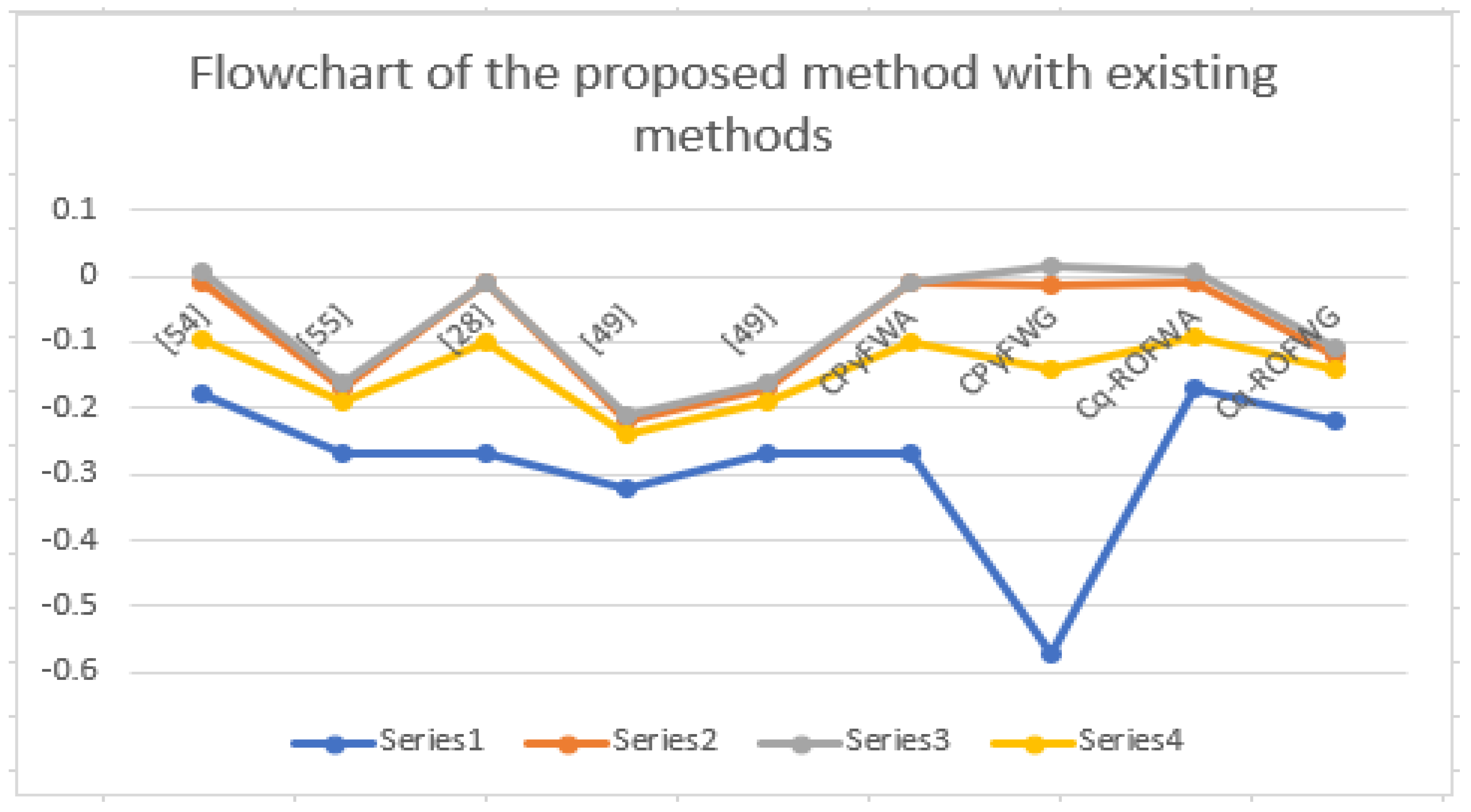
So, X 2 is the best company for investment. Notice that the both operators have provided different results. The Cq-ROFWA operator shows X 2 is a best candidate and X 1 is a last option, but the Cq-ROFGA operator shows X 2 is a best candidate and X 3 is a last option. The comparison of the proposed method with existing methods are discussed in Table 9.
The geometrical interpretation of the proposed work described in Table 9 are available in Figure 2.
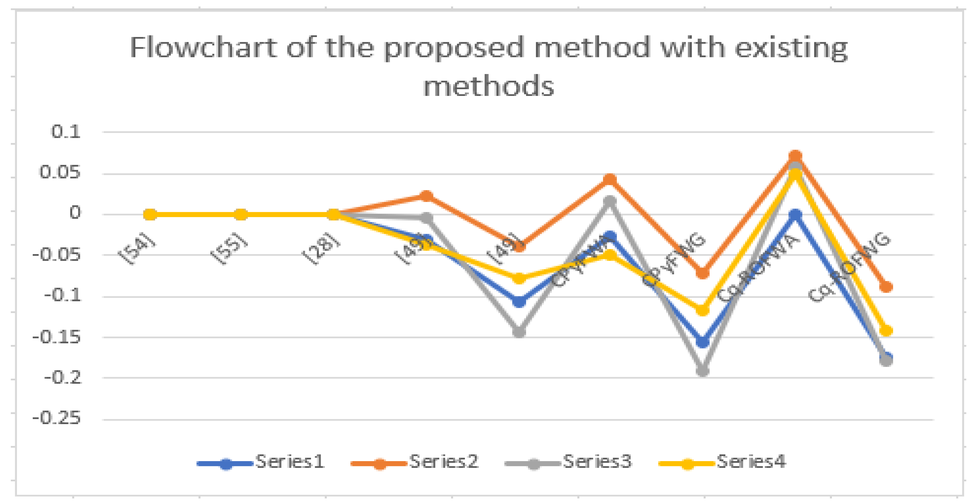
Firstly, we discuss some particular cases of the Cq-ROFWA operator by putting different values of parameter q , and the comparison between proposed method and existing works is given in Table 10.
The geometrical interpretation of the proposed work described in Table 10 are available in Figure 3.
It is clear that the existing methods and our proposed methods are provided that X 2 is the best candidate. However, the CIFS and CPyFS cannot describe the problems effectively, and the Cqq-ROFS is more powerful tool to deal with uncertain and unpredictable information in real decision making problems. For further discussion, we will check the superiority and flexibility of our proposed methods with the help of parameters q for different values. When we considered the Cq-ROFS types, the CIFS and CPyFS cannot describe it. The condition of CIFS and CPyFS is not satisfied effectively. When we provided the complex q-rung orthopair fuzzy kinds of information to CPyFs, they are given the results but not holds the condition of CPyFS, because the data is complex q-rung orthopair fuzzy types.
The comparisons between Cq-ROFWA and Cq-ROFWG operators are given in Table 11 and Table 12.
The advantages of the proposed methods are given by compared with existing methods.
(1)
The proposed method assumes that the sum of q-power of membership and q-power of non-membership grade is restricted to unit disc in complex plane. When a decision maker provides such kind of information like ( ( 0.9 ) . e i . 2 π ( 0.76 ) , ( 0.78 ) . e i . 2 π ( 0.72 ) ) , then the CIFS and CPyFS is not able to handle it. The notion of Cq-ROFS is able to handle this kind of sanitations. The constraint of Cq-ROFS is that the sum of q-power of membership and q-power of non-membership grade is restricted to unit disc in complex plane.
(2)
The proposed methods are more general than CIFS and CPyFS. The notion of CIFS and CPyFS all are the special cases of our proposed method. When, we will consider q = 1 , then the proposed work is reduced to CIFS. When, we will consider q = 2 , then the proposed work is reduced to CPyFS. The Cq-ROFS is more superior than CIF and CPyFS.
From the above comparisons, it is clear that the proposed methods in this paper such as Cq-ROFWA and Cq-ROFWG operators are more general than CIFS and CPyFS. Therefore, the proposed methods in this manuscript are more suitable to solve the MAGDM problems.

6. Conclusions

The aims of this article, the notion of q-rung orthopair fuzzy sets (q-ROFSs) and complex fuzzy sets (CFSs) are combined is to propose the novel approach of complex q-rung orthopair fuzzy sets (Cq-ROFSs) and their fundamental laws. The Cq-ROFSs are an important way to express uncertain information, and they are superior to the complex intuitionistic fuzzy sets and the complex Pythagorean fuzzy sets. Their eminent characteristic is that the sum of the qth power of the real part (similarly for imaginary part) of complex-valued membership degree and the qth power of the real part (similarly for imaginary part) of complex-valued non-membership degree is equal to or less than 1, so the space of uncertain information they can describe is broader. Based on these advantages, we proposed the Cq-ROFWA and Cq-ROFGA operators and studied their results with examples. Furthermore, we investigated some methods based on these operators to solve the MADM problems. Finally, we used the weighted averaging and geometric operators to illustrated the reliability and superiority of the proposed work and also discussed the advantages of the proposed work by compared with the other existing work. The comparison of the proposed method with existing methods are also discussed in this manuscript.

Author Contributions

Conceptualization, Z.A., T.M.; Data curation, P.L. and T.M.; Formal analysis, P.L. Z.A.; Funding acquisition, P.L.; Investigation, P.L. and T.M.; Methodology, P.L., T.M. and Z.A.; Resources, T.M.; Software, T.M.; Supervision, T.M. and P.L.; Writing—original draft, Z.A.; Writing—review & editing, P.L. and T.M. All authors have read and agreed to the published version of the manuscript.

Funding

This paper is supported by the National Natural Science Foundation of China (Nos. 71771140 and 71471172), Project of cultural masters and “the four kinds of a batch” talents, the Special Funds of Taishan Scholars Project of Shandong Province (No. ts201511045).

Conflicts of Interest

The authors declare no conflicts of interest.

References

  1. Zadeh, L.A. Fuzzy sets. Inf. Control 1965, 8, 338–353. [Google Scholar] [CrossRef] [Green Version]
  2. Zadeh, L.A. The concept of a linguistic variable and its application to approximate reasoning—I. Inf. Sci. 1975, 8, 199–249. [Google Scholar] [CrossRef]
  3. Coupland, S.; John, R. Geometric type-1 and type-2 fuzzy logic systems. IEEE Trans. Fuzzy Syst. 2007, 15, 3–15. [Google Scholar] [CrossRef]
  4. Atanassov, K.T. Intuitionistic fuzzy sets. In Intuitionistic Fuzzy Sets; Physica: Heidelberg, Germany, 1999; pp. 1–137. [Google Scholar]
  5. Vlachos, I.K.; Sergiadis, G.D. Intuitionistic fuzzy information–applications to pattern recognition. Pattern Recognit. Lett. 2007, 28, 197–206. [Google Scholar] [CrossRef]
  6. Xu, Z.; Yager, R.R. Dynamic intuitionistic fuzzy multi-attribute decision making. Int. J. Approx. Reason. 2008, 48, 246–262. [Google Scholar] [CrossRef] [Green Version]
  7. Wei, G. Some induced geometric aggregation operators with intuitionistic fuzzy information and their application to group decision making. Appl. Soft Comput. 2010, 10, 423–431. [Google Scholar] [CrossRef]
  8. Tan, C.; Chen, X. Intuitionistic fuzzy Choquet integral operator for multi-criteria decision making. Expert Syst. Appl. 2010, 37, 149–157. [Google Scholar] [CrossRef]
  9. Zhao, X.; Wei, G. Some intuitionistic fuzzy Einstein hybrid aggregation operators and their application to multiple attribute decision making. Knowl.-Based Syst. 2013, 37, 472–479. [Google Scholar] [CrossRef]
  10. Wei, G.; Zhao, X. Some induced correlated aggregating operators with intuitionistic fuzzy information and their application to multiple attribute group decision making. Expert Syst. Appl. 2012, 39, 2026–2034. [Google Scholar] [CrossRef]
  11. Kahraman, C.; Keshavarz Ghorabaee, M.; Zavadskas, E.K.; Cevik Onar, S.; Yazdani, M.; Oztaysi, B. Intuitionistic fuzzy EDAS method: An application to solid waste disposal site selection. J. Environ. Eng. Landsc. Manag. 2017, 25, 1–12. [Google Scholar] [CrossRef]
  12. Bolturk, E.; Kahraman, C. Interval-valued intuitionistic fuzzy CODAS method and its application to wave energy facility location selection problem. J. Intell. Fuzzy Syst. 2018, 35, 4865–4877. [Google Scholar] [CrossRef]
  13. Jiang, W.; Wei, B.; Liu, X.; Li, X.; Zheng, H. Intuitionistic fuzzy power aggregation operator based on entropy and its application in decision making. Int. J. Intell. Syst. 2018, 33, 49–67. [Google Scholar] [CrossRef]
  14. Yeni, F.B.; Özçelik, G. Interval-valued Atanassov intuitionistic Fuzzy CODAS method for multi criteria group decision making problems. Group Decis. Negot. 2019, 28, 433–452. [Google Scholar] [CrossRef]
  15. Li, Y.; Olson, D.L.; Qin, Z. Similarity measures between intuitionistic fuzzy (vague) sets: A comparative analysis. Pattern Recognit. Lett. 2007, 28, 278–285. [Google Scholar] [CrossRef]
  16. Yager, R.R. Pythagorean fuzzy subsets. In Proceedings of the 2013 Joint IFSA World Congress and NAFIPS Annual Meeting (IFSA/NAFIPS), Edmonton, AB, Canada, 24 June 2013; pp. 57–61. [Google Scholar]
  17. Zhang, X.; Xu, Z. Extension of TOPSIS to multiple criteria decision making with Pythagorean fuzzy sets. Int. J. Intell. Syst. 2014, 29, 1061–1078. [Google Scholar] [CrossRef]
  18. Mete, S. Assessing occupational risks in pipeline construction using FMEA-based AHP-MOORA integrated approach under Pythagorean fuzzy environment. Hum. Ecol. Risk Assess. Int. J. 2018, 25, 1645–1660. [Google Scholar] [CrossRef]
  19. Yang, Y.; Ding, H.; Chen, Z.S.; Li, Y.L. A note on extension of TOPSIS to multiple criteria decision making with Pythagorean fuzzy sets. Int. J. Intell. Syst. 2016, 31, 68–72. [Google Scholar] [CrossRef]
  20. Garg, H. A new generalized Pythagorean fuzzy information aggregation using Einstein operations and its application to decision making. Int. J. Intell. Syst. 2016, 31, 886–920. [Google Scholar] [CrossRef]
  21. Peng, X.; Yang, Y. Pythagorean fuzzy Choquet integral based MABAC method for multiple attribute group decision making. Int. J. Intell. Syst. 2016, 31, 989–1020. [Google Scholar] [CrossRef]
  22. Garg, H. Generalized Pythagorean fuzzy geometric aggregation operators using Einstein t-norm and t-conorm for multicriteria decision-making process. Int. J. Intell. Syst. 2017, 32, 597–630. [Google Scholar] [CrossRef]
  23. Verma, R.; Merigó, J.M. On generalized similarity measures for Pythagorean fuzzy sets and their applications to multiple attribute decision-making. Int. J. Intell. Syst. 2019, 34, 2556–2583. [Google Scholar] [CrossRef]
  24. Peng, X.; Li, W. Algorithms for interval-valued pythagorean fuzzy sets in emergency decision making based on multiparametric similarity measures and WDBA. IEEE Access 2019, 7, 7419–7441. [Google Scholar] [CrossRef]
  25. Zhou, F.; Chen, T.Y. A Novel Distance Measure for Pythagorean Fuzzy Sets and its Applications to the Technique for Order Preference by Similarity to Ideal Solutions. Int. J. Comput. Intell. Syst. 2019, 12, 955–969. [Google Scholar] [CrossRef] [Green Version]
  26. Khan, A.A.; Ashraf, S.; Abdullah, S.; Qiyas, M.; Luo, J.; Khan, S.U. Pythagorean fuzzy Dombi aggregation operators and their application in decision support system. Symmetry 2019, 11, 383. [Google Scholar] [CrossRef] [Green Version]
  27. Yager, R.R. Generalized orthopair fuzzy sets. IEEE Trans. Fuzzy Syst. 2017, 25, 1222–1230. [Google Scholar] [CrossRef]
  28. Liu, P.; Wang, P. Some q-rung orthopair fuzzy aggregation operators and their applications to multiple-attribute decision making. Int. J. Intell. Syst. 2018, 33, 259–280. [Google Scholar] [CrossRef]
  29. Liu, P.; Liu, J. Some q-rung orthopai fuzzy Bonferroni mean operators and their application to multi-attribute group decision making. Int. J. Intell. Syst. 2018, 33, 315–347. [Google Scholar] [CrossRef]
  30. Peng, X.; Dai, J.; Garg, H. Exponential operation and aggregation operator for q-rung orthopair fuzzy set and their decision-making method with a new score function. Int. J. Intell. Syst. 2018, 33, 2255–2282. [Google Scholar] [CrossRef]
  31. Wei, G.; Gao, H.; Wei, Y. Some q-rung orthopair fuzzy Heronian mean operators in multiple attribute decision making. Int. J. Intell. Syst. 2018, 33, 1426–1458. [Google Scholar] [CrossRef]
  32. Liu, P.; Wang, P. Multiple-attribute decision making based on Archimedean Bonferroni operators of q-rung orthopair fuzzy numbers. IEEE Trans. Fuzzy Syst. 2018, 27, 834–848. [Google Scholar] [CrossRef]
  33. Liu, Z.; Liu, P.; Liang, X. Multiple attribute decision-making method for dealing with heterogeneous relationship among attributes and unknown attribute weight information under q-rung orthopair fuzzy environment. Int. J. Intell. Syst. 2018, 33, 1900–1928. [Google Scholar] [CrossRef]
  34. Du, W.S. Minkowski-type distance measures for generalized orthopair fuzzy sets. Int. J. Intell. Syst. 2018, 33, 802–817. [Google Scholar] [CrossRef]
  35. Ali, M.I. Another view on q-rung orthopair fuzzy sets. Int. J. Intell. Syst. 2018, 33, 2139–2153. [Google Scholar] [CrossRef]
  36. Liu, P.; Chen, S.M.; Wang, P. Multiple-attribute group decision-making based on q-rung orthopair fuzzy power maclaurin symmetric mean operators. IEEE Trans. Syst. Man Cybern. Syst. 2018, 1–16. [Google Scholar] [CrossRef]
  37. Yager, R.R.; Alajlan, N.; Bazi, Y. Aspects of generalized orthopair fuzzy sets. Int. J. Intell. Syst. 2018, 33, 2154–2174. [Google Scholar] [CrossRef]
  38. Ramot, D.; Milo, R.; Friedman, M.; Kandel, A. Complex fuzzy sets. IEEE Trans. Fuzzy Syst. 2002, 10, 171–186. [Google Scholar] [CrossRef]
  39. Buckley, J.J. Fuzzy Complex Numbers. Fuzzy Sets Syst. 1989, 33, 333–345. [Google Scholar] [CrossRef]
  40. Nguyen, H.T.; Kandel, A.; Kreinovich, V. Complex Fuzzy Sets: Towards New Foundations. In Proceedings of the Ninth IEEE International Conference on Fuzzy Systems. FUZZ-IEEE 2000 (Cat. No. 00CH37063), San Antonio, TX, USA, 7–10 May 2000; Volume 2, pp. 1045–1048. [Google Scholar]
  41. Zhang, G.; Dillon, T.S.; Cai, K.Y.; Ma, J.; Lu, J. Operation properties and δ-equalities of complex fuzzy sets. Int. J. Approx. Reason. 2009, 50, 1227–1249. [Google Scholar] [CrossRef] [Green Version]
  42. Alkouri, A.M.; Salleh, A.R. Complex intuitionistic fuzzy sets. AIP Conf. Proc. 2012, 1482, 464–470. [Google Scholar]
  43. Kumar, T.; Bajaj, R.K. On complex intuitionistic fuzzy soft sets with distance measures and entropies. J. Math. 2014. [Google Scholar] [CrossRef] [Green Version]
  44. Quek, S.G.; Selvachandran, G.; Davvaz, B.; Pal, M. The algebraic structures of complex intuitionistic fuzzy soft sets associated with groups and subgroups. Sci. Iran. 2019, 26, 1898–1912. [Google Scholar] [CrossRef] [Green Version]
  45. Al-Qudah, Y.; Hassan, N. Complex multi-fuzzy soft expert set and its application. Int. J. Math. Comput. Sci. 2019, 14, 149–176. [Google Scholar]
  46. Roy, S.; Samanta, T.K. A note on fuzzy soft topological spaces. Ann. Fuzzy Math. Inform. 2012, 3, 305–311. [Google Scholar]
  47. Al-Qudah, Y.; Hassan, N. Complex multi-fuzzy soft set: Its entropy and similarity measure. IEEE Access 2018, 6, 65002–65017. [Google Scholar] [CrossRef]
  48. Liu, P.; Ali, Z.; Mahmood, T. A Method to Multi-Attribute Group Decision-Making Problem with Complex q-Rung Orthopair Linguistic Information Based on Heronian Mean Operators. Int. J. Comput. Intell. Syst. 2018, 33, 315–347. [Google Scholar] [CrossRef]
  49. Garg, H.; Rani, D. Some generalized complex intuitionistic fuzzy aggregation operators and their application to multicriteria decision-making process. Arab. J. Sci. Eng. 2019, 44, 2679–2698. [Google Scholar] [CrossRef]
  50. Garg, H.; Rani, D. A robust correlation coefficient measure of complex intuitionistic fuzzy sets and their applications in decision-making. Appl. Intell. 2019, 49, 496–512. [Google Scholar] [CrossRef]
  51. Rani, D.; Garg, H. Complex intuitionistic fuzzy power aggregation operators and their applications in multicriteria decision-making. Expert Syst. 2018, 35, e12325. [Google Scholar] [CrossRef]
  52. Ullah, K.; Mahmood, T.; Ali, Z.; Jan, N. On some distance measures of complex Pythagorean fuzzy sets and their applications in pattern recognition. Complex. Intell. Syst. 2019, 1–13. [Google Scholar] [CrossRef] [Green Version]
  53. Akram, M.; Naz, S. A novel decision-making approach under complex Pythagorean fuzzy environment. Math. Comput. Appl. 2019, 24, 73. [Google Scholar] [CrossRef] [Green Version]
  54. Xu, Z. Intuitionistic fuzzy aggregation operators. IEEE Trans. Fuzzy Syst. 2007, 15, 1179–1187. [Google Scholar]
  55. Garg, H. Confidence levels based Pythagorean fuzzy aggregation operators and its application to decision-making process. Comput. Math. Organ. Theory 2017, 23, 546–571. [Google Scholar] [CrossRef]
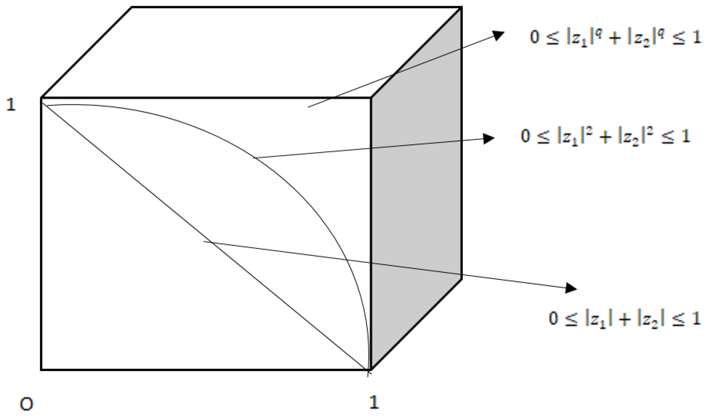
Figure 1. Comparisons of restrictions of complex intuitionistic fuzzy set (CIFS), complex pythagorean fuzzy set (CPyFS), and complex q-rung orthopair fuzzy sets (Cq-ROFS).
Information 11 00005 g001
Figure 2. Graphical representation of the proposed methods and existing method discussed in Table 9.
Information 11 00005 g002
Figure 3. Graphical representation of the proposed methods and existing method discussed in Table 10.
Information 11 00005 g003
Table 1. The decision matrix D for Example 3.
C q R O F N s c 1 c 2 c 3 c 4
X 1 ( ( 0.8 ) . e i . 2 π ( 0.7 ) , ( 0.7 ) . e i . 2 π ( 0.8 ) ) ( ( 0.6 ) . e i . 2 π ( 0.9 ) , ( 0.9 ) . e i . 2 π ( 0.6 ) ) ( ( 0.5 ) . e i . 2 π ( 0.92 ) , ( 0.91 ) . e i . 2 π ( 0.5 ) ) ( ( 0.4 ) . e i . 2 π ( 0.4 ) , ( 0.7 ) . e i . 2 π ( 0.8 ) )
X 2 ( ( 0.7 ) . e i . 2 π ( 0.8 ) , ( 0.8 ) . e i . 2 π ( 0.9 ) ) ( ( 0.7 ) . e i . 2 π ( 0.6 ) , ( 0.7 ) . e i . 2 π ( 0.7 ) ) ( ( 0.87 ) . e i . 2 π ( 0.68 ) , ( 0.78 ) . e i . 2 π ( 0.77 ) ) ( ( 0.43 ) . e i . 2 π ( 0.85 ) , ( 0.91 ) . e i . 2 π ( 0.56 ) )
X 3 ( ( 0.7 ) . e i . 2 π ( 0.4 ) , ( 0.9 ) . e i . 2 π ( 0.6 ) ) ( ( 0.4 ) . e i . 2 π ( 0.4 ) , ( 0.7 ) . e i . 2 π ( 0.8 ) ) ( ( 0.45 ) . e i . 2 π ( 0.77 ) , ( 0.76 ) . e i . 2 π ( 0.61 ) ) ( ( 0.72 ) . e i . 2 π ( 0.87 ) , ( 0.84 ) . e i . 2 π ( 0.47 ) )
X 4 ( ( 0.9 ) . e i . 2 π ( 0.5 ) , ( 0.7 ) . e i . 2 π ( 0.6 ) ) ( ( 0.6 ) . e i . 2 π ( 0.8 ) , ( 0.83 ) . e i . 2 π ( 0.74 ) ) ( ( 0.72 ) . e i . 2 π ( 0.64 ) , ( 0.55 ) . e i . 2 π ( 0.69 ) ) ( ( 0.67 ) . e i . 2 π ( 0.58 ) , ( 0.68 ) . e i . 2 π ( 0.67 ) )
Table 2. The normalized matrix.
C q R O F N s c 1 c 2 c 3 c 4
X 1 ( ( 0.7 ) . e i . 2 π ( 0.8 ) , ( 0.8 ) . e i . 2 π ( 0.7 ) ) ( ( 0.6 ) . e i . 2 π ( 0.9 ) , ( 0.9 ) . e i . 2 π ( 0.6 ) ) ( ( 0.5 ) . e i . 2 π ( 0.92 ) , ( 0.91 ) . e i . 2 π ( 0.5 ) ) ( ( 0.4 ) . e i . 2 π ( 0.4 ) , ( 0.7 ) . e i . 2 π ( 0.8 ) )
X 2 ( ( 0.8 ) . e i . 2 π ( 0.9 ) , ( 0.7 ) . e i . 2 π ( 0.8 ) ) ( ( 0.7 ) . e i . 2 π ( 0.6 ) , ( 0.7 ) . e i . 2 π ( 0.7 ) ) ( ( 0.87 ) . e i . 2 π ( 0.68 ) , ( 0.78 ) . e i . 2 π ( 0.77 ) ) ( ( 0.43 ) . e i . 2 π ( 0.85 ) , ( 0.91 ) . e i . 2 π ( 0.56 ) )
X 3 ( ( 0.9 ) . e i . 2 π ( 0.6 ) , ( 0.7 ) . e i . 2 π ( 0.4 ) ) ( ( 0.4 ) . e i . 2 π ( 0.4 ) , ( 0.7 ) . e i . 2 π ( 0.8 ) ) ( ( 0.45 ) . e i . 2 π ( 0.77 ) , ( 0.76 ) . e i . 2 π ( 0.61 ) ) ( ( 0.72 ) . e i . 2 π ( 0.87 ) , ( 0.84 ) . e i . 2 π ( 0.47 ) )
X 4 ( ( 0.7 ) . e i . 2 π ( 0.6 ) , ( 0.9 ) . e i . 2 π ( 0.5 ) ) ( ( 0.6 ) . e i . 2 π ( 0.8 ) , ( 0.83 ) . e i . 2 π ( 0.74 ) ) ( ( 0.72 ) . e i . 2 π ( 0.64 ) , ( 0.55 ) . e i . 2 π ( 0.69 ) ) ( ( 0.67 ) . e i . 2 π ( 0.58 ) , ( 0.68 ) . e i . 2 π ( 0.67 ) )
Table 3. The overall value of each alternative by the Cq-ROFWA operator.
Alternatives C q R O F W A
X 1 ( ( 0.60 ) . e i . 2 π ( 0.85 ) , ( 0.83 ) . e i . 2 π ( 0.65 ) )
X 2 ( ( 0.74 ) . e i . 2 π ( 0.79 ) , ( 0.75 ) . e i . 2 π ( 0.70 ) )
X 3 ( ( 0.74 ) . e i . 2 π ( 0.69 ) , ( 0.73 ) . e i . 2 π ( 0.59 ) )
X 4 ( ( 0.66 ) . e i . 2 π ( 0.72 ) , ( 0.78 ) . e i . 2 π ( 0.65 ) )
Table 4. The overall value of each alternative by the Cq-ROFWG operator.
Alternatives C q R O F W G
X 1 ( ( 0.57 ) . e i . 2 π ( 0.75 ) , ( 0.86 ) . e i . 2 π ( 0.68 ) )
X 2 ( ( 0.67 ) . e i . 2 π ( 0.72 ) , ( 0.78 ) . e i . 2 π ( 0.72 ) )
X 3 ( ( 0.56 ) . e i . 2 π ( 0.55 ) , ( 0.75 ) . e i . 2 π ( 0.70 ) )
X 4 ( ( 0.65 ) . e i . 2 π ( 0.68 ) , ( 0.82 ) . e i . 2 π ( 0.68 ) )
Table 5. The normalized matrix.
C q R O F N s c 1 c 2 c 3 c 4
X 1 ( 0.40 , 0.30 ) ( 0.50 , 0.40 ) ( 0.42 , 0.32 ) ( 0.52 , 0.42 )
X 2 ( 0.41 , 0.31 ) ( 0.51 , 0.41 ) ( 0.43 , 0.33 ) ( 0.53 , 0.43 )
X 3 ( 0.42 , 0.32 ) ( 0.52 , 0.42 ) ( 0.40 , 0.30 ) ( 0.50 , 0.40 )
X 4 ( 0.43 , 0.33 ) ( 0.53 , 0.43 ) ( 0.41 , 0.31 ) ( 0.51 , 0.41 )
Table 6. The normalized matrix.
C q R O F N s c 1 c 2 c 3 c 4
X 1 ( 0.40 e i . 2 π ( 0.0 ) , 0.30 e i . 2 π ( 0.0 ) ) ( 0.50 e i . 2 π ( 0.0 ) , 0.40 e i . 2 π ( 0.0 ) ) ( 0.42 e i . 2 π ( 0.0 ) , 0.32 e i . 2 π ( 0.0 ) ) ( 0.52 e i . 2 π ( 0.0 ) , 0.42 e i . 2 π ( 0.0 ) )
X 2 ( 0.41 e i . 2 π ( 0.0 ) , 0.31 e i . 2 π ( 0.0 ) ) ( 0.51 e i . 2 π ( 0.0 ) , 0.41 e i . 2 π ( 0.0 ) ) ( 0.43 e i . 2 π ( 0.0 ) , 0.33 e i . 2 π ( 0.0 ) ) ( 0.53 e i . 2 π ( 0.0 ) , 0.43 e i . 2 π ( 0.0 ) )
X 3 ( 0.42 e i . 2 π ( 0.0 ) , 0.32 e i . 2 π ( 0.0 ) ) ( 0.52 e i . 2 π ( 0.0 ) , 0.42 e i . 2 π ( 0.0 ) ) ( 0.40 e i . 2 π ( 0.0 ) , 0.30 e i . 2 π ( 0.0 ) ) ( 0.50 e i . 2 π ( 0.0 ) , 0.40 e i . 2 π ( 0.0 ) )
X 4 ( 0.43 e i . 2 π ( 0.0 ) , 0.33 e i . 2 π ( 0.0 ) ) ( 0.53 e i . 2 π ( 0.0 ) , 0.43 e i . 2 π ( 0.0 ) ) ( 0.41 e i . 2 π ( 0.0 ) , 0.31 e i . 2 π ( 0.0 ) ) ( 0.51 e i . 2 π ( 0.0 ) , 0.41 e i . 2 π ( 0.0 ) )
Table 7. The overall value of each alternative by the complex q-rung orthopair fuzzy weighted averaging (Cq-ROFWA) operator.
Alternatives C q R O F W A
X 1 ( 0.60 , 0.83 ) = ( 0.60 e i . 2 π ( 0.0 ) , 0.83 e i . 2 π ( 0.0 ) )
X 2 ( 0.74 , 0.75 ) = ( 0.74 e i . 2 π ( 0.0 ) , 0.75 e i . 2 π ( 0.0 ) )
X 3 ( 0.74 , 0.73 ) = ( 0.74 e i . 2 π ( 0.0 ) , 0.73 e i . 2 π ( 0.0 ) )
X 4 ( 0.66 , 0.78 ) = ( 0.66 e i . 2 π ( 0.0 ) , 0.78 e i . 2 π ( 0.0 ) )
Table 8. The overall value of each alternative by the complex q-rung orthopair fuzzy weighted geometric operator (Cq-ROFWG) operator.
Alternatives C q R O F W G
X 1 ( 0.57 , 0.86 ) = ( 0.57 e i . 2 π ( 0.0 ) , 0.86 e i . 2 π ( 0.0 ) )
X 2 ( 0.67 , 0.78 ) = ( 0.67 e i . 2 π ( 0.0 ) , 0.78 e i . 2 π ( 0.0 ) )
X 3 ( 0.56 , 0.75 ) = ( 0.56 e i . 2 π ( 0.0 ) , 0.75 e i . 2 π ( 0.0 ) )
X 4 ( 0.65 , 0.82 ) = ( 0.65 e i . 2 π ( 0.0 ) , 0.82 e i . 2 π ( 0.0 ) )
Table 9. Comparison between proposed method with existing methods for Example 4.
M e t h o d s . Score ValuesRanking Results
Xu [54] S ( X 1 ) = 0.18 ,
S ( X 2 ) = 0.0085 ,
S ( X 3 ) = 0.00804 ,
S ( X 4 ) = 0.094
X 1 X 4 X 2 X 3
Garg [55] S ( X 1 ) = 0.27 ,
S ( X 2 ) = 0.17 ,
S ( X 3 ) = 0.16 ,
S ( X 4 ) = 0.19
X 1 X 4 X 2 X 3
Liu and Wang [28] S ( X 1 ) = 0.27 ,
S ( X 2 ) = 0.0093 ,
S ( X 3 ) = 0.00894 ,
S ( X 4 ) = 0.1
X 1 X 4 X 2 X 3
Garg and Rani [49] CIFWA S ( X 1 ) = 0.32 ,
S ( X 2 ) = 0.22 ,
S ( X 3 ) = 0.21 ,
S ( X 4 ) = 0.24
X 1 X 4 X 2 X 3
Garg and Rani [49] CIFWG S ( X 1 ) = 0.27 ,
S ( X 2 ) = 0.17 ,
S ( X 3 ) = 0.16 ,
S ( X 4 ) = 0.19
X 1 X 4 X 2 X 3
Exiting work CPyFWA S ( X 1 ) = 0.27 ,
S ( X 2 ) = 0.0093 ,
S ( X 3 ) = 0.00894 ,
S ( X 4 ) = 0.1
X 1 X 4 X 2 X 3
Existing work CPyFWG S ( X 1 ) = 0.57 ,
S ( X 2 ) = 0.0133 ,
S ( X 3 ) = 0.01294 ,
S ( X 4 ) = 0.14
X 1 X 4 X 2 X 3
Proposed work in this article Cq-ROFWA S ( X 1 ) = 0.17 ,
S ( X 2 ) = 0.0083 ,
S ( X 3 ) = 0.00794 ,
S ( X 4 ) = 0.09
X 1 X 4 X 2 X 3
Proposed work in this article Cq-ROFWG S ( X 1 ) = 0.22 ,
S ( X 2 ) = 0.12 ,
S ( X 3 ) = 0.11 ,
S ( X 4 ) = 0.14
X 1 X 4 X 2 X 3
Table 10. Ranking results between different existing works for Example 3.
MethodsScore ValuesRanking
Xu [54] Cannot   be   Calculated Cannot   be   Calculated
Garg [55] Cannot   be   Calculated Cannot   be   Calculated
Liu and Wang [28] Cannot   be   Calculated Cannot   be   Calculated
Garg and Rani [49] CIFWA S ( X 1 ) = 0.0299 ,
S ( X 2 ) = 0.0223 ,
S ( X 3 ) = 0.00487 ,
S ( X 4 ) = 0.0362
X 4 X 1 X 3 X 2
Garg and Rani [49] CIFWG S ( X 1 ) = 0.106 ,
S ( X 2 ) = 0.04 ,
S ( X 3 ) = 0.144 ,
S ( X 4 ) = 0.077
X 3 X 1 X 4 X 2
Exiting work CPyFWA S ( X 1 ) = 0.0276 ,
S ( X 2 ) = 0.043 ,
S ( X 3 ) = 0.016 ,
S ( X 4 ) = 0.050
X 4 X 1 X 3 X 2
Existing work CPyFWG S ( X 1 ) = 0.1551 ,
S ( X 3 ) = 0.19 ,
S ( X 4 ) = 0.117
X 3 X 1 X 4 X 2
Proposed work in this article Cq-ROFWA S ( X 1 ) = 0.0007 ,
S ( X 2 ) = 0.071 ,
S ( X 3 ) = 0.057 ,
S ( X 4 ) = 0.049
X 1 X 4 X 3 X 2
Proposed work in this article Cq-ROFWG S ( X 1 ) = 0.174 ,
S ( X 2 ) = 0.0878 ,
S ( X 3 ) = 0.178 ,
S ( X 4 ) = 0.142
X 3 X 1 X 4 X 2
Table 11. The overall value of each alternative by the Cq-ROFWA operator for different values of parameters q .
RequirementsMethodsScore ValuesRanking
Xu [54] Cannot   be   Calculated Cannot   be   Calculated Cannot   be   Calculated
Garg [55] Cannot   be   Calculated Cannot   be   Calculated Cannot   be   Calculated
Liu and Wang [28] Cannot   be   Calculated Cannot   be   Calculated Cannot   be   Calculated
C I F S = a b l e
C P y F S = a b l e
q R O F S = able
q = 1 S ( X 1 ) = 0.0299 ,
S ( X 2 ) = 0.0223 ,
S ( X 3 ) = 0.00487 ,
S ( X 4 ) = 0.0362
X 4 X 1 X 3 X 2
C I F S = n o t   a b l e
C P y F S = a b l e
C q R O F S = a b l e
q = 2 S ( X 1 ) = 0.0276 ,
S ( X 2 ) = 0.043 ,
S ( X 3 ) = 0.016 ,
S ( X 4 ) = 0.050
X 4 X 1 X 3 X 2
C I F S = n o t   a b l e
C P y F S = n o t   a b l e
C q R O F S = a b l e
q = 4 S ( X 1 ) = 0.0007 ,
S ( X 2 ) = 0.071 ,
S ( X 3 ) = 0.057 ,
S ( X 4 ) = 0.049
X 1 X 4 X 3 X 2
C I F S = n o t   a b l e
C P y F S = n o t   a b l e
C q R O F S = a b l e
q = 8 S ( X 1 ) = 0.036 ,
S ( X 2 ) = 0.0744 ,
S ( X 3 ) = 0.070 ,
S ( X 4 ) = 0.022
X 4 X 1 X 3 X 2
C I F S = n o t   a b l e
C P y F S = n o t   a b l e
C q R O F S = a b l e
q = 15 S ( X 1 ) = 0.036 ,
S ( X 2 ) = 0.040 ,
S ( X 3 ) = 0.037 ,
S ( X 4 ) = 0.0036
X 4 X 1 X 3 X 2
C I F S = n o t   a b l e
C P y F S = n o t   a b l e
C q R O F S = a b l e
q = 16 S ( X 1 ) = 0.034 ,
S ( X 2 ) = 0.036 ,
S ( X 3 ) = 0.033 ,
S ( X 4 ) = 0.002
X 4 X 1 X 3 X 2
Table 12. The overall value of each alternative by the Cq-ROFWG operator for different values of parameter q .
RequirementsMethodsScore ValuesRanking
Xu [54] Cannot   be   Calculated Cannot   be   Calculated Cannot   be   Calculated
Garg [55] Cannot   be   Calculated Cannot   be   Calculated Cannot   be   Calculated
Liu and Wang [28] Cannot   be   Calculated Cannot   be   Calculated Cannot   be   Calculated
C I F S = a b l e
C P y F S = a b l e
C q R O F S = a b l e
q = 1 S ( X 1 ) = 0.106 ,
S ( X 2 ) = 0.04 ,
S ( X 3 ) = 0.144 ,
S ( X 4 ) = 0.077
X 3 X 1 X 4 X 2
C I F S = n o t   a b l e
C P y F S = a b l e
C q R O F S = a b l e
q = 2 S ( X 1 ) = 0.1551 ,
S ( X 2 ) = 0.0727 ,
S ( X 3 ) = 0.19 ,
S ( X 4 ) = 0.117
X 3 X 1 X 4 X 2
C I F S = n o t   a b l e
C P y F S = n o t   a b l e
C q R O F S = a b l e
q = 4 S ( X 1 ) = 0.174 ,
S ( X 2 ) = 0.0878 ,
S ( X 3 ) = 0.178 ,
S ( X 4 ) = 0.142
X 3 X 1 X 4 X 2
C I F S = n o t   a b l e
C P y F S = n o t   a b l e
C q R O F S = a b l e
q = 8 S ( X 1 ) = 0.13 ,
S ( X 2 ) = 0.068 ,
S ( X 3 ) = 0.084 ,
S ( X 4 ) = 0.10
X 1 X 4 X 3 X 2
C I F S = n o t   a b l e
C P y F S = n o t   a b l e
C q R O F S = a b l e
q = 15 S ( X 1 ) = 0.064 ,
S ( X 2 ) = 0.031 ,
S ( X 3 ) = 0.017 ,
S ( X 4 ) = 0.042
X 1 X 4 X 2 X 3
C I F S = n o t   a b l e
C P y F S = n o t   a b l e
C q R O F S = a b l e
q = 16 S ( X 1 ) = 0.057 ,
S ( X 2 ) = 0.027 ,
S ( X 3 ) = 0.014 ,
S ( X 4 ) = 0.0367
X 1 X 4 X 2 X 3