Article

A Fast Method for Estimating the Number of Clusters Based on Score and the Minimum Distance of the Center Point

College of Computer Science and Technology, Henan Polytechnic University, Jiaozuo 454003, China
*
Author to whom correspondence should be addressed.
Information 2020, 11(1), 16; https://doi.org/10.3390/info11010016
Submission received: 25 November 2019 / Revised: 17 December 2019 / Accepted: 19 December 2019 / Published: 25 December 2019
(This article belongs to the Special Issue Big Data Integration)

Abstract

:
Clustering is widely used as an unsupervised learning algorithm. However, it is often necessary to manually enter the number of clusters, and the number of clusters has a great impact on the clustering effect. At present, researchers propose some algorithms to determine the number of clusters, but the results are not very good for determining the number of clusters of data sets with complex and scattered shapes. To solve these problems, this paper proposes using the Gaussian Kernel density estimation function to determine the maximum number of clusters, use the change of center point score to get the candidate set of center points, and further use the change of the minimum distance between center points to get the number of clusters. The experiment shows the validity and practicability of the proposed algorithm.

1. Introduction

Clustering analysis has a long history and is a key technology of data analysis. As an unsupervised learning algorithm [1], it does not require prior knowledge and has been widely applied to image processing, business intelligence, network mining, and other fields [2,3]. A clustering algorithm is used to divide data into multiple clusters and make the elements within clusters as similar as possible and the elements between clusters as different as possible.
At present, researchers propose a large number of clustering algorithms, including k-means algorithm based on partition, which is widely used because of its simplicity and rapidity. There is a DBSCAN algorithm based on density, which can recognize various shapes in the presence of noise. There are DPC [4] and LPC [5] algorithms based on density peak, which can quickly identify various shapes. Among the above algorithms, only DBSCAN algorithm does not need to input the number of clusters, while other algorithms need to input the number of clusters artificially. Moreover, the DBSCAN algorithm is also faced with the need to select the parameters when determining the number of clusters, and the clustering speed is slow. In practical applications, the number of clusters is determined according to people’s background knowledge and decision graph, which may be larger or smaller due to people’s lack of background knowledge and visual error. In addition, the determination of the number of clusters has a great influence on the quality of the clustering. Therefore, it is very important to determine the optimal number of clusters. At present, researchers also propose some methods to determine the number of clusters, including methods based on validity indexes, such as Silhouette index [6], I-index [7], Xie-Beni index [8], DBI [9] and new Bayesian index [10]. It is better to estimate the number of clusters with clear boundaries, but the cluster number estimation for complexly distributed datasets tends to be poor and slow. There are methods based on a clustering algorithm, such as the I-nice algorithm based on Gaussian model [11] and an algorithm based on improved density [12], which are relatively slow in cluster number calculation.
To solve the existing problems, it is not very good for the determination of the number of clusters of complex data sets and the speed of determining the number of clusters. This paper proposes an algorithm based on the change of scores and the minimum distance between the centers to determine the number of clusters. The algorithm in this paper mainly studies the automatic determination of the cluster number of data sets with complex shapes and distributed dispersion. The dispersion here is that at least one dimension of data overlap is not particularly severe. It does not require artificial input of cluster numbers and has a fast speed. The algorithm in this paper firstly gets the number of density peaks on the larger dispersed dimension through the density estimation of one-dimensional Gaussian kernel to narrow the value range of K. Then it gets the center point through the score of the points, and gets the candidate set of the center point according to the change of the score. In the candidate set, it gets the value of K according to the change of the distance of the center point. In the experimental part, the results of the proposed algorithm are compared and discussed with those of the proposed 11 typical algorithms on artificial data sets and real data sets.

2. Related Work

At present, researchers propose many methods for determining the number of clusters. For example, in 2014, Rodriguez and Laio [4] proposed clustering algorithms based on density peaks. Although the algorithm can handle non-spherical and strongly overlapping data sets, in fact, it cannot fully automate the determination of the number of clusters, requiring people to select the number of clusters according to the decision map. Next, the related techniques for determining the optimal number of clusters is summarized as follows. Existing algorithms can be roughly divided into two categories: one is based on validity index, and the other is based on existing clustering algorithms.
(1) Some methods determine the number of clusters based on clustering validity index. Davies and Bouldin proposed the DBI [9] in 1979. The DBI is based on the ratio between dispersion degree and distance between clusters to get the similarity between clusters, and the lowest similarity to get the best clustering number. In 2002, Ujjwal and Sanghamitra proposed a method to determine the number of clusters based on the validity index of I-index [7]. Xie and Beni proposed Xie-Beni index in 1991 [8]. This index is the ratio of intra-class compactness and inter-class separation. Xie-Beni index is also used to determine the optimal number of clusters. Bensaid et al. found that the size of each cluster had a great influence on Xie-Beni index, so they proposed an improved Xie-Beni index, which was no longer so sensitive to the number of elements. Min Ren et al. found that there was a problem with the improved index by Bensaid et al. When c n , the index will decrease monotonously, approaching 0, lacking the robustness to determine the optimal number of clusters. Therefore, Min Ren et al. proposed an improved Xie-Beni index [2] (Xie-Beni index with punitive measures) in 2016 to determine the optimal cluster number. Suneel proposed in 2018 to use diversity to determine the number of clusters [13], in other words, to encourage balanced clustering through cluster size and the distance between clusters. Zhou et al. proposed a validity index based on cluster centers and nearest neighbor clusters in 2018 [14], and used this index to determine the optimal number of clusters. Li et al. also proposed a new clustering validity index in 2019, which is based on the deviation ratio of the sum of squares and Euclidean distance [15], and designed a method to dynamically determine the optimal number based on the index. Ramazan and Petros [16] proposed in 2019 to assign weights to multiple clustering algorithms according to data sets and determine the number of clusters by using various indicators. Khan and Luo proposed an algorithm in 2019 to determine the number of clusters in fuzzy clustering by using variable weights [17], which introduced punishment rules and updated variable weights with formulas.
(2) Some classical clustering algorithms are used to determine the optimal number of clusters. Sugar and James [18] proposed a non-parametric method in 2003 that determined the number of clusters based on the average distance between each data sample and its nearest clustering center. Tong and Li et al. proposed the improved density algorithm scubi-dbscan algorithm [19] in 2017 to determine the cluster number while clustering. Zhou and Xu [20] proposed an algorithm to determine the number of clusters based on hierarchical clustering in 2017, and the number of clusters was obtained when a certain value was reached. Md Abdul Masud [11] proposed in 2018 to set up m observation points, calculate the distance between all data sets and these m points, establish m gaussian mixture models according to the distance data, and find the gaussian mixture model with the best fitting degree through AIC index. At this time, the number of components of the gaussian mixture model is the number of clusters. As there are always errors, Md Abdul Masud proposed that all the center points obtained by the established m gaussian mixture model should be combined with k-nearest neighbor calculation, and the number of the remaining center points should be the number of clusters. Avisek [21] proposed the maximum jump and final jump algorithm in 2018 to determine the optimal cluster number. Specifically, it uses the minimum distance change of the center point to obtain the number of clusters.
These algorithms are good at estimating the optimal number of clusters on a data set with a simple shape and a well-defined boundary. However, they are not particularly good for complex data sets and do not have good time performance. However, these algorithms broaden the way for us to further study the optimal cluster number of complex data sets.

3. Background

Density estimation can be divided into parametric estimation and nonparametric estimation. Kernel density estimation is a kind of non-parametric estimation algorithm, which obtains the characteristics of data distribution from the data itself, hardly requiring prior knowledge. The calculation formula of probability density function is shown in Formula (1). The commonly used kernel density estimation includes Gaussian Kernel function, Triangular Kernel function and Epanechniko Kernel function. The effects of these functions are similar, but in different forms. To present a smooth density curve, Gaussian Kernel density function is adopted in this paper, and its calculation formula is as follows: (2).
Definition 1.
Given a set of independent and identically distributed random variables X = { x 1 , x 2 , , x n } , assuming that the random variable obeys the density distribution function f ( x ) , f ( x ) is defined as:
f ( x ) = 1 n h i = 1 n K ( x x i h )
Then f ( x ) is the kernel density estimate of the random variable X density function. Where K ( · ) is the kernel function, h is the window width, and n is the number of variables.
K ( u ) = 1 2 π e 1 2 u 2
The value of window width will affect the estimation effect of kernel density, so the fixed optimal window width calculation formula proposed by Silverman [22] is adopted in this paper:
h = 1.059 σ n 1 5
where n is the number of variables and σ is the variance of the random variable.
Table 1 describes the specific meaning of the variables used in this article.

4. The Estimation Method Based on Score and the Minimum Distance of Centers

To make the algorithm fast to determine the number of clusters, we first use the Gaussian kernel function to determine the maximum value K m a x of the cluster number and narrow the judgment range. The score for each point is calculated and the score is used to determine the center point, which reduces the iteration time of other algorithms when acquiring the center point. In the K m a x center points obtained by the score, we use the change in the score to determine the center point candidate set. Since the score does not take into account the minimum distance variation between the center points, in order to avoid multiple center points in a cluster, we use the change in the minimum distance between the center points to determine the final center point set. The size of the final set of center points is the number of clusters. In the next section, we detail the implementation of the algorithm.

4.1. Gaussian Kernel Function Establishes Kmax

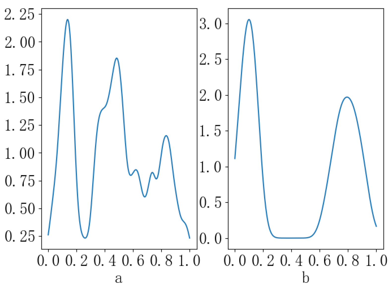
The projection of data sets with complex shapes and scattered distribution on different dimensions is different. The projection of data set 1 in Figure 1 on two dimensions is (a) and (b) in Figure 2. The more dispersed the data is in (a) dimension, the more likely it is to show the true distribution of the data; the more concentrated the data is, the more serious the overlap is. First, calculate the discreteness of each dimension. To compare the discreteness, first normalize the data by linear function. The normalization formula is (4), and the dispersion degree is calculated by Formula (5).
x = x m i n m a x m i n
Definition 2.
Discreteness. Discreteness is the degree of dispersion of the data. X = { x 1 , x 2 , x 3 , , x n } , n is the number of samples, then the discreteness of data samples is defined as:
F = i = 1 n 1 | x i + 1 x i |
According to the definition, when the point distribution is more dispersed, because the distance between all points is relatively smaller, the Discreteness value is smaller. In other words, the smaller the value of the Discreteness, the more dispersed the data. In the larger dispersed dimension, Gaussian kernel density estimation is carried out on the projection of data by using Formulas (1) and (2). Since the Gaussian kernel function is used for density probability estimation, the density function is composed of multiple normal distributions, as shown in Figure 2a.
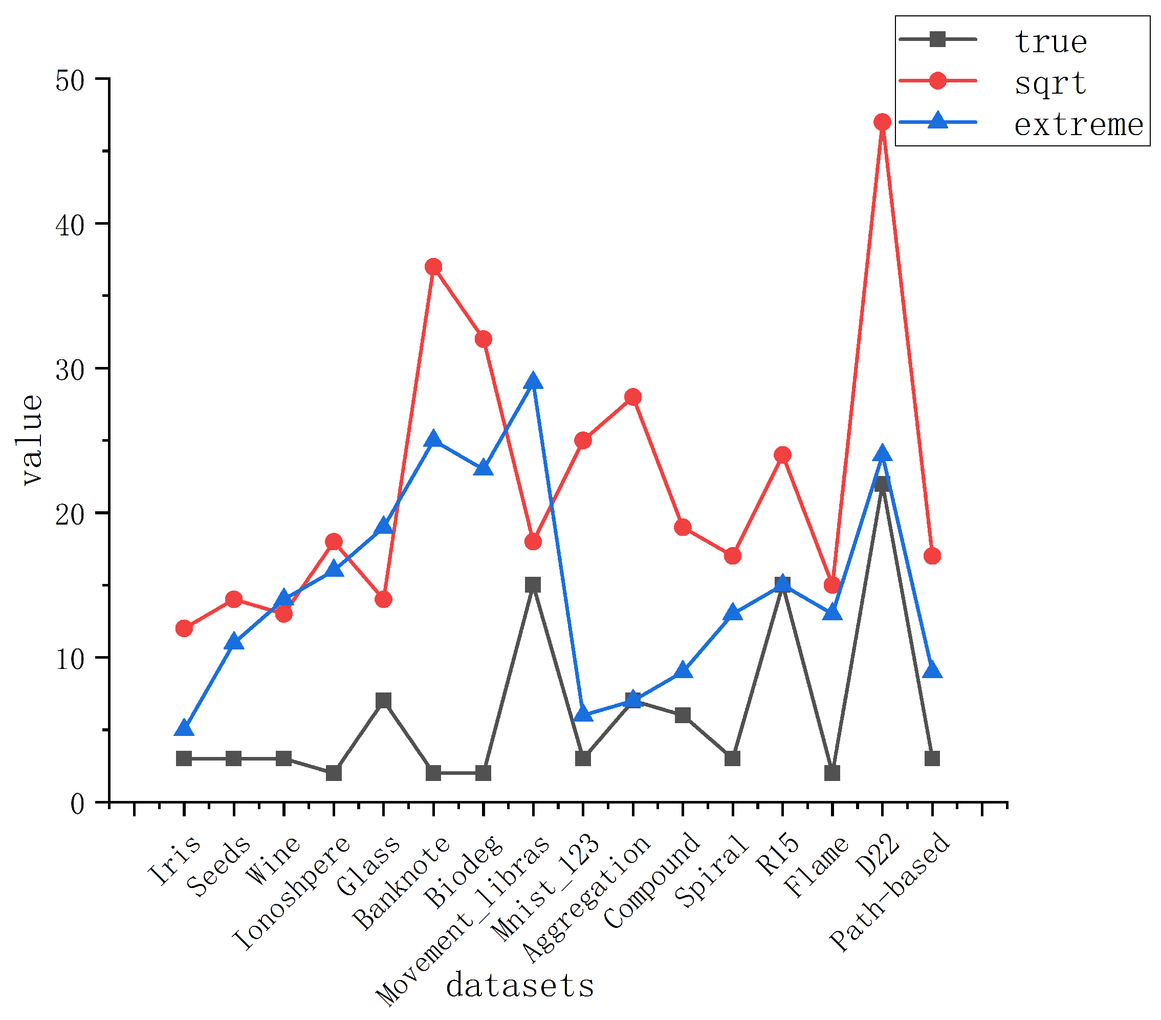
In the existing algorithms of determining the number of clusters, researchers generally directly set K m a x = n . As you can see from Figure 3, n is much larger than the actual number of clusters. At the same time, it can also be seen that the number of extreme values obtained by using gaussian kernel density function is generally smaller than the square root of n and greater than or equal to the actual number of clusters. However, occasionally, the number of extreme values is larger than n . Therefore, we will choose a small value among n and the number of extreme values as K m a x . This is also one of the reasons why the runtime performance of this algorithm is improved.

4.2. Calculation of Candidate Set of Center Points

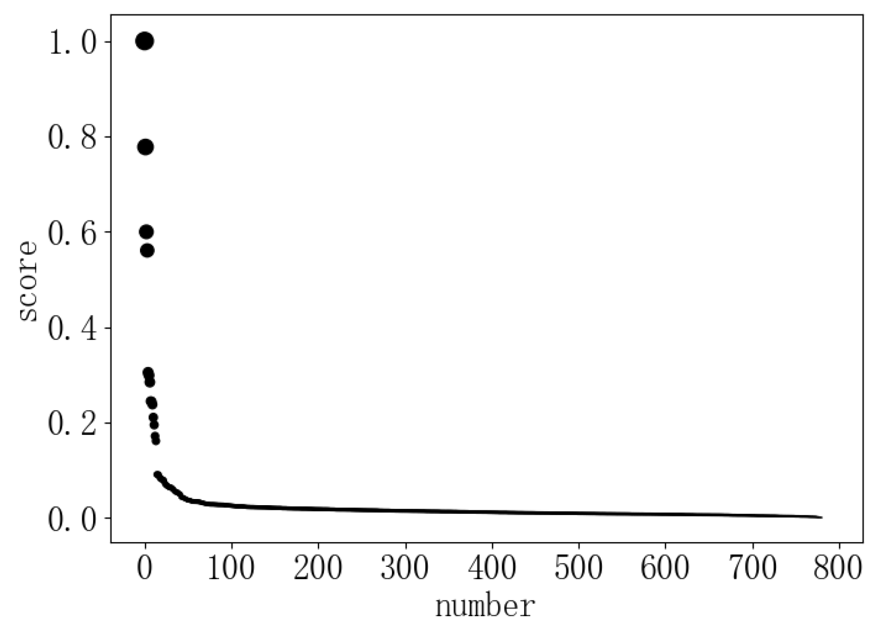
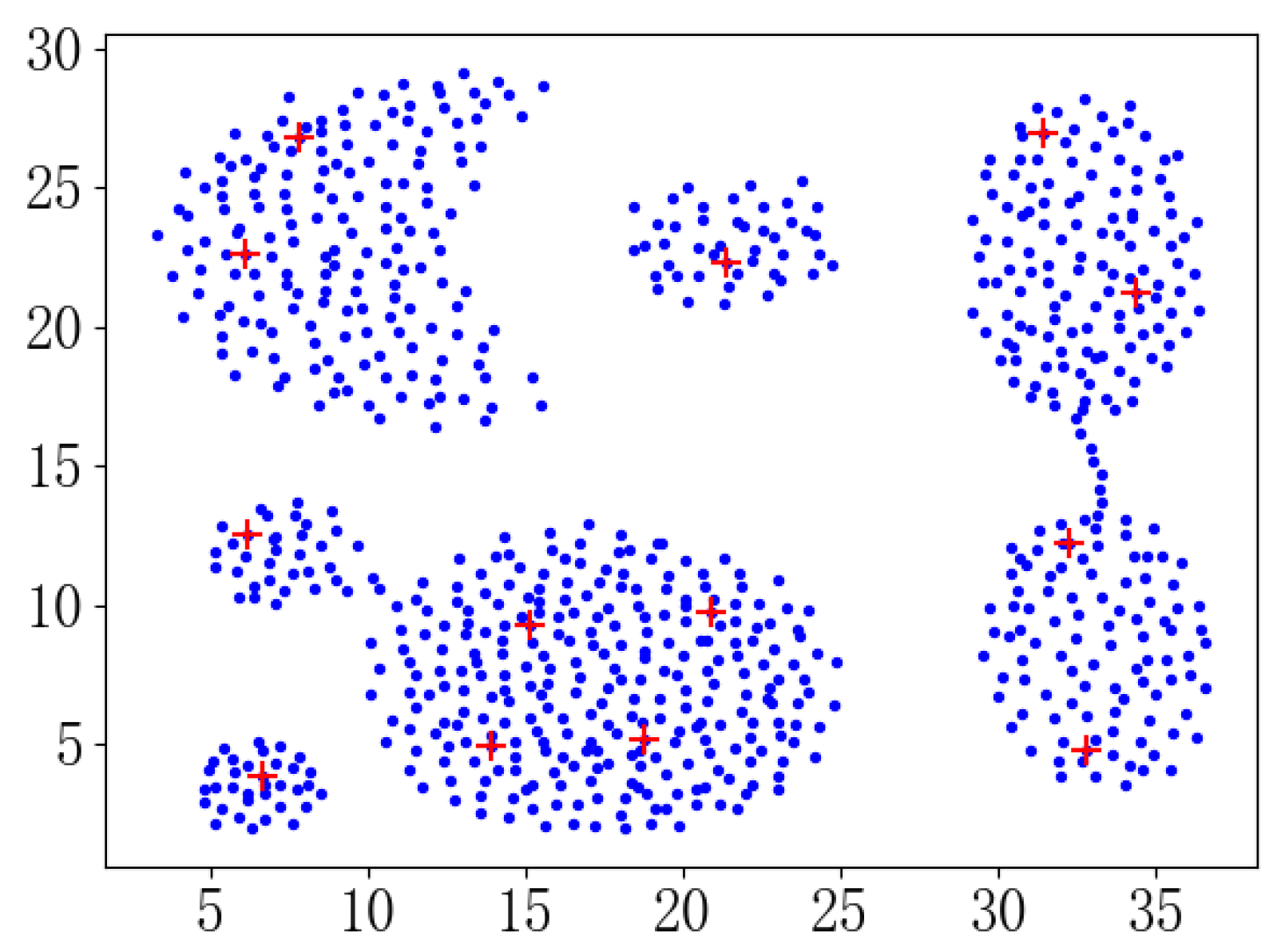
Laio et al. proposed a DPC [4] algorithm based on density peaks. The algorithm first calculates the density of each point and the minimum distance from a point that is denser than it. The algorithm visualizes the density and distance. People select the points with large density and large distance as the cluster center according to the visualization, and get the number of clusters. It requires human intervention, so it is not automated to determine the number of clusters. In general, when implementing this algorithm, the product of density and distance is often used as a score to select the center point. When the score is sorted in descending order, the K value is obtained by observing the last major change in the score. Since the change in the minimum distance between the center points is not considered, the distance between the center points may be too close. In addition, when people observe the K value, there are always some visual and subjective errors. For example, when the density parameter is optimal, the clustering effect reaches Figure 6, and the score map is shown in Figure 7. It is easy to judge that the number of clusters is 13. However, when the number of clusters is 13, as shown in Figure 8, there are already many center points in the same class.
To solve the visual error caused by manual observation and the problem of manually inputting the number of clusters, this paper proposes to use Equation (10) to automatically determine whether the score has a large change. To get the center point candidate set quickly, we use Equation (6) to calculate the score for each point and sort the scores in descending order. In Section 4.1, we obtained the maximum value K m a x of the cluster number, so we only need to judge the score change in the score of the first K m a x points. Among the points in which the score is ranked in the top K m a x , the point set consisting of points before the last significant change in the score is the center point candidate set.
s c o r e ( c i ) = m i n d e n s i t y ( c j ) > d e n s i t y ( c i ) , c i P , c j P d i s t a n c e ( c i , c j ) · d e n s i t y ( c i )
Then d e n s i t y ( c i ) is the density of point c i , d i s t a n c e ( c i , c j ) is the distance between point c i and point c j , and s c o r e ( c i ) is the score of point c i . After sorting the s c o r e ( c i ) in descending order, get G r a d e ( k ) . G r a d e ( k ) is the score ranked in the kth.
C G r a d e ( k ) = G r a d e ( k ) G r a d e ( k + 1 )
Then C G r a d e ( k ) is the score change value.
Definition 3.
Score Variation. The score variation is used to find the k value when the last great change occurred. For any 0 < k < K m a x and C G r a d e ( k ) that satisfies Formula (9), Formula (10) is calculated to calculate the score variation degree.
A v e r C G r a d e = i = 1 n 1 C G r a d e ( k ) n 1
C G r a d e ( k ) > A v e r C G r a d e
G r a d r o p ( k ) = C G r a d e ( k ) max k < i < K m a x C G r a d e ( i )
Then AverCGrade is the average of the top K m a x score changes, and G r a d r o p ( k ) is the score change degree. When G r a d r o p ( k ) a , a 2 , we think that the center point has changed greatly. For the convenience of calculation, we choose a = 2 as the condition for judging the change. Since the score does not take into account the change in the minimum distance between the center points, there may be two center points that are relatively close in the center point candidate set obtained by the change in the score. Therefore, we also need to enter Section 4.3 to judge the change of the minimum distance between the central points to avoid the two points in the same cluster.

4.3. Calculation of K Values

It can be seen from Equation (6) that the calculation of the score is calculated by assigning the same weight to the density and distance. Therefore, it is judged only by the change of the score. In the case where the local density is large, the distance between the two selected central points is very close, and it is easy to divide the data set originally of one cluster into two clusters.
Therefore, in the center point candidate set that has been obtained, we propose to make another judgment of the change in the minimum distance between the center points. When the K value is calculated by the change of the minimum distance between the center points, since the center point candidate set is calculated in Section 4.2, the center point candidate set satisfied the condition as the center point and was sorted in descending order by score. Therefore, when we select K center points, we can directly select the top K points as the center points. Since the sequence of sorting is certain, as the value of K increases, the center point that has been previously selected does not change, so the minimum distance between the center points is monotonically decreasing. We use Equation (11) to calculate the degree of change of the minimum distance between the center points. When D i s d r o p ( C k , C k + 1 ) a , a 2 , we think that the minimum distance between the center points has changed greatly. For the convenience of calculation, we make a = 2 .
D i s d r o p ( C k , C k + 1 ) = m i n c i C k , c j C k   a n d   i j d i s t a n c e ( c i , c j ) m i n c i C k + 1 , c j C k + 1   a n d   i j d i s t a n c e ( c i , c j )
When the minimum distance between center points changes greatly for the last time, when the center point is selected, the minimum distance of the center point is almost no longer changed. This shows that there is already a small distance between the two center points. In other words, the center point at this time is selected in the cluster of the existing center point. Therefore, the points before the last large change in the minimum distance between the center points are the center point set. The size of the center point set is the value of K.

4.4. Framework for Cluster Number Estimation

Step 1.
Calculate the discreteness of each dimension and find the one dimension with the largest discreteness.
Step 2.
Gaussian kernel density estimation was carried out for the one-dimensional dimension with the largest dispersion degree, and the number of extremum was obtained as Kmax.
Step 3.
Calculate the score of each point, look for the point with the last great change among the points with the score in the first K m a x , and get the candidate set, whose size is denoted as K m a x .
Step 4.
Calculate the minimum distance between the center points when the K value is from 1 to K m a x . The points before the last large change in the minimum distance between the center points are the center point set, and the size of the center point set is calculated to obtain the K value;

5. Experiments and Discussion

5.1. Experimental Environment, Dataset and Other Algorithms

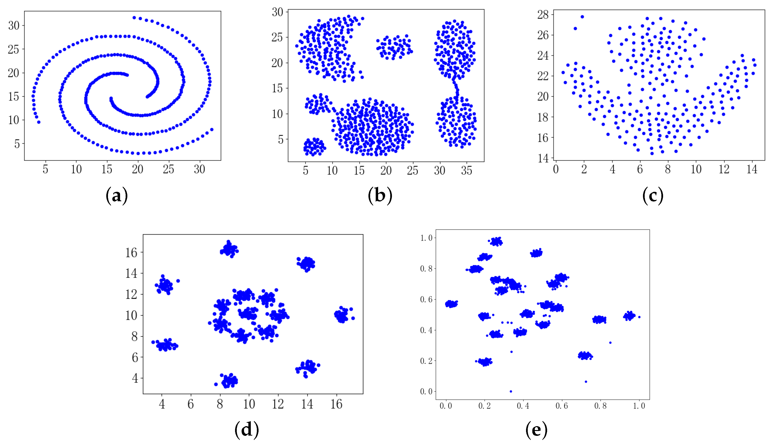
In this paper, 8 UCI real datasets, a subset of MNIST (The MNIST is a set of handwritten digits) and 5 artificial datasets (Sprial, Aggregation, Flame, R15, D22) are used to verify the effectiveness of the proposed algorithm, and 11 algorithms such as BIC, CH and PC are compared with our approach. Where Mnist_123 is a subset of the MNIST and contains handwritten digits “1”, “2”, and “3”.
The experimental simulation environment is Pycharm2019, the hardware configuration is Intel(R)Core(TM) i5-2400m CPU @3.1ghz, 4GB memory, 270G hard disk, and the operating system is Windows 10 professional version.
The shape structures of the five artificial datasets are illustrated in Figure 9. The detailed information of the seven data sets is shown in Table 2.
In the analysis and comparison of the results, we evaluates the algorithm in this paper and other 11 algorithms from the aspects of the accuracy of the number of clusters and time performance of estimation. The detailed information of these 11 algorithms is shown in Table 3. The accuracy of each algorithm is obtained by analyzing the results of 20 runs of each data. The time performance of each algorithm is evaluated by the average time obtained by running each data 20 times.

5.2. Experimental Results and Analysis

The results of the algorithm in this paper and the other 11 algorithms running 20 times on 14 data sets are shown in Table 4. For an algorithm performing 20 times on a data set, two results are separated by “/”, and multiple results are separated by “-”.
Table 4 shows the results of each algorithm when estimating the number of clusters on different data sets. Figure 10 shows the correct number of cluster estimates for each algorithm on 14 data sets. As can be seen from Table 4 and Figure 9, the BIC and LL algorithms can correctly estimate the number of clusters of the two data sets. The effects of PBMF and LML are slightly better than them, and the number of clusters can be correctly estimated on three data sets. The CE and I index algorithms also show higher accuracy, which can correctly estimate the number of clusters of 4 data sets, while the CH, Jump, and PC algorithms have higher accuracy, and can correctly estimate the number of clusters of 6 data sets. However, these algorithms are generally not ideal for estimating the datasets such as Wine, Glass, Aggregation, Movement_libras, and Mnist_123. The algorithm of this paper can correctly determine the number of clusters of these 14 data sets, and the correct rate is the highest.
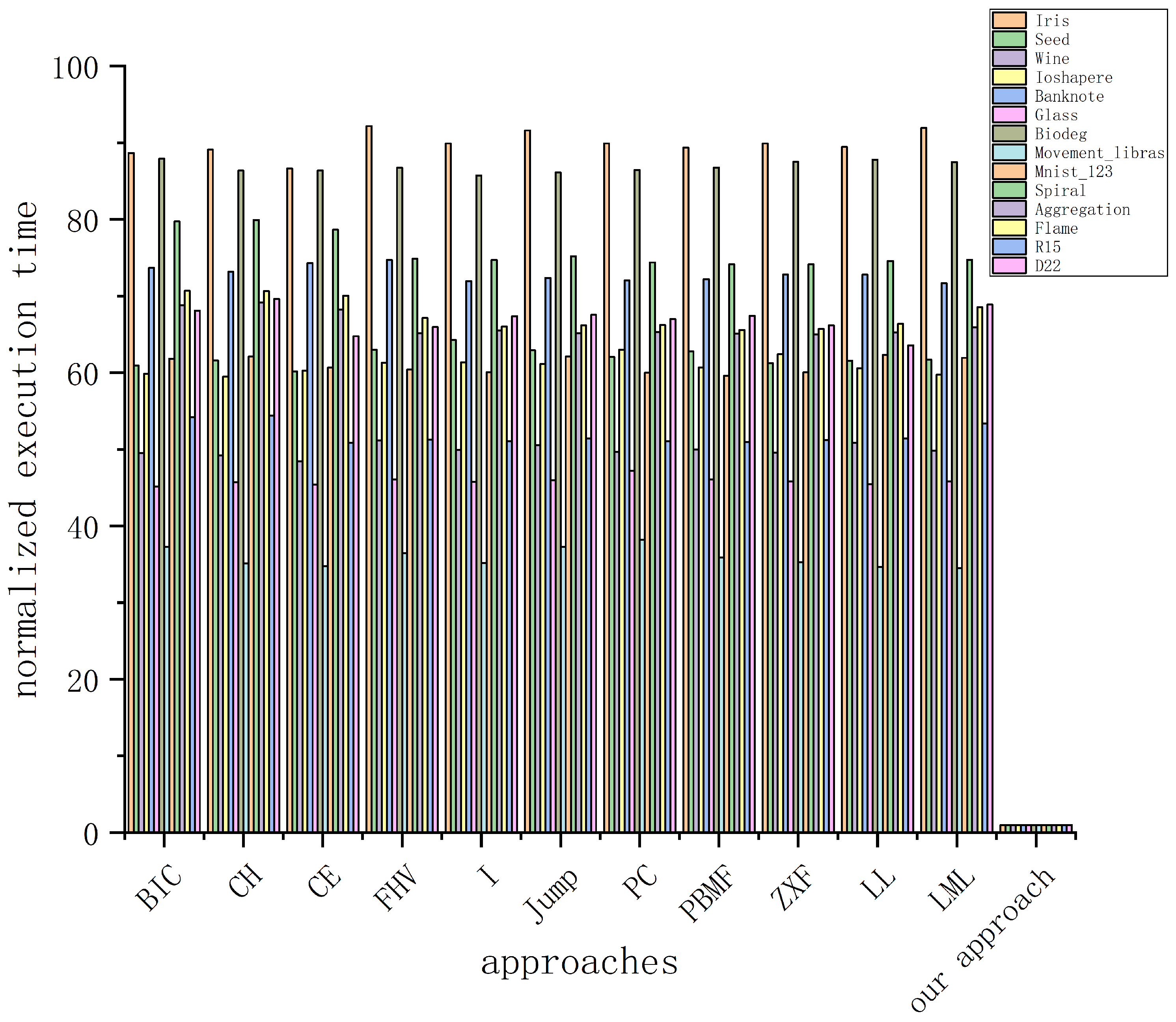
Beside accuracy, time performance is also compared in this paper. In this paper, the average time for each algorithm to execute 20 times on each data set is taken as the running time, and the results are shown in Table 5. It can be seen that the running time of the remaining 11 algorithms on Iris is more than 1.3, while the running time of the algorithm in this paper is 0.015. Moreover, the running time of other algorithms on other data sets is about 50 times of the running time of this algorithm. The running time on some data sets is even nearly a hundred times. Therefore, you can see the improvement in time performance of this algorithm.
Figure 11 shows normalized execution time of each of the approaches. The normalized execution time of an approach on a data set is obtained by dividing the execution time of that approach by that of our approach on the same data set. According to the figure, the performance of our method is much higher than other methods. All other solutions show similar performance on the same data set.
Our improvement in time performance is closely related to the selection of K m a x and center point. Other algorithms directly set K m a x = n , while the algorithm in this paper obtained K m a x value through one-dimensional Gaussian Kernel density, which greatly reduced the range of K m a x and saved time. When selecting the center point, the algorithm in this paper calculates the score at one time and selects the first K points according to different K values. Because the other 11 algorithms need not only the center point, but also the clustering results. Therefore, clustering should be conducted according to different K values each time to obtain the score of each index. The clustering process needs multiple iterations, which is also one of the reasons why they consume huge time.

6. Conclusions

This paper mainly deals with the estimation of cluster number of data sets with complex and scattered shape. To improve the accuracy of the cluster number estimation and improve the time performance of the estimation, we use the Gaussian Kernel function to obtain the K m a x value to narrow the judgment range, and use the change of the center point score and the change of the minimum distance between the center points to obtain the K value. Experimental results show that the proposed algorithm is practical and effective. Since the optimal density parameters of the algorithm are not yet automatically determined, we will further study how to automatically determine the optimal density parameters.

Author Contributions

Methodology, Z.H.; Validation, Z.H.; Formal Analysis, Z.J. and X.Z.; Writing—Original Draft Preparation, Z.H.; Resources, Z.H.; Writing—Review & Editing, Z.J. and X.Z.; Visualization, Z.H.; Supervision, Z.J.; Project Administration, Z.J.; Funding Acquisition, Z.J. All authors have read and agreed to the published version of the manuscript.

Funding

This research received no external funding.

Acknowledgments

The authors are very grateful to Henan Polytechnic University for providing the authors with experimental equipment. At the same time, the authors are grateful to the reviewers and editors for their suggestions for improving this article.

Conflicts of Interest

The authors declare no conflict of interest.

References

  1. Jain, A.K. Data clustering: 50 years beyond K-means. Pattern Recognit. Lett. 2010, 31, 651–666. [Google Scholar] [CrossRef]
  2. Ren, M.; Liu, P.; Wang, Z.; Yi, J. A self-adaptive fuzzy c-means algorithm for determining the optimal number of clusters. Comput. Intell. Neurosci. 2016, 2016, 2647389. [Google Scholar] [CrossRef] [Green Version]
  3. Zhou, X.; Miao, F.; Ma, H. Genetic algorithm with an improved initial population technique for automatic clustering of low-dimensional data. Information 2018, 9, 101. [Google Scholar] [CrossRef] [Green Version]
  4. Rodriguez, A.; Laio, A. Machine learning Clustering by fast search and find of density peaks. Science 2014, 344, 1492. [Google Scholar] [CrossRef] [Green Version]
  5. Yang, X.H.; Zhu, Q.P.; Huang, Y.J.; Xiao, J.; Wang, L.; Tong, F.C. Parameter-free Laplacian centrality peaks clustering. Pattern Recognit. Lett. 2017, 100, 167–173. [Google Scholar] [CrossRef]
  6. Fujita, A.; Takahashi, D.Y.; Patriota, A.G. A non-parametric method to estimate the number of clusters. Comput. Stat. Data Anal. 2014, 73, 27–39. [Google Scholar] [CrossRef]
  7. Maulik, U.; Bandyopadhyay, S. Performance evaluation of some clustering algorithms and validity indices. IEEE Trans. Pattern Anal. Mach. Intell. 2002, 24, 1650–1654. [Google Scholar] [CrossRef] [Green Version]
  8. Xie, X.L.; Beni, G. A validity measure for fuzzy clustering. IEEE Trans. Pattern Anal. Mach. Intell. 1991, 8, 841–847. [Google Scholar] [CrossRef]
  9. Davies, D.L.; Bouldin, D.W. A cluster separation measure. IEEE Trans. Pattern Anal. Mach. Intell. 1979, 2, 224–227. [Google Scholar] [CrossRef]
  10. Teklehaymanot, F.K.; Muma, M.; Zoubir, A.M. A Novel Bayesian Cluster Enumeration Criterion for Unsupervised Learning. IEEE Trans. Signal Process. 2017, 66, 5392–5406. [Google Scholar] [CrossRef] [Green Version]
  11. Masud, M.A.; Huang, J.Z.; Wei, C.; Wang, J.; Khan, I.; Zhong, M. I-nice: A new approach for identifying the number of clusters and initial cluster centres. Inf. Sci. 2018, 466, 129–151. [Google Scholar] [CrossRef]
  12. Wang, Y.; Shi, Z.; Guo, X.; Liu, X.; Zhu, E.; Yin, J. Deep embedding for determining the number of clusters. In Proceedings of the Thirty-Second AAAI Conference on Artificial Intelligence, New Orleans, LA, USA, 2–7 February 2018. [Google Scholar]
  13. Kingrani, S.K.; Levene, M.; Zhang, D. Estimating the number of clusters using diversity. Artif. Intell. Res. 2018, 7, 15–22. [Google Scholar] [CrossRef] [Green Version]
  14. Zhou, S.; Xu, Z. A novel internal validity index based on the cluster centre and the nearest neighbour cluster. Appl. Soft Comput. 2018, 71, 78–88. [Google Scholar] [CrossRef]
  15. Li, X.; Liang, W.; Zhang, X.; Qing, S.; Chang, P.C. A cluster validity evaluation method for dynamically determining the near-optimal number of clusters. Soft Comput. 2019. [Google Scholar] [CrossRef]
  16. Ünlü, R.; Xanthopoulos, P. Estimating the number of clusters in a dataset via consensus clustering. Expert Syst. Appl. 2019, 125, 33–39. [Google Scholar] [CrossRef]
  17. Khan, I.; Luo, Z.; Huang, J.Z.; Shahzad, W. Variable weighting in fuzzy k-means clustering to determine the number of clusters. IEEE Trans. Knowl. Data Eng. 2019. [Google Scholar] [CrossRef]
  18. Sugar, C.A.; James, G.M. Finding the number of clusters in a dataset: An information-theoretic approach. J. Am. Stat. Assoc. 2003, 98, 750–763. [Google Scholar] [CrossRef]
  19. Tong, Q.; Li, X.; Yuan, B. A highly scalable clustering scheme using boundary information. Pattern Recognit. Lett. 2017, 89, 1–7. [Google Scholar] [CrossRef]
  20. Zhou, S.; Xu, Z.; Liu, F. Method for determining the optimal number of clusters based on agglomerative hierarchical clustering. IEEE Trans. Neural Netw. Learn. Syst. 2016, 28, 3007–3017. [Google Scholar] [CrossRef]
  21. Gupta, A.; Datta, S.; Das, S. Fast automatic estimation of the number of clusters from the minimum inter-center distance for k-means clustering. Pattern Recognit. Lett. 2018, 116, 72–79. [Google Scholar] [CrossRef]
  22. Silverman, B.W. Density Estimation for Statistics and Data Analysis; Chapman and Hall: London, UK, 1986. [Google Scholar]
  23. Caliński, T.; Harabasz, J. A dendrite method for cluster analysis. Commun. Stat.-Theory Methods 1974, 3, 1–27. [Google Scholar] [CrossRef]
  24. Bezdek, J.C. Mathematical models for systematics and taxonomy. In Proceedings of the 8th International Conference on Numerical; Freeman: San Francisco, CA, USA, 1975; Volume 3, pp. 143–166. [Google Scholar]
  25. Dave, R.N. Validating fuzzy partitions obtained through c-shells clustering. Pattern Recognit. Lett. 1996, 17, 613–623. [Google Scholar] [CrossRef]
  26. Bezdek, J.C. Cluster validity with fuzzy sets. J. Cybernet. 1973, 3, 58–73. [Google Scholar] [CrossRef]
  27. Pakhira, M.K.; Bandyopadhyay, S.; Maulik, U. Validity index for crisp and fuzzy clusters. Pattern Recognit. 2004, 37, 487–501. [Google Scholar] [CrossRef]
  28. Zhao, Q.; Xu, M.; Fränti, P. Sum-of-squares based cluster validity index and significance analysis. In International Conference on Adaptive and Natural Computing Algorithms; Springer: Berlin/Heidelberg, Germany, 2009; pp. 313–322. [Google Scholar]
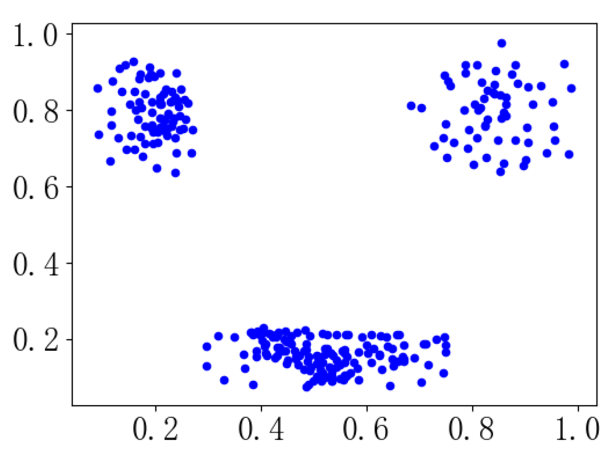
Figure 1. Shape structure of dataset 1.
Information 11 00016 g001
Figure 2. Gaussian kernel distribution on each dimension. (a) Gaussian kernel distribution in X dimension; (b) Gaussian kernel distribution in Y dimension.
Information 11 00016 g002
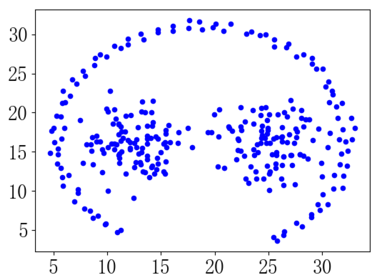
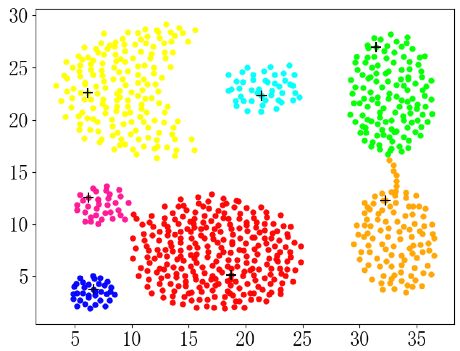
Figure 3. Comparison between the number of extreme values and the real k value and n . (Here, “true” represents the true cluster number of the data set, “sqrt” represents the square root of the size of the data set, and “extreme” represents the extreme number of density estimated by gaussian kernel density. The data shape of Compound is shown in Figure 4. It consists of 399 points and two attributes, which are divided into six clusters. The path-based graphic shape is shown in Figure 5. It consists of 300 points and two attributes, which are divided into three clusters. Details of the other data sets are described in Section 5).
Information 11 00016 g003
Figure 4. Shape structure of compound dataset.
Information 11 00016 g004
Figure 5. Shape structure of path-based dataset.
Information 11 00016 g005
Figure 6. The correct clustering result of the aggregation data set.
Information 11 00016 g006
Figure 7. Score graph of aggregation dataset.
Information 11 00016 g007
Figure 8. Center point distribution when the number of clusters is 13.
Information 11 00016 g008
Figure 9. Datasets of different shape structures. (a) Spiral, (b) Aggregation, (c) Flame, (d) R15, (e) D22.
Information 11 00016 g009
Figure 10. The correct number of each algorithm.
Information 11 00016 g010
Figure 11. Normalized execution time comparison.
Information 11 00016 g011
Table 1. Notions.
Table 1. Notions.
NotionsDescription
Pnode set
minthe minimum value of a set of values
maxthe maximum value of a set of values
K m a x maximum number of clusters
K m a x the size of the candidate point set
Knumber of clusters
Fthe value of Discreteness
C K center point set with the number of center points being K
c i point i
G r a d e ( k ) the score of the kth point in descending order
G r a d r o p ( k ) the change of the kth point in score
A v e r C G r a d e average of the top Kmax score changes
d i s t a n c e ( C i , C j ) Euclidean distance between point i and point j
D i s d r o p ( C k , C k + 1 ) the degree of change of the minimum distance when the number of center points is from k to k + 1
Table 2. Details of dataset.
NumberDatasetFeaturesClustersInstances
1Iris43150
2Seeds73210
3Wine133178
4Ionoshpere342351
5Banknote421372
6Glass97214
7Biodeg4121055
8Movement_libras9115366
9Mnist_1237843649
10Spiral23312
11Aggregation27788
12Flame22240
13R15215600
14D222222211
Table 3. Approaches to be compared with ours.
NumberApproachesSelection Criteria for KMin No. of Clusters
1Bayesian Information Criterion (BIC)max2
2Caliński Harabasz (CH) Index [23]max2
3Classification Entropy (CE) [24]min2
4Fuzzy Hypervolume (FHV) [25]min1
5I Index [7]max2
6Jump Method [18]max2
7Partition Coefficient (PC) [26]max2
8PBMF [27]max2
9Zhao Xu Fränti (ZXF) Index [28]Knee2
10Last leap (LL) [21]max & 11
11Last Major Leap (LML) [21]max & 11
12our approachmax & 11
Table 4. Estimation of the optimal number of clusters in overlapping data sets.
ApproachesIrisSeedsWineIonoshpereBanknoteGlassBiodegMovement_librasMnist_123SpiralAggregationFlameR15D22
BIC8–12141315–1835–371431/321823–2531441525–33
CH3313221422215–1726–2881523–25
CE22222222222222
FHV21111411111111
I337234–64222441523
Jump3310–13215–371322212–1714–2741522
PC2222222222221522
PBMF3312/13315–3713/144/53/427/8441523
ZXF6664–7964/55-105-85/664811
LL2221–11221–3121/241641523–26
LML3221–9221/62–1711641524–26
our approach33322721533721522
Table 5. Execution time of approaches.
ApproachesIrisSeedWineIoshapereBanknoteGlassBiodegMovement_librasMnist_123SpiralAggregationFlameR15D22
BIC1.3482.0171.5703.96224.0232.13420.8214.02537.3403.53310.1502.4115.72042.149
CH1.3542.0391.5603.93823.8632.16320.4513.79437.5053.54110.2032.4095.74043.090
CE1.3171.9911.5343.99024.2292.14820.4553.75736.6363.48410.0612.3895.36740.092
FHV1.4012.0851.6224.05924.3592.17920.5413.93936.4793.3179.6122.2905.40940.817
I1.3672.1271.5834.06023.4582.16620.2993.79736.2613.3089.6592.2515.38641.698
Jump1.3932.0831.6034.04823.6032.17520.3914.02537.5043.3329.6052.2575.42741.829
PC1.3672.0541.5764.17123.4932.23320.4714.12536.2313.2959.6312.2585.39041.474
PBMF1.3592.0781.5854.01723.5422.17820.5483.87936.0093.2859.6022.2365.37841.730
ZXF1.3672.0281.5724.13123.7342.16720.7183.81036.2603.2839.5922.2415.40340.958
LL1.3602.0381.6134.00823.7372.15120.7893.74437.6253.3049.6242.2635.42339.356
LML1.3972.0431.5803.95423.3702.16720.7113.72737.4063.3119.7222.3375.62942.636
our approach0.0150.0330.0320.0660.3260.0470.2370.1080.6040.0440.1480.0340.1060.619