1. Introduction
The observation, monitoring, and estimation of rainfall are matters of major concern for a number of reasons. For instance, public administrators aim at guaranteeing an adequate level of security for people living and operating on a given territory: for this purpose, rainfall forecasting is key for the assessment of hydrogeological risks due to landslides and floods. An accurate measurement of total rainfall amount is also critical in climatological studies, since it represents one of the main climate indices. Moreover, the knowledge of the real-time rain rate during precipitation events is useful in urban areas to estimate water runoff from the drainage system.
A very high spatial and temporal variability characterizes rainfall [
1,
2,
3]: it is then difficult to obtain accurate measurements with proper spatial density and temporal detail. Several instruments and techniques have been developed to gauge this quantity (e.g., the use of weather radars, rain gauges, infrared satellite imagery, microwave links, etc.). Each of them presents advantages and limitations [
4]: for example, remote sensing measurements aim at estimating the precipitation field over wide areas, but typically with limited spatial resolution and accuracy; on the contrary, point observations, e.g., collected by rain gauges and disdrometers, deliver precise local measurements, but they hardly provide large and dense coverage.
Recently, increasing attention has been paid to the exploitation of satellite downlink signals for the estimation of rainfall, as most of the commercial satellite communication systems currently operate in the Ku band (12–18 GHz) and the K band (18–26 GHz): in fact, in such a frequency range, rain significantly impairs the propagation of electromagnetic waves [
5,
6]. Some approaches have been developed for estimating the intensity of precipitation on a large scale from space-borne signals, with a spatiotemporal resolution between that of rain gauges and of weather radars. In fact, the opportunistic use of satellite downlink signals to estimate rainfall combines the benefit of covering areas where ground instrumentation or radar networks are not available, and the requirement of high temporal resolution measurements, which is in the order of one minute [
7]: this approach would allow providing two-dimensional maps of the rain intensity, even across continental regions (e.g., Europe) by using a sufficiently dense network of ground receivers.
The methodologies that are currently available to assess rainfall rate via satellite links are of limited accuracy and reliability and, in some cases, of complex implementation [
8,
9,
10,
11]: as a consequence, it becomes necessary to investigate alternative estimation methods, which only require few measurable physical parameters as input.
This contribution presents a novel estimation methodology that aims to estimate the rain rate by opportunistically exploiting local downlink satellite communication signals and by making use of local ancillary meteorological data, namely the hourly zero-degree isotherm height and the monthly convectivity index. The model also includes different expressions to take the different impact of stratiform and convective rain events on the link into due account. More specifically, the remainder of the paper is structured as follows.
Section 2 presents the Earth-space propagation experiment carried out at Politecnico di Milano, along with the experimental setup used in this work.
Section 3 describes the experimental datasets.
Section 4 describes the proposed prediction methodology in detail, while
Section 5 summarizes the full procedure for rain rate estimation. Lastly,
Section 6 discusses the performance of the proposed model (as well as of other methodologies that are available in the literature) and
Section 7 draws some conclusions.
6. Performance Evaluation
The calibration of the model’s parameters was carried out on a statistical basis, i.e., by maximizing the agreement between the measured and estimated However, it is worth verifying the accuracy in estimating the rain rate applicability when the model is used on an instantaneous basis. To this aim, we have resorted to the following indicators of the rain event:
total rainfall accumulation, [mm];
maximum rain rate, [mm/h]; and,
average rain rate, [mm/h].
For each indicator, we have defined the difference between the daily estimated (denoted with the subscript
) and measured (denoted with the subscript
) quantity of interest, for each of the 70 considered rain events:
Table 5 lists the associated average (on all the events) mean and RMS values of the residuals.
The results obtained are satisfactory, as the indicators reveal that the proposed method allows (on average) for estimating the rainfall accumulation with an error in the order of few millimeters. Concerning the detection of peak rain rates, the resulting value of the RMS error is considered to be acceptable, given the difficulty in estimating extreme rain rate values, which might even range between 150 mm/h and 200 mm/h.
Besides the overall statistical indicators, it is worth further investigating the model accuracy by selecting some sample events.
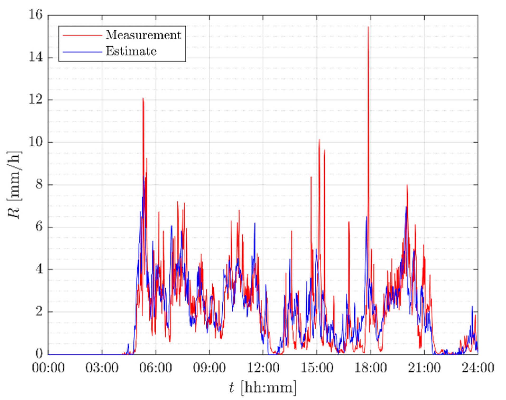
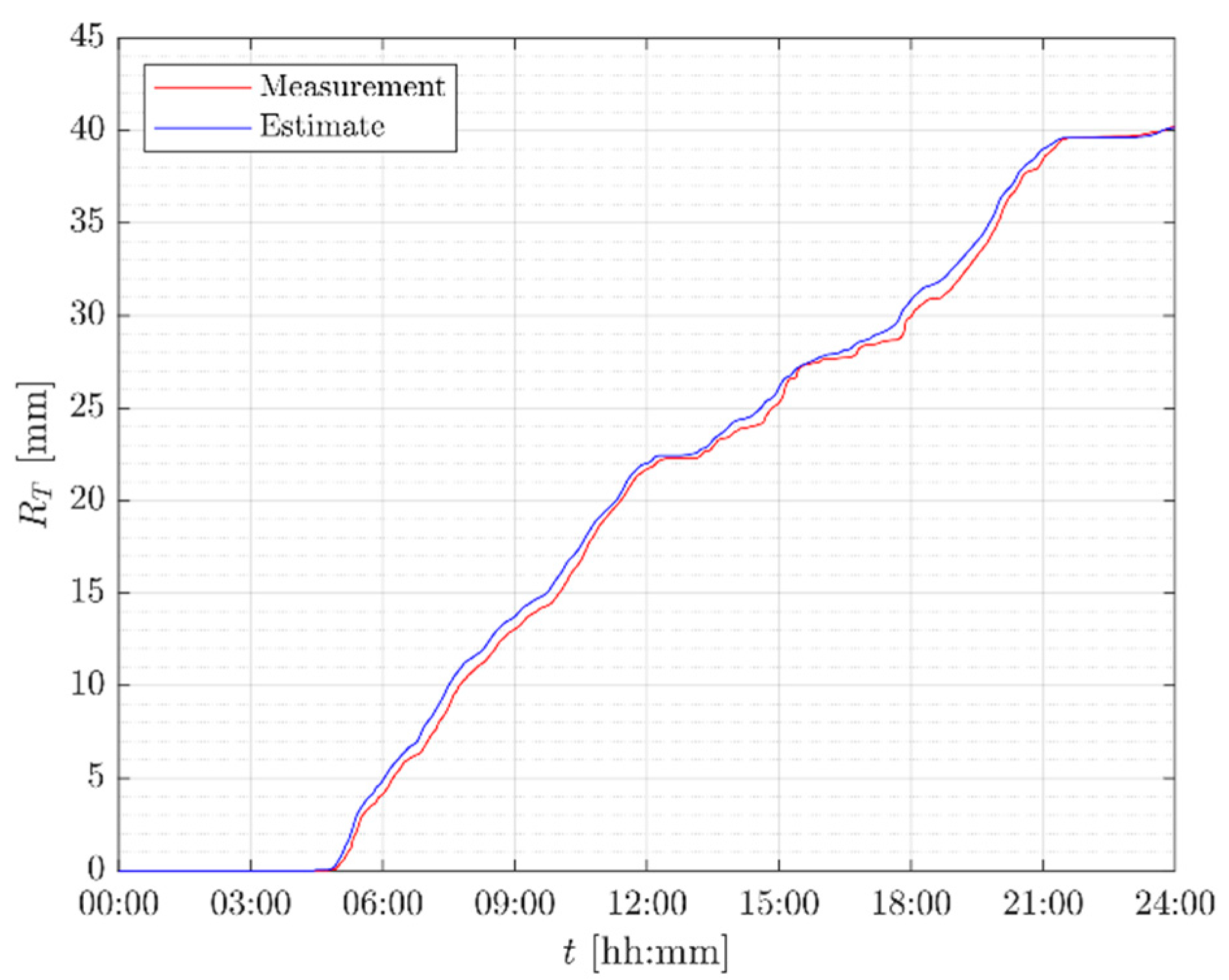
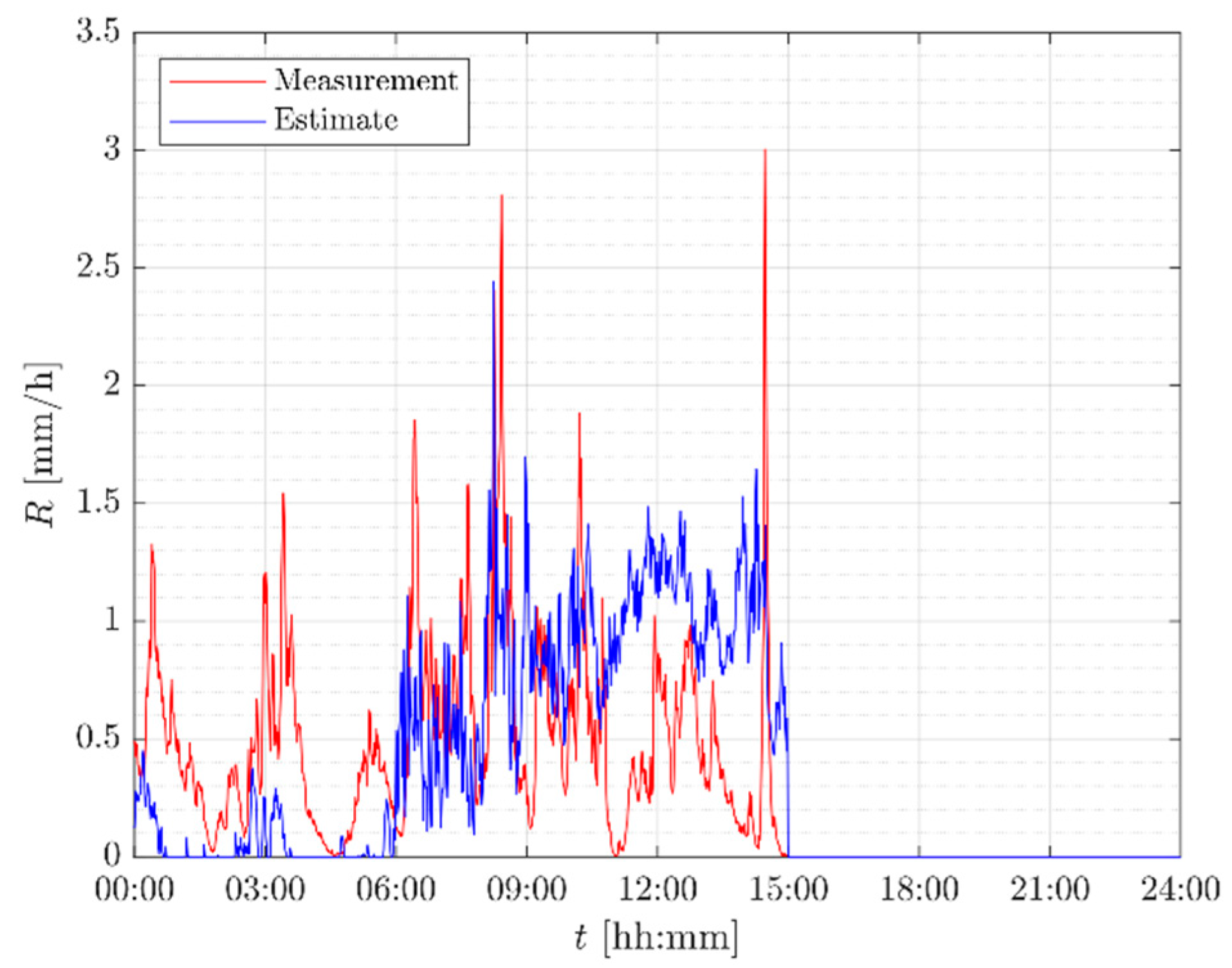
Figure 11 depicts the trend of the rain rate during a typical Spring rain event, which is characterized by moderate rain rates and occasional more intense peaks. The equivalent rain height is calculated while using (10) since the event occurred in April (
: the variability of the precipitation is tracked with a significant degree of accuracy, leading to an estimate of the total rainfall accumulation that closely matches the measurements (see
Figure 12).
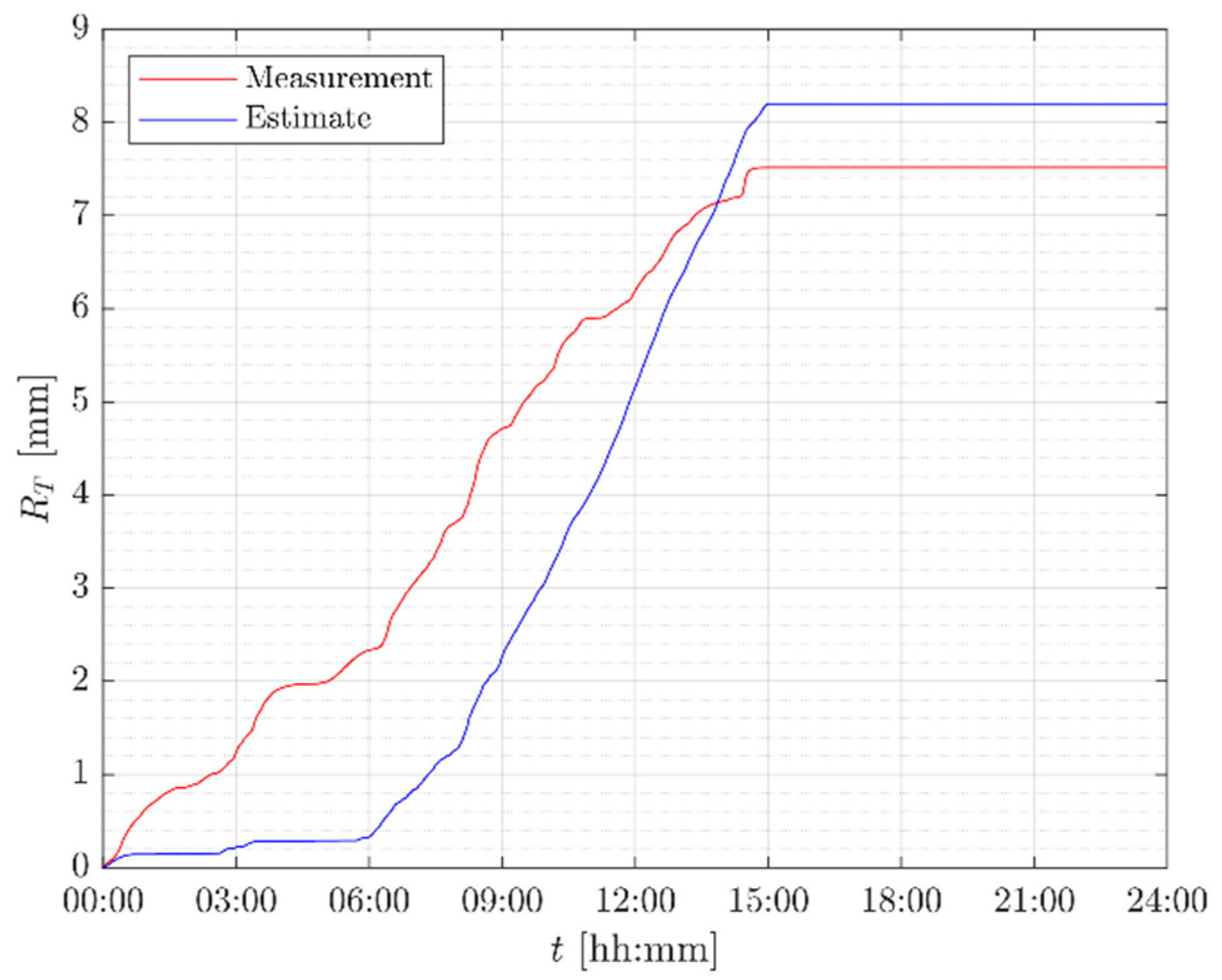
Figure 13 and
Figure 14 refer to a typical event in Autumn (November,
): in this case, the equivalent rain height is calculated while using (8). The model accuracy is lower than in the previous event, but the results are still quite satisfactory.
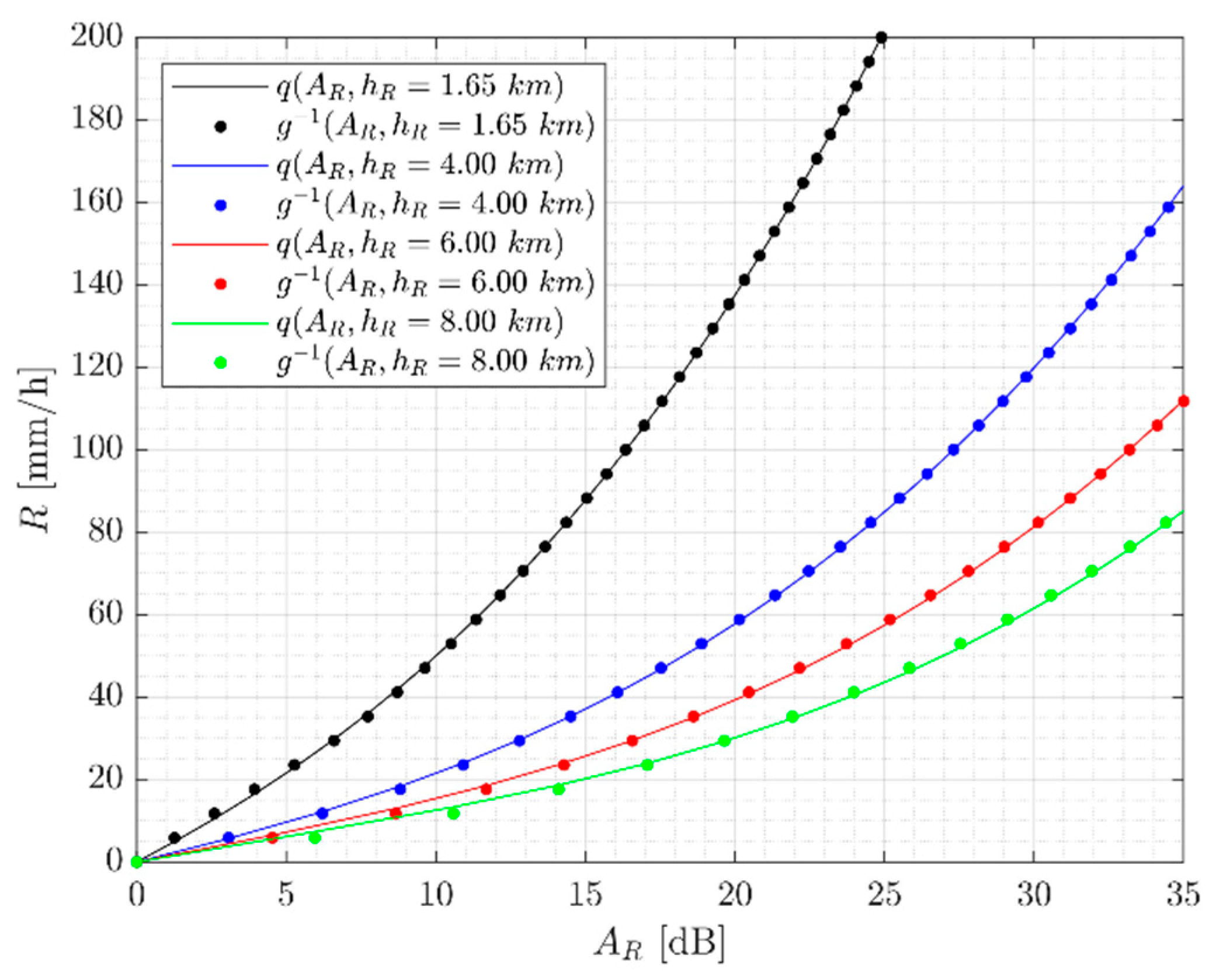
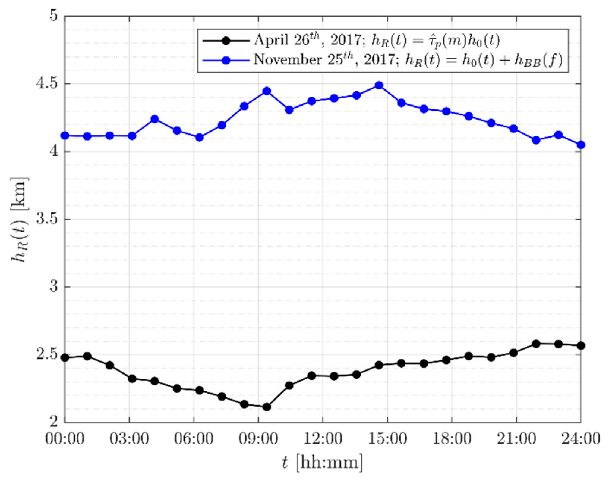
The correct evaluation of the equivalent rain height plays a key role in the prediction of the rain rate, as also shown by the curves in
Figure 7.
Figure 15 depicts the trend of
for the previously mentioned convective and stratiform events, as reported in
Figure 11 and
Figure 13, respectively, and points out the importance of using local forecast values of
with high temporal resolution. The values in
Figure 15 indicate the opposite for the two events, although the rain height is generally higher for convective events than for stratiform ones; in this case, using monthly values of
(or even worst, a single yearly value) would have led to a much lower prediction accuracy than that shown in
Figure 11 and
Figure 13.
Author Contributions
Conceptualization, L.L. and C.G.R.; methodology, R.A.G., L.L. and C.G.R.; software, R.A.G., L.L. and C.G.R.; validation, R.A.G. and L.L.; formal analysis, R.A.G. and L.L.; investigation, L.L. and C.G.R.; writing—original draft preparation, R.A.G.; writing—review and editing, R.A.G., L.L. and C.G.R.; visualization, R.A.G.; supervision, L.L. and C.G.R.; project administration, L.L. and C.G.R. All authors have read and agreed to the published version of the manuscript.
Funding
This work was partially supported by the Air Force Office of Scientific Research, Air Force Material Command, United States Air Force, European Office of Aerospace Research and Development under Grant FA9550-17-1-0335.
Acknowledgments
The Authors want to thank NASA for making the propagation data available.
Conflicts of Interest
The authors declare no conflict of interest. The funders had no role in the design of the study; in the collection, analyses, or interpretation of data; in the writing of the manuscript, or in the decision to publish the results.
References
- Jorge, F.; Rocha, A.; Mota, S. Evaluation of inter-annual variability of rainfall rate and rain attenuation based on the ITU rec P.678. In Proceedings of the 9th European Conference on Antennas and Propagation (EuCAP), Lisbon, Portugal, 13–17 April 2015. [Google Scholar]
- Gader, K.; Gara, A.; Slimani, M.; Raouf, M.M. Study of spatio-temporal variability of the maximum daily rainfall. In Proceedings of the 2015 6th International Conference on Modeling, Simulation, and Applied Optimization (ICMSAO), Istanbul, Turkey, 27–29 May 2015; pp. 1–6. [Google Scholar]
- Pimienta-del-Valle, D.; Garcia-del-Pino, P.; Riera, J.M.; Siles, G.A. A four-year variability study for Ka- and Q-band slant path propagation experiments in Madrid. In Proceedings of the 13th European Conference on Antennas and Propagation (EuCAP), Krakow, Poland, 31 March–5 April 2019. [Google Scholar]
- Giannetti, F.; Reggiannini, R.; Moretti, M.; Adirosi, E.; Baldini, L.; Facheris, L.; Antonini, A.; Melani, S.; Bacci, G.; Petrolino, A.; et al. Real-Time Rain Rate Evaluation via Satellite Downlink Signal Attenuation Measurement. Sensors 2017, 17, 1864. [Google Scholar] [CrossRef] [PubMed]
- Crane, R.K. Electromagnetic Wave Propagation through Rain; Wiley: Hoboken, NJ, USA, 1996. [Google Scholar]
- Louis, J. Satellite Communications Systems Engineering; Wiley: Hoboken, NJ, USA, 2008. [Google Scholar]
- International Telecommunications Union. Recommendation ITU-R P.837, Characteristics of Precipitation for Propagation Modelling; International Telecommunications Union: Geneva, Switzerland, 2017. [Google Scholar]
- Gharanjik, A.; Shankar, M.R.B.; Zimmer, F.; Ottersten, B. Centralized Rainfall Estimation Using Carrier to Noise of Satellite Communication Links. IEEE J. Sel. Areas Commun. 2018, 36, 1065–1073. [Google Scholar] [CrossRef] [Green Version]
- Giannetti, F.; Moretti, M.; Reggiannini, R.; Vaccaro, A. The NEFOCAST System for Detection and Estimation of Rainfall Fields by the Opportunistic Use of Broadcast Satellite Signals. IEEE Aerosp. Electron. Syst. Mag. 2019, 34, 16–27. [Google Scholar] [CrossRef]
- Csurgai-Horvath, L.; Bito, J. Rain Intensity Estimation Using Satellite Beacon Signal Measurements a Dual Frequency Study. In Proceedings of the 2018 International Symposium on Networks, Computers and Communications (ISNCC), Rome, Italy, 19–21 June 2018; pp. 1–5. [Google Scholar]
- Adirosi, E.; Facheris, L.; Petrolino, A.; Giannetti, F.; Reggiannini, R.; Moretti, M.; Scarfone, S.; Melani, S.; Collard, F.; Bacci, G. Exploiting satellite Ka and Ku links for the real-time estimation of rain intensity. In Proceedings of the 2017 XXXIInd General Assembly and Scientific Symposium of the International Union of Radio Science (URSI GASS), Montreal, QC, Canada, 19–26 August 2017; pp. 1–4. [Google Scholar]
- Rossi, T.; De Sanctis, M.; Ruggieri, M.; Riva, C.; Luini, L.; Codispoti, G.; Russo, E.; Parca, G. Satellite communication and propagation experiments through the alphasat Q/V band Aldo Paraboni technology demonstration payload. IEEE Aerosp. Electron. Syst. Mag. 2016, 31, 18–27. [Google Scholar] [CrossRef]
- Zemba, M.; Nessel, J.; Houts, J.; Luini, L.; Riva, C. Statistical analysis of instantaneous frequency scaling factor as derived from optical disdrometer measurements at K/Q bands. In Proceedings of the 10th European Conference on Antennas and Propagation (EuCAP), Davos, Switzerland, 10–15 April 2016. [Google Scholar]
- Boulanger, X.; Benammar, B.; Castanet, L. Propagation Experiment at Ka-Band in French Guiana: First Year of Measurements. IEEE Antennas Wirel. Propag. Lett. 2019, 18, 241–244. [Google Scholar] [CrossRef]
- Nessel, J.; Zemba, M.; Luini, L.; Riva, C. Comparison of Instantaneous Frequency Scaling from Rain Attenuation and Optical Disdrometer Measurements at K/Q bands. In Proceedings of the 21st Ka band and Broadband Communications Conference, Bologna, Italy, 12–14 October 2015. [Google Scholar]
- Olsen, R.O.; Rogers, D.V.; Hodge, D. The aRb relation in the calculation of rain attenuation. IEEE Trans. Antennas Propag. 1978, 26, 318–329. [Google Scholar] [CrossRef]
- Mishchenko, M.I.; Travis, L.D.; Mackowski, D.W. T-Matrix Computations of Light Scattering by Non-Spherical Particles. J. Quant. Spectrosc. Radiat. Transf. 1996, 55, 535–575. [Google Scholar] [CrossRef]
- International Telecommunications Union. Recommendation ITU-R P.838, Specific Attenuation Model, for Rain for Use in Prediction Methods; International Telecommunications Union: Geneva, Switzerland, 2005. [Google Scholar]
- International Telecommunications Union. Recommendation ITU-R P.618, Propagation Data and Prediction Methods Required for the Design of Earth-Space Telecommunication Systems; International Telecommunications Union: Geneva, Switzerland, 2017. [Google Scholar]
- Crane, R.K. Propagation Handbook for Wireless Communication System Design; CRC Press: Boca Raton, FL, USA, 2003. [Google Scholar]
- Yaccop, A.; Yao, Y.; Ismail, A.F.; Badron, K. Comparison of Ku-band satellite rain attenuation with ITU-R prediction models in the tropics. In Proceedings of the 2013 IEEE Antennas and Propagation Society International Symposium (APSURSI), Orlando, FL, USA, 7–13 July 2013. [Google Scholar]
- Khairolanuar, M.H.; Ismail, A.F.; Badron, K.; Jusoh, A.Z.; Islam, M.R.; Abdullah, K. Assessment of ITU-R predictions for Ku-Band rain attenuation in Malaysia. In Proceedings of the 2014 IEEE 2nd International Symposium on Telecommunication Technologies (ISTT), Langkawi, Malaysia, 24–26 November 2014. [Google Scholar]
- Capsoni, C.; Luini, L.; Paraboni, A.; Riva, C.; Martellucci, A. A new prediction model of rain attenuation that separately accounts for stratiform and convective rain. IEEE Trans. Antennas Propag. 2009, 57, 196–204. [Google Scholar] [CrossRef]
Figure 1.
Experimental setup on DEIB rooftop in Milan, Italy.
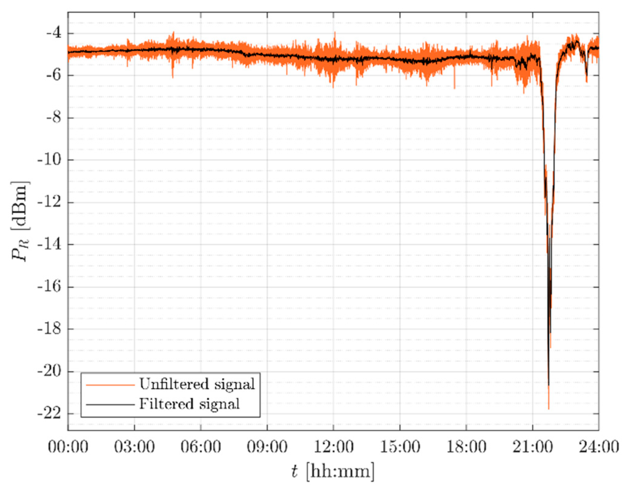
Figure 2.
Low-pass filtered signal (black line) of the Ka-band received signal (orange curve) on 7th September 2017.
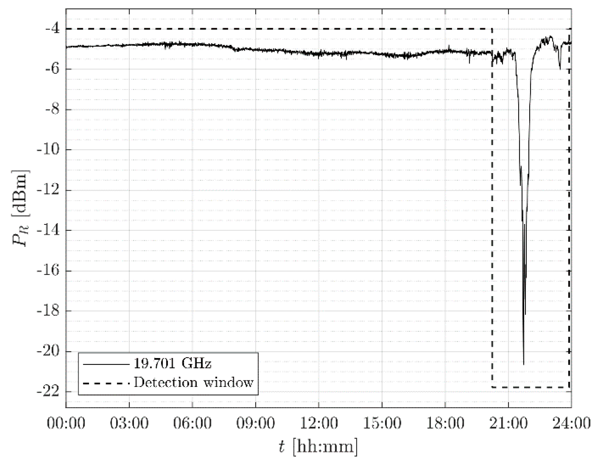
Figure 3.
Detection of the rain event on 7th September 2017.
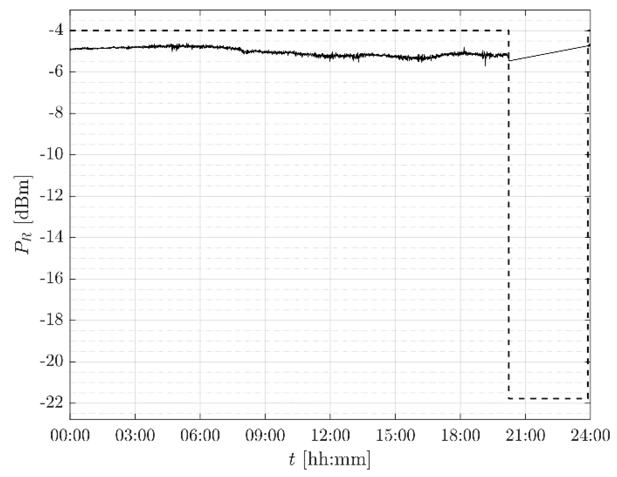
Figure 4.
Reference power level, obtained through linear interpolation during precipitation, for the rain event on 7th September 2017.
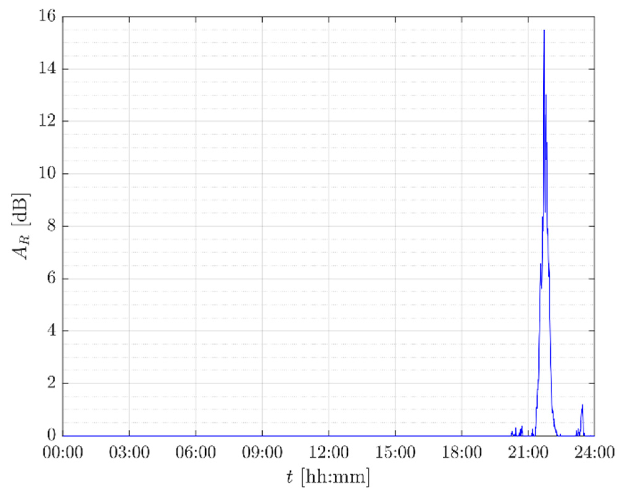
Figure 5.
Rain attenuation time series on 7th September 2017.
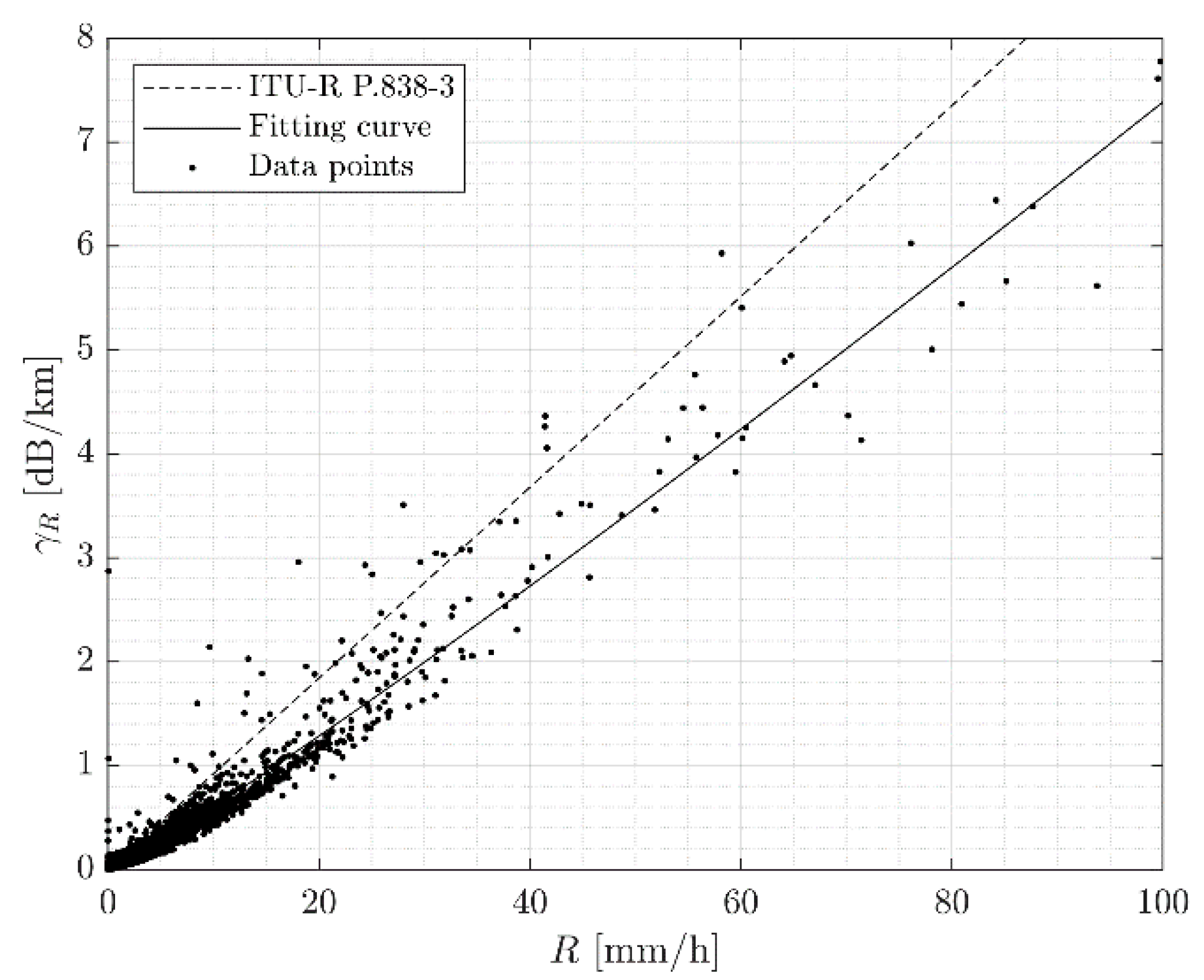
Figure 6.
Specific rain attenuation as a function of the rain rate in Milan (19.701 GHz).
Figure 7.
Comparison between the inverse functions
(dotted lines) and
(continuous lines), using the
and
values reported in the third column of
Table 1.
Figure 8.
Trend of with the month for Milan.
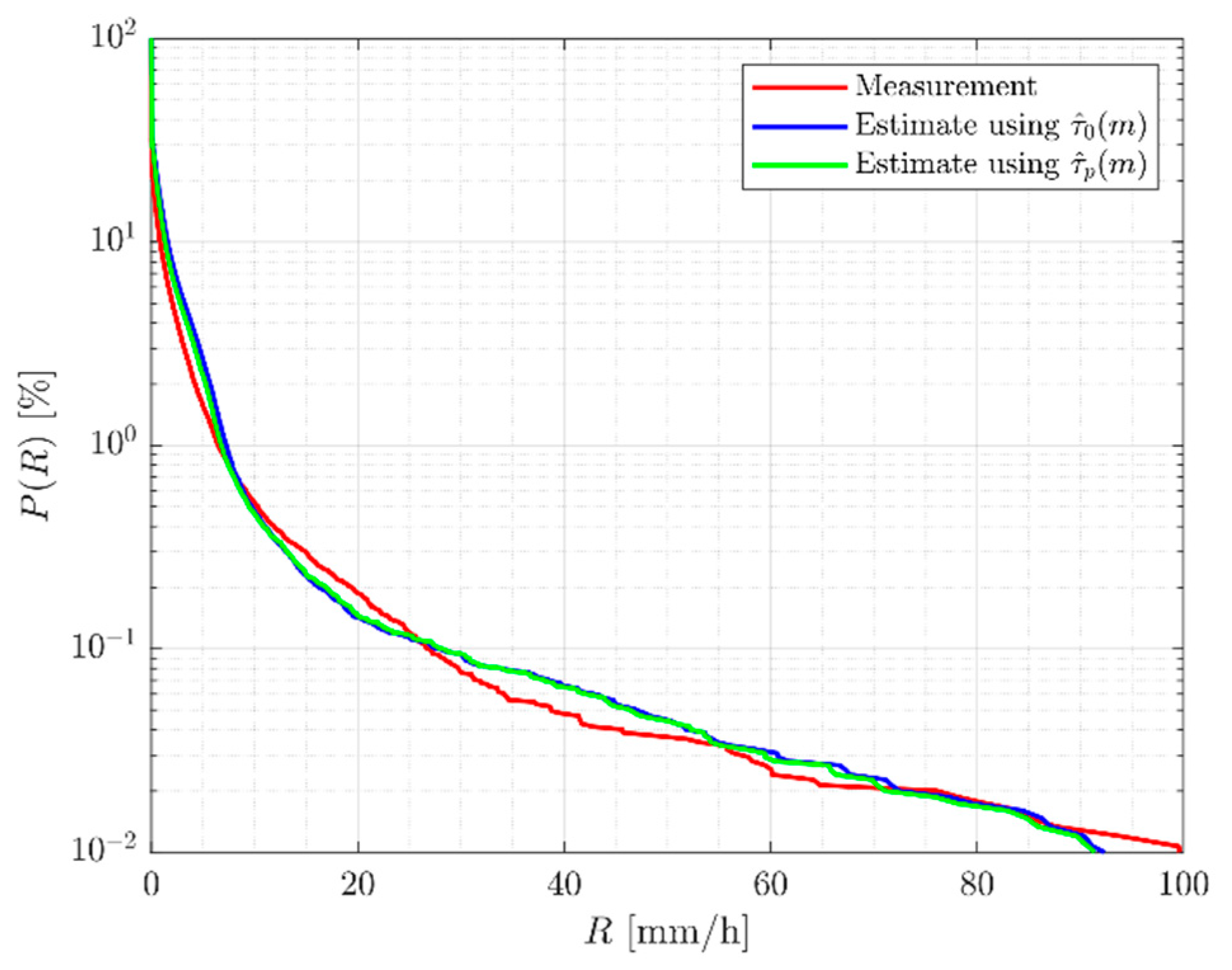
Figure 9.
Comparison between annual rain rate Complementary Cumulative Distribution Functions (CCDFs).
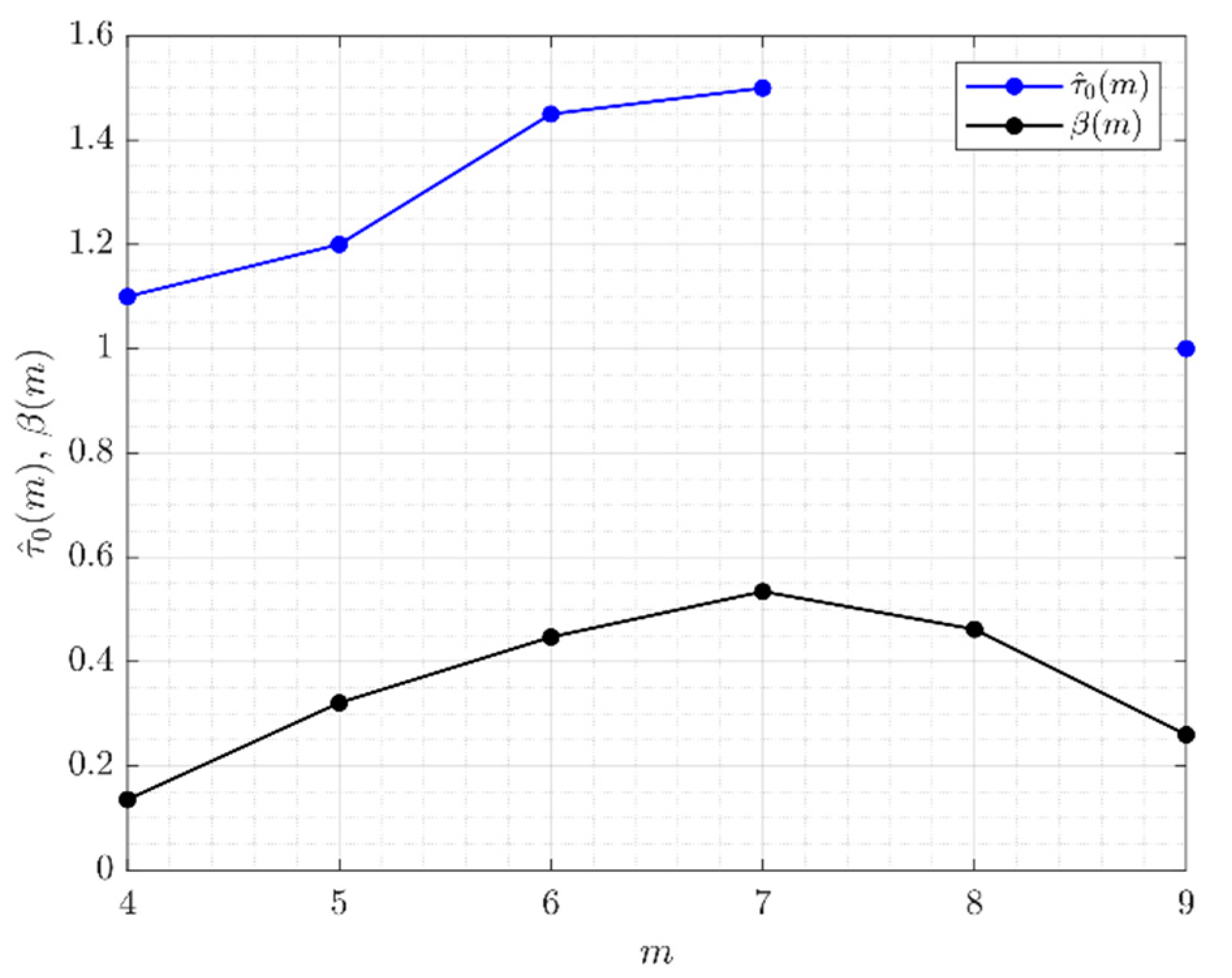
Figure 10.
Trend of and as a function of the month.
Figure 11.
Rain rate time series for the event on 26th April 2017.
Figure 12.
Accumulated rainfall for the event on 26th April 2017.
Figure 13.
Rain rate time series for the event on 25th November 2017.
Figure 14.
Accumulated rainfall for the event on 25th November 2017.
Figure 15.
Trend of the equivalent rain height for the events represented in
Figure 11 and
Figure 13.
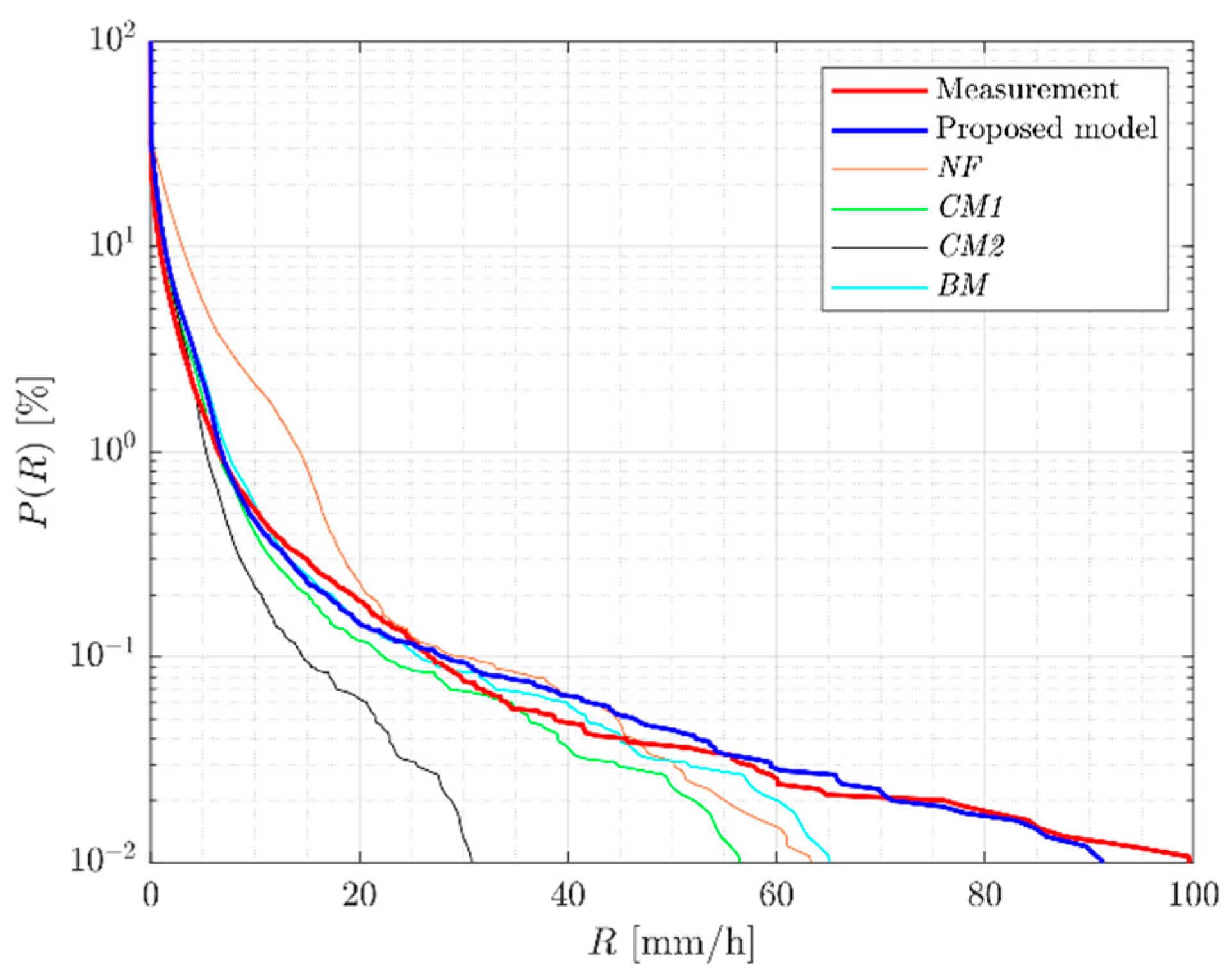
Figure 16.
Yearly P(R): comparison of different models.
Table 1.
and fitting coefficients at 19.701 GHz.
| Coefficient | Recommendation ITU-R P.838-3 | Local DSD Data |
|---|
| 0.0924 | 0.0495 |
| 0.9989 | 1.0870 |
Table 2.
Fitting accuracy for function and .
| Function | | | |
|---|
| | | |
| | | |
| | | |
| | | |
Table 3.
Comparison between different values of .
| | | | | | |
|---|
| | | | | | |
| | | | | | |
Table 4.
Mean and RMS values for the comparison between the curves reported in
Figure 9.
| | | |
|---|
| mm/h | mm/h |
| mm/h | mm/h |
Table 5.
Average (on all the events) of the mean and Root Mean Square (RMS) values of the residuals in (21)–(23).
| Residual | Mean Value | |
|---|
| mm/h | mm/h |
| mm/h | mm/h |
| mm/h | mm/h |
Table 6.
Mean and RMS values corresponding to the comparison between the measurement and the estimated curves reported in
Figure 16.
| Model | | |
|---|
| Proposed Model | mm/h | mm/h |
| mm/h | mm/h |
| mm/h | mm/h |
| mm/h | mm/h |
| mm/h | mm/h |
Table 7.
Average (on all the events) of the mean and RMS values of .
| Model | | |
|---|
| Proposed model | mm | mm |
| mm | mm |
| mm | mm |
| mm | mm |
| mm | mm |
Table 8.
Average (on all the events) of the mean and RMS values of
| Model | | |
|---|
| Proposed model | mm/h | mm/h |
| mm/h | mm/h |
| mm/h | mm/h |
| mm/h | mm/h |
| mm/h | mm/h |
Table 9.
Average (on all the events) of the mean and RMS values of .
| Model | | |
|---|
| Proposed model | mm/h | mm/h |
| mm/h | mm/h |
| mm/h | mm/h |
| mm/h | mm/h |
| mm/h | mm/h |
© 2019 by the authors. Licensee MDPI, Basel, Switzerland. This article is an open access article distributed under the terms and conditions of the Creative Commons Attribution (CC BY) license (http://creativecommons.org/licenses/by/4.0/).


