Article

Multi-Modal Emotion Aware System Based on Fusion of Speech and Brain Information

1
Department of Computer, Mansoura University, Mansoura 35516, Egypt
2
Department of Information Technology, College of Computer and Information Sciences, Princess Nourah bint Abdulrahman University, Riyadh 84428, Saudi Arabia
3
Faculty of Engineering & IT, The British University in Dubai, Dubai 345015, United Arab Emirates
*
Author to whom correspondence should be addressed.
Information 2019, 10(7), 239; https://doi.org/10.3390/info10070239
Submission received: 28 May 2019 / Revised: 26 June 2019 / Accepted: 27 June 2019 / Published: 11 July 2019

Abstract

:
In multi-modal emotion aware frameworks, it is essential to estimate the emotional features then fuse them to different degrees. This basically follows either a feature-level or decision-level strategy. In all likelihood, while features from several modalities may enhance the classification performance, they might exhibit high dimensionality and make the learning process complex for the most used machine learning algorithms. To overcome issues of feature extraction and multi-modal fusion, hybrid fuzzy-evolutionary computation methodologies are employed to demonstrate ultra-strong capability of learning features and dimensionality reduction. This paper proposes a novel multi-modal emotion aware system by fusing speech with EEG modalities. Firstly, a mixing feature set of speaker-dependent and independent characteristics is estimated from speech signal. Further, EEG is utilized as inner channel complementing speech for more authoritative recognition, by extracting multiple features belonging to time, frequency, and time–frequency. For classifying unimodal data of either speech or EEG, a hybrid fuzzy c-means-genetic algorithm-neural network model is proposed, where its fitness function finds the optimal fuzzy cluster number reducing the classification error. To fuse speech with EEG information, a separate classifier is used for each modality, then output is computed by integrating their posterior probabilities. Results show the superiority of the proposed model, where the overall performance in terms of accuracy average rates is 98.06%, and 97.28%, and 98.53% for EEG, speech, and multi-modal recognition, respectively. The proposed model is also applied to two public databases for speech and EEG, namely: SAVEE and MAHNOB, which achieve accuracies of 98.21% and 98.26%, respectively.

1. Introduction

In human–computer interaction (HCI), comprehending and discriminating emotions turned into a principal issue to construct intelligent systems that could perform purposed actions. Emotions can be discriminated utilizing distinct forms of sole modalities, like facial expression, short phrases, speech, video, EEG signals, and long/short texts. These modalities vary over the computer applications, e.g., the well-known modality in computer games is video.
Recent studies unveil several merits of employing physiological signals for recognizing emotions [1]. For instance, the electroencephalogram (EEG) signals have been shown to be a robust sole modality [2,3]. The control of these bio-signals is managed by our central nervous system; thus, it cannot be affected intentionally, while actors can pretend with emotion on their faces deliberately. Further, physiological signals are emitted constantly and since sensors are directly attached to subject’s body, they are not out of reach. Moreover, physiological information could also be utilized as supplementary to emotional information gained from facial expressions or speech to optimize the recognition rates.
In this regard, several multi-modal emotion recognition approaches have achieved significant contributions [4,5,6]. Though there are distinctive input modalities for recognizing emotions, the most widely recognized are bimodal inputs that combine both speech and video. The two modalities have been selected frequently by the researchers because of being captured in a noninvasive way and are expressive than the other modalities. Nevertheless, face expressions might be falsified by not returning accurate information regarding the person’s internal state.
From between the modalities that tend to be in the literature, speech is an intuitive measure for computers to comprehend human emotion, whereas EEG [7] is an internal measurement from the brain that makes an intriguing alternative for recognizing multi-modal emotion. Up until now, there are no proposals that have endeavored to consider speech and EEG simultaneously for recognizing spontaneous emotion. This has motivated us to propose a new multi-modal emotion aware system that fuses speech and EEG modalities for discriminating emotional state of the subject.
In the multi-modal fusion, input information from many modalities, like audio, EEG, video, and electrocardiogram (ECG) can be fused together coherently [8]. More than one modality cannot be combined in a context-free way; a context-dependent model has to be utilized. Information fusion is classified into three progressive stages: (I) Early fusion, (II) intermediate fusion, and (III) late fusion. As for early fusion, integration of information is implemented at signal-/feature-level, while in late fusion, information at a semantic level is to be fused. The foundation in combining multi-modal information is the modalities number [2,3], information derivation synchronization, and fusion procedure, besides finding the proper fusion level of information. However, it is not constantly fundamental that diverse modalities give complimentary information through the fusion stage; therefore, it is essential to comprehend each modality’s contributions with respect to accomplishment of distinct tasks.
One of the important problems faced in the multi-modal emotion recognition is the fusion of features belonging to different modalities. By reviewing the literature on the multi-modal emotion analysis, it has been observed that the majority of works have concentrated on the concatenation of feature vectors obtained from different modalities. However, this does not take into consideration the conflicting information that may be carried by the unimodal modalities. On the other hand, little work has addressed this issue through new feature-fusion methods to enhance the multi-modal fusion mechanism [9,10,11,12].
In [9], the authors proposed a feature fusion strategy that proceeds from the unimodal to bimodal data vectors and later, the bimodal to trimodal data vectors. In [10], a context-aware audio–video system is proposed. Accordingly, a contextual audio–video switching approach is presented to switch between visual-only, audio-only, and audio–visual clues. The proposed approach integrates the convolutional neural network (CNN) and the long-short-term memory (LSTM) network. Moreover, a multi-modal hybrid deep neural network architecture is presented in [11] for audio–visual mask estimation. In [12], an image-text emotion analysis model is proposed. To utilize the internal correlation between the image and textual features, an intermediate fusion-based multimodal model was proposed. Eventually, a late fusion scheme was applied to combine the models of sentiment prediction.
One of the drawbacks of feature-level emotion fusion is that it might exhibit high dimensionality and poor performance because of redundancy and inefficiency. For overcoming the high dimensionality issue, hybrid intelligent models can introduce several choices for unorthodox handling of complex problems, which carry uncertainty, vagueness, and high dimensionality of data. They can exploit a priori knowledge and the raw data to introduce innovative solutions. In this regard, hybridization is a crucial phase in many domains of human activity [13,14].
This paper suggests a new hybrid emotion recognition model based on the fuzzy clustering, genetic search-based optimization. The proposed model selects and trains the neural network (NN) with the optimal fuzzy clusters representing each modality, without any prior knowledge about the fuzzy clusters number. Unlike the previous works on multimodal emotion fusion, the fusion of two modalities is implemented on the decision-level instead of the feature-level fusion that may carry conflicting information. For comparison purposes, the proposed hybrid model is likewise compared to another developed hybrid c-means-genetic algorithm-neural network model, namely, F C M G A N N f i x e d model that relies on defining a fixed fuzzy clusters number.

2. Related Work

This study suggests a novel multi-modal emotion aware system by fusing together speech and EEG modalities. Consequently, the literature review section is progressive. So, the emotion recognition topic of interest is divided into three parts speech emotion recognition, EEG-based emotion recognition, and multi-modal emotion recognition.

2.1. Literature Review on Speech Emotion Recognition

The related work on speech emotions classification reveals three crucial aspects. Firstly, preparing the emotional database is critical to validate the system performance. Secondly, selecting features properly for speech characterization. Eventually, design of accurate classification model. For emotional speech databases, acoustic analysis has been utilized to recognize emotions using three kinds of databases: Natural spontaneous emotions, acted emotions, and elicited emotions.
Most emotional speech databases depend on inviting professional actors for expressing pre-determined sentences related to the purposed emotion. Though, in some databases like the Danish Emotional Speech (DES) database [15], semi-professional actors are invited for avoiding exaggeration during expressing emotions. As for spontaneous speech, databases may be collected from interaction with robots, or call center data.
The performance of the speech emotion recognition system depends on the features extracted from the speech signal. A challenging issue in recognizing speech emotions is extracting speech features that efficiently describe the speech emotional content and, simultaneously, do not rely on the speakers or the lexical contents. The majority of published works on speech emotion classification have concentrated on analyzing speech spectral information and prosodic features. Some new parameters are utilized for recognizing speech emotion, like the Fourier parameters [16]. Although numerous acoustic parameters have been found to carry emotional content, little success was proved to define a feature set that performs invariably over diverse conditions [17].
Therefore, the majority of works use mixing feature set, which comprises several types of features involving more emotional information [18]. This is implemented by dividing the signal into k frames/segments containing n samples per frame/segment, which causes a high dimensionality problem. As a result, the computational cost and over-fitting likelihood of the speech classifier are increased. Thus, feature selection approaches are imperative to minimize feature redundancy and speed up the learning process of speech emotion recognition.
Table 1 [19,20,21,22] summarizes some works on speech emotion recognition. By reviewing these works, it is obvious that the most used classifiers are artificial neural networks, Gaussian mixture model, and multiple different one-level standard methodologies. Satisfactory outcomes are obtained using these standard classifiers. Nevertheless, the improvements in their performances are usually restricted. Thus, the fuzzy genetic search-based optimizations and fusion of speech classifiers could constitute a new step toward robust emotion classification [23,24]. Therefore, we hypothesize that the proposed hybrid soft computing model can overcome the existing limitations of speech emotion recognition.

2.2. Literature Review on EEG-Based Emotion Recognition

The initial stage of EEG-based emotion classification is to take accurately labeled EEG signals induced by picture, video clips, or music. Subsequent to presentation of visual stimuli to a subject, multi-channel signals of EEG are recorded, and afterwards, the signal labeling is done based on subject ratings. The previous work on EEG emotional features extraction [25,26,27,28,29] has revealed that there exist several valuable features of time, frequency, and time–frequency that have been evidenced to be efficient in differentiating emotions. Furthermore, there is no standard feature set that has been agreed as the most appropriate for EEG emotion classification. This causes a high dimensionality issue in EEGs, because not all features would contain significant information concerning emotions. The redundant and irrelevant features maximize the feature space, making the detection of patterns more difficult, and maximizing the over-fitting risks.
However, the majority of classifiers that have been proposed in the literature for EEG emotion classification are based on the conventional classification algorithms such as ANN, SVM, and k-nearest neighbor. Some of these approaches are demonstrated in Table 2. Few works have presented hybrid methods of evolutionary computer algorithms and classification methods [25], where the objective of these works is to deal with the high dimensionality issue of EEG emotion recognition. Therefore, in this work, we propose a novel fuzzy c-means-genetic algorithm-neural network (FCM-GA-NN) model for EEG emotion recognition. The meta-heuristic can provide the optimal initial centroids for the FCM algorithm, which will be trained to the NN as optimized solutions for emotion recognition. In this regard, the proposed algorithm has been experimented on our collected database and another publicly available database, namely MAHNOB. The comparative results are demonstrated in the experimental results section.

2.3. Literature Review on Multi-Modal Emotion Recognition

Recently, a little work has investigated multiple modalities to recognize emotions [9,10,11,12]. Many studies have fused facial expression together with physiological signals [30]. Table 3 [30,31,32,33] presents some of the surveyed studies on the multi-modal emotion fusion, including the corpus, modalities of fusion, feature extractors, fusion approach, classifier, and classification accuracy. As indicated in the literature and to the best of our knowledge, there are no works reported on fusing speech with EEG for recognizing emotions. Furthermore, the resulting accuracies are still below expectations.
It is also observed that the large number of multi-modal emotion fusion works is based on the feature-level fusion that concatenates the features obtained from the signals of multiple modalities before feeding them to the classifier. This may exceed the risks of conflicting information that may be carried by the sole modalities. On the other hand, a little work has been implemented on the decision-level fusion, which attempts to manipulate each sole modality separately, and integrates later the results from their classifiers for making the final recognition.
In the two cases of multi-modal emotion fusion, the high dimensionality or the redundant features resulting from the processing of each modality may make the learning process complex for the most used machine learning algorithms like the NN classifier, which will be optimized in this work. The training step of NN classifier is a crucial procedure. A high computational time is needed if NN is trained by high-dimensional data. It presupposes network architecture of a huge input layer, which significantly maximizes the weights number, usually causing an infeasible training.
This issue could be solved by minimizing the input space dimensionality to a manageable size, then a network is trained on fewer dimensions. Clustering is a strictly necessary solution that has been exploited to make the dimensionality reduction of an NN training data through organizing group of objects or patterns into clusters. Accordingly, objects within the cluster itself reveal common attributes and others within different clusters reveal dissimilarity. k-means [34] and FCM [35] are the most employed clustering algorithms to train NN. As for FCM, a soft partitioning is executed as a pattern and is esteemed as a member of all clusters, but distinct membership degrees are set for distinct clusters. Despite that, the two algorithms are centroid-based, so they previously assume a fixed cluster number, and are fully sensitive for centroid initialization [36].
On the contrary, several problems do not have knowledge on the clusters number a priori. Numerous studies suggested solutions for these problems through running the algorithm repeatedly along with diverse fixed centroid value k and with diverse initializations. Nevertheless, this might not be doable with the big datasets. Moreover, running the algorithm through using a limited centroid number might be inefficient because one solution relies on a limited initialization set. This is referred to as “clusters number dependency” issue [37].
For solving this issue, evolutionary approaches reveal alternative optimization approaches utilizing stochastic principles for evolving clustering solutions. They also are based upon probabilistic rules for returning the near-optimal solution among the global search space. A few evolutionary methods have been suggested for optimizing clusters number in data partitioning issues [38,39]. In [38], an algorithm of artificial bee colony was executed to mimic an intelligent foraging conduct of honey bee swarms. In [40], a k-means was optimized through a GA, which esteems the impact of isolated points. Several studies also suggested a number of approaches for NN optimization by GA [41,42,43,44].
To overcome the high dimensionality issue, this paper suggests a new multi-class NN model, which is optimized by hybridization of the FCM and GA. For each sole modality, the GA selects the optimal centroids for the FCM algorithm. Then, the NN is automatically trained with the optimized solutions from each modality, which reduce the classification error without any prior knowledge about the fuzzy clusters number. For comparison purposes, we developed another hybrid model of FCM, GA, and NN, which is trained using a fixed number of fuzzy clusters. The fusion is then implemented on the decision level.

3. Proposed Methodology

The proposed system architecture is as depicted in Figure 1, which comprised five steps: (i) Multi-modal data acquisition, (ii) pre-processing, (iii) feature extraction, (iv) classification using the proposed hybrid fuzzy c-means-genetic algorithm-neural network model (CM-GA-NN) model, and (v) fusion on the decision-level. Speech and EEG signals are acquired from subjects simultaneously. Recorded signals are then pre-processed to eliminate noise of external interferences. Next to pre-processing, some speaker-dependent and -independent features are estimated from speech signals. For EEG signals, features are estimated from three domains: Time, frequency, and time–frequency. For classifying unimodal data (speech and EEG), the proposed hybrid FCM-GA-NN model is used. To fuse speech and EEG information, two algorithms are experimented, where a separate FCM-GA-NN classifier is used for each modality, then the output is computed by integrating posterior probabilities of sole modalities.

3.1. Multimodal Data Acquisition

There are a number of multi-modal emotional databases that comprise either speech or facial expressions with different types of physiological signals. However, to the best of our knowledge, there are no available databases that integrate both speech and EEG information. The details about multi-modal data collection could be found in [45]. In the literature, there are different types of stimuli that have been utilized by the researchers to induce emotions. In [7], different genres of music were chosen as stimuli for inducing EEG-based emotions. In [46], a hypermedia system, namely MetaTutor, was utilized as stimuli for students learning about a complicated science topic.
To collect the multi-modal data in the current study, the subjects were 36 girls from the College of Computer and Information Sciences, Princess Nourah Bint Abdulrahman University (PNU) for girls, KSA, who voluntarily participated. Their ages range was between 18 and 20 years. The subjects are all Arabic native speakers. The study with its methodology was implemented under institutional ethical review of the University. The steps of the research ethics approach that we adopted are applied as follows:
  • Before the experiment, students were informed of the experiment purpose, and each completed a consent form subsequent to an introduction about the steps of simulation.
  • Identities of subjects were kept anonymous and confidential, where the personal information will not be ever associated or disclosed with any answer.
  • Information acquired from subjects was employed only for the aim of the current research.
  • The accuracy and suitability of health and medical information used in current research were confirmed by experts.
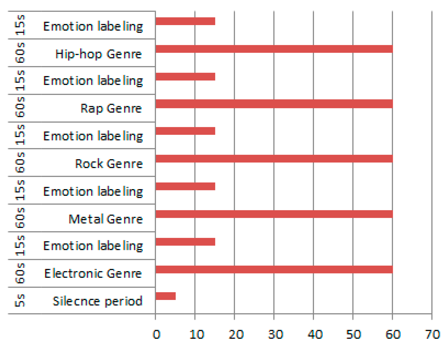
The materials involved 35 music tracks, which were employed as external stimuli for inducing emotions. The English music utilized in this research involved 5 genres: Namely, electronic, metal, rock, rap, and hip-hop. These genres are considered to cover a range that produces discernable emotions. Each participant listened to 7 songs from each genre used (one by one); each of which was followed by 15 s of silence in order to allow for emotion labeling. In this context, the total number of tracks that every participant listened to was 35 (5 genres × 7 songs, each of which represents a type of emotion classes), as demonstrated in Table 4.
Only 60 s of every song was employed to avoid inducing anxiety and boredom in a participant's brain, as depicted in Figure 2. The subjects annotated their emotional status by the end of each music track picking one of the seven available emotional keywords: Fear, surprise, happy, disgust, neutral, anxiety, and sadness [7,45]. To avoid the participant’s subjectivity and exaggeration while expressing emotions, the experiment was also noticed by an expert of psychology who judged through listening to the participant’s emotional speech and did the final labeling of emotions to exclude the spoofed labeled emotion. According to the keyword used by the subject and the evaluation of the expert, the approved speech/EEG recording was mapped to its representative class. Otherwise, the unapproved one was excluded.
While the participants were listening to the music tracks through headphones, the speech and EEG signals were acquired simultaneously. The speech signals were acquired spontaneously using a microphone, namely: “SHURE dynamic cardioid microphone C660N”. The distance from microphone to speaker was kept at 3 m. The speech signals were sampled at 16 KHz. For Arabic speech signal acquisition, each subject had to describe the feeling induced while listening to the audio i.e., “أنا مكتئبة جداً/I am feeling deep depression”.
Likewise, the EEG recordings were taken using the Emotiv-EPOC System. The device involves 14 electrodes together with 2 reference channels, which present accurate spatial resolution. The inner sampling rate of the device was 2048 Hz prior to filtering, and its output sampling equaled 128-samples/second. The electrode placement was chosen as 10/20. This placement is commonly used in studies for EEG-based emotions recognition using visual and audio stimuli. This system relies on relationships of diverse electrode positions existing on the scalp as well as the main cerebral cortex side [38]. Figure 3 depicts the 16 electrodes, “AF3, F7, F3, FC5, T7, CMS, P7, O1, O2, P8, DRL, T8, FC6, F4, F8, and AF4”, which were embedded to the record of the EEG signals. In the locations of P3/P4, the channels of average reference (CMS/DRL) were situated. The MATLAB and Puzzle box synapse were utilized for recording signals of Emotiv EPOC headset.
The data collection was implemented during the analysis [7], by using only the parts of speech and EEG data that the subjects were listening to music through, leaving out the parts of annotation. In this regard, 1260 speech samples, as well as 1260 EEG signals, were acquired from students. Thus, the total number of samples within our multi-modal emotional database was 2520. The duration of each speech/EEG signal was 60 s. Characteristics of the corpus and its statistics are demonstrated in Table 4, where emotions are sorted by arousal and valence dimensions [46], along with the representation of their classes in the corpus.

3.2. Speech Signal Pre-Processing

To identify diverse speech multi-styles and emotion states, silent features had to be isolated. As the recorded signals are of distinct sampling frequency rates, we down-sampled all signals to 8 KHz. Then, signals were sub-divided into non-overlapping segments (frames) of 32 ms (256 samples). This frame length gave the best performance in this paper. According to [47], the unvoiced parts are eliminated from signals based upon existing energy within the frames and the frames with lower energy are eliminated before the feature extraction takes place. The speech segment (of 256 samples) was classified as voiced, unvoiced, or silence by computing its discrete wavelet transform (DWT) at scales m = 2 1 through m = 2 5 and computing the signal energy over each scale. Then, a decision scheme based on scale-energy was employed for detecting voiced speech segments.
As the unvoiced speech is of a high frequency nature, its DWT energy was high at scale m = 2 1 . Thus, this method determines the scale at which the DWT of signal reaches the highest energy. The segment is considered unvoiced if its DWT reaches its highest energy at scale m = 2 1 . Otherwise, it may be a silence or voiced segment relying on its energy over the higher scales. Accordingly, the DWT energy over the scale m = 2 3 of each segment, which was not classified as unvoiced, is compared to a predefined threshold. Thus, the segments that exceed this threshold are classified as voiced. Otherwise, they are classified as silence.
According to [24], the median of segment energies over the scale m = 2 3 gives a good criterion for discriminating the silence speech signals from the voiced ones. Thus, the threshold used in this regard was the median of segment energy distribution at the silence and voiced speech segments computed over scale m = 2 3 . The other voiced frames were then concatenated and the glottal waveforms were obtained using inverse filtering as well as linear predictive analysis approach. The resulting speech and glottal waveforms were filtered utilizing a 1st-order pre-emphasis filter [24] expressed by Equation (1). The parameters of such filter were set as in [48].
H ( S ) = 1 a S 1 0.9 a 1.0
where S the speech signal and a takes a value of 0.9375.

3.3. EEG Signal Pre-Processing

EEG signals comprise multiple extrinsic and intrinsic artifacts that obscure the waves of brain. Extrinsic artifacts (i.e., wiring noise of the EEG sensor) have different frequencies that may interfere with the brain waves. Eliminating these artifacts requires filtering frequencies that are out of EEG signals scope. Accordingly, we employed a band-pass filter with 64 Hz and 0.5 Hz of the maximum cutoff frequency and the minimum cutoff, respectively [49]. Likewise, the notch filter that filters out the signal narrow frequencies band [50], was utilized for noise isolation from the ambient electrodes' wire resulting from the signal of power line interference (i.e., 60 Hz).
To isolate intrinsic artifacts, the independent component analysis algorithm is employed to determine artifactual elements (i.e., blinking, eye movement) found in EEG recordings. This algorithm eliminates intrinsic artifacts from signal without loss through determination of the artifactual EEG elements and subtraction of the elements, which are associated with intrinsic artifacts for obtaining a cleaner EEG signal. It has also been frequently utilized in EEG clinical studies for detecting and eliminating intrinsic artifacts [51].

3.4. Speech Feature Extraction

Recently, most of the speech emotion recognition systems shown in the literature are trained only using a specific emotional database of particular persons. This may cause drawbacks like the lake of generality. As a result, the emotion recognition accuracy of any person who does not belong to this database will be low. Thus, eliminating the speech individual difference is the primary step to enhance the speech emotion recognition accuracies and the system universality. In this stage, feature extraction is implemented after dividing the speech signals into a sequence of non-overlapped sub-frames/segments, each of which has a length of 256 samples. Then, the speaker-dependent and speaker-independent features [20,21,52] are computed from each frame as follows. The selected features have been shown in the literature to carry an important emotional content [20,21,52].
(a)
Speaker-dependent features: Usually involve valuable personal emotional information [52], as demonstrated in Table 5. They comprise fundamental frequency, fundamental frequency four-bit value [20], Mel-frequency cepstral coefficients (MFCC), etc.
(b)
Speaker-independent features: These features are used to suppress the speaker’s personal characteristics. In [20], the speaker-independent features from emotional speech involve the fundamental frequency average change ratio, etc.

3.5. EEG Feature Extraction

In this paper, we use a mixing set of EEG features that have been proven in the literature to be highly effective in emotion recognition [26,29]. These features belong to time, frequency, and time–frequency. The EEG signal is blocked into windows/frames. From the literature, the efficient window size ranges from 3 to 12 s, when classifying the individuals’ mental state utilizing EEG signals [53]. Two methods of windowing i.e., fixed windowing and sliding windowing, were tested to choose the superior method in reference to classification accuracy. In this paper, we estimate 23 measures of time, frequency, and time–frequency presented in Table 6, from 14 EEG channels.

3.6. The Classifier

3.6.1. The Basic Classifier

NN is a parallel processor distributed massively [41]. It involves single input layer, besides one output layer, as well as one hidden layer. Such a hidden layer is like a connection in between input/output layers through multiple weights, nodes, biases, in addition to activation functions. The operational procedure of NN is denoted by the subsequent equations:
W j = t = 1 k ω j t X t
Y j = ϕ ( W j + A j )
where j indicates a neuron in the network, k is input parameters number, X t ( t = 1 , 2 , , k ) represents the t-th input parameter, in addition to ω j t ( t = 1 , 2 , , k ) , denotes respective synaptic weight. Initially, every synaptic weight ω j t multiplies the input sample X t , which conforms to it. Values of weight are put in a summator , getting an output, indicated as W j . Afterwards, W j is applied to the activation function ϕ for producing an output signal Y j , and A j denotes the bias.
This study deals with a multi-class classification problem where N classes of emotions are to be recognized. According to the literature [54], the multi-class neural network (NN) classification can be implemented using: (1) Either a single neural network model with K outputs or (2) a multi-NN model with hierarchical structure. In this regard, there are two methods that can be employed to model the pattern classes, one-against-all (OAA) approach, and one-against-one (OAO) approach [54,55,56].
In this paper, we present a multi-class back propagation neural network for emotion classification. We adopt the OAA approach scheme, which operates on a system of M = N binary neural networks, N N j , j = 1 , , N , where each single network, N N j , holds one output node P j that has an output function F j being modulated to output F j ( x ¯ ) = 1 o r 0 to determine whether or not the input sample x ¯ belongs to class j . Accordingly, each neural network N N j is trained using the same dataset but with different class labels.
For training the j t h neural network N N j , the training set Ω T is subdivided into two sets, Ω T = Ω T j Ω ¯ T j , where Ω T j includes all the class j samples, which obtain the label 1 , and Ω ¯ T j includes all the samples belonging to all of the rest classes, which obtain the label 0 . The decision function considers the activation function output at every neural network N N j , and outputs the label of the class that confronts to neural network N N j , which obtains the highest output value by the activation function of the Pj output node:
F ( x ¯ , y 1 , , y M ) = a r g   m a x j = 1 , , M ( y j ) .
In this study, we constructed an OAA system of 7 binary NNs with 20 hidden nodes for each of which. Selecting the appropriate parameters for the multi-class back-propagation neural network was based upon minimizing the root-mean-square-error (RMSE) between target and the predicted output. The parameters giving the best accuracy are demonstrated in Section 4.

3.6.2. Proposed Classifier Design

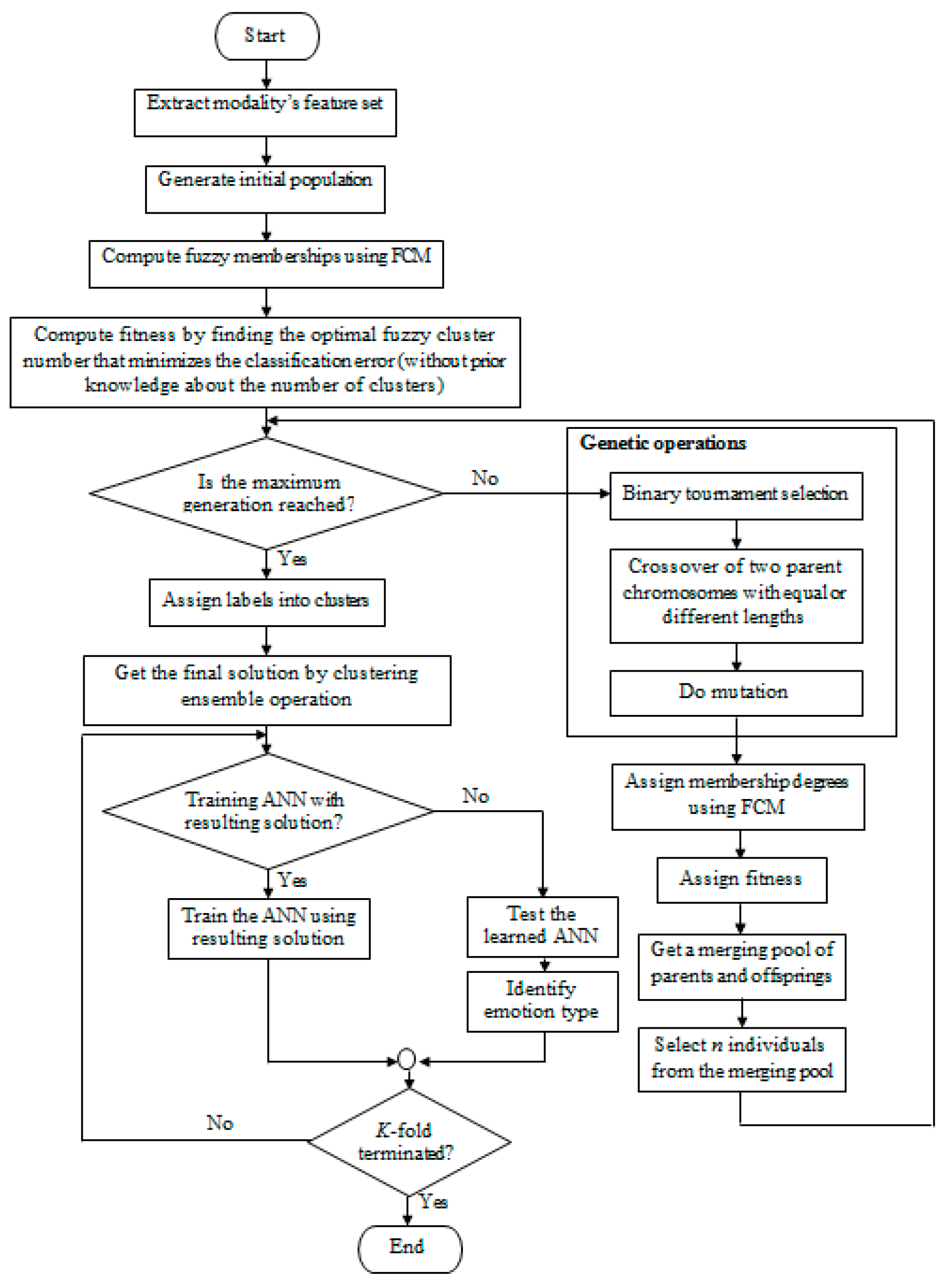
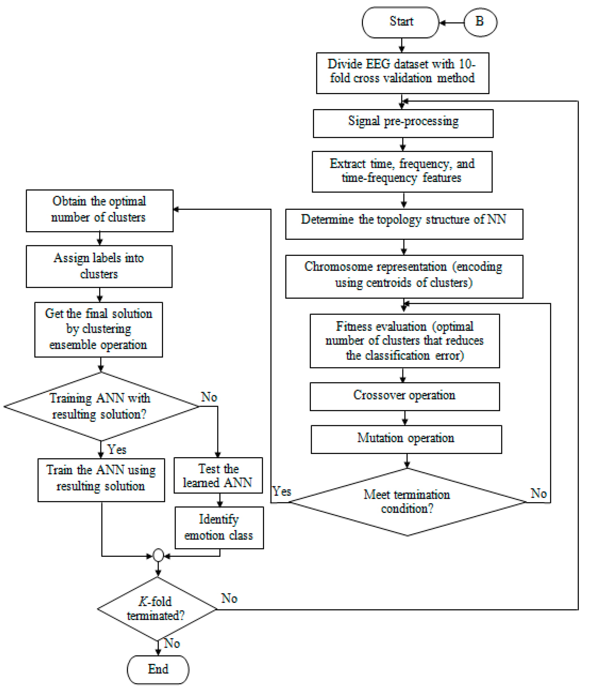
The proposed hybrid FCM-GA-NN model is depicted in Figure 4. The chromosome fitness (feature selection outcome) is evaluated based on the optimal fuzzy clusters that reduce the NN classification error with no prior knowledge about the number of fuzzy clusters. Thereafter, chromosomes are encoded utilizing the resulting fuzzy memberships. Since the cluster number u is not determined, the population may have chromosomes with uniform or different lengths. Therefore, a modified single-point crossover algorithm is developed. Accordingly, the mutation algorithm changes every dimension of a solution by a probability P T . Then, the fuzzy memberships are computed, and the clustering indices of the object are taken based on the maximum fuzzy membership values respecting different fuzzy clusters. In this regard, some empty classes may be found when crossing two parents of different lengths, or if a class number is of big size. In case of an empty j-th class, the center u j will be eliminated from { u 1 , u 2 , , u J } . Update of the new memberships and centroids with the remaining centroids is accordingly implemented. In the last generation, the algorithm generates a non-dominated set of solutions whose number changes in reference to population size. Such solutions are regarded as equal in relation to the fitness values obtained by fitness function. The final clustering outcome is determined based upon a clustering ensemble method. Algorithm A1 reveals the pseudo-code of the whole proposed model Appendix A.
The steps of the proposed algorithm are as follow:
(a) Fuzzy-clustering of each modality’s emotional dataset
The purpose of a clustering algorithm goes to separation of resembling objects, i.e., feature vectors into shared cluster and unalike objects into distinct clusters; thus, the within-cluster objects similarity measure is large and is contrarily small for the between-cluster objects. In this paper, each modality’s feature set is separated into training and testing sets. Consequently, the FCM algorithm is executed to cluster the relevant emotion vectors in each modality’s training set individually into several categories, i.e., emotional speech classes as well as emotional EEG classes. The developed clustering procedure is demonstrated in Equations (5)–(9) of Algorithm A2,
i = 1 u μ i , k m = 1 , k = 1 , 2 , , K
0 < k = 1 K μ i , k m < K , i = 1 , 2 , , u
R i m = k = 1 K ( μ i , k m ) a x k k = 1 K ( μ i , k m ) a , i = 1 , , u , 1 < a
μ i , k m + 1 = [ h = 1 u ( | | x k R i m | | 2 / | | x k R h m | | 2 ) 1 a 1 ] 1
K a m + 1 = k = 1 K i = 1 u [ ( μ i , k m + 1 ) a | | x k R i | | 2 ]
where:
  • K the number of emotional classes in each modality’s dataset,
  • x k the emotion feature vector of the sample k ,
  • μ i k m the emotion feature vector’s membership grade belonging to cluster i at time m , 0 < k = 1 K μ i k m < K ,
  • ε decides time complexity and precision for clustering. (in this paper, it was set as 10 10 ).
(b) Chromosome representation
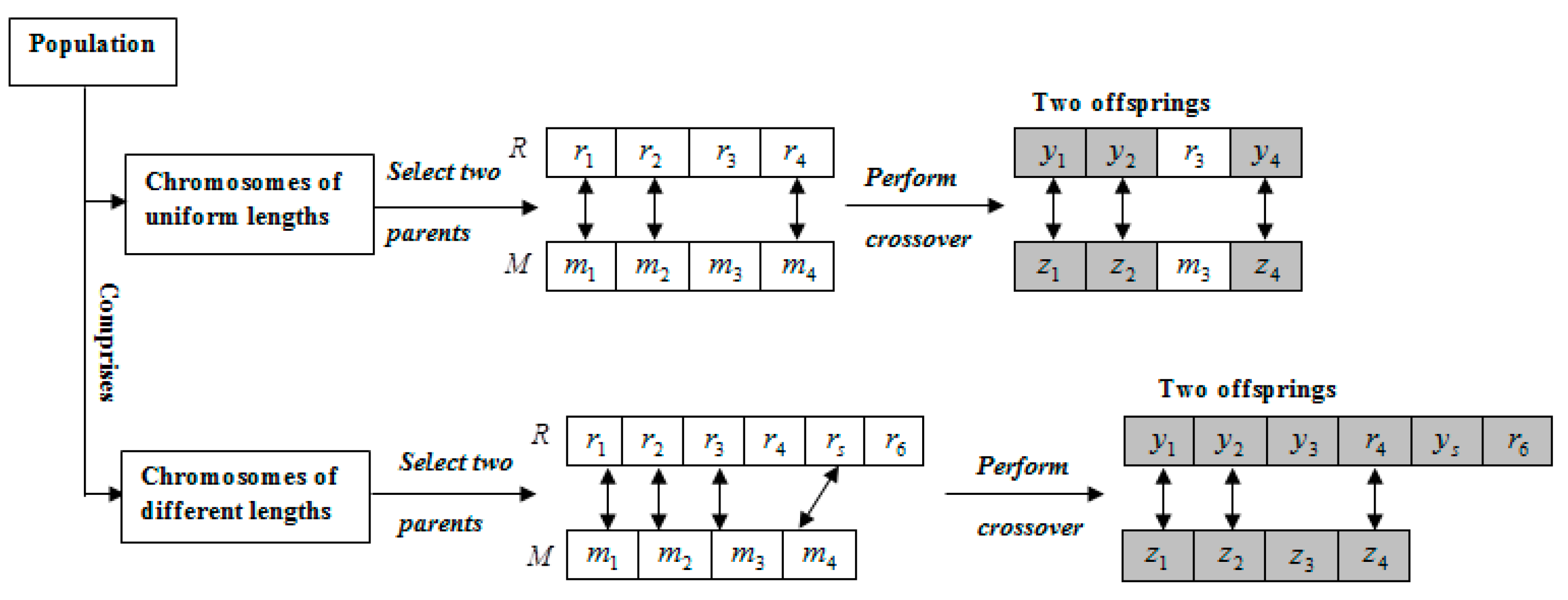
After applying fuzzy clustering, a c × b matrix, representing fuzzy cluster centers, can be considered as a chromosome in GAs terminology. Every chromosome’s gene is indicated by an element of U of Equation (10). To express the decision variables, a matrix U is transformed into a vector = [ B 11 , , B K 1 , . . , B 1 n , , B K n ] , which is encoded as a single chromosome whose length is changing according to n (see Figure 5).
U = [ B 11 B 12 B 13 B 1 n B 21 B 22 B 23 B 2 n : : : : B K 1 B K 2 B K 3 B K n ]
(c) Fitness evaluation
Applying the FCM algorithm attempts to determine optimal number of clusters, that is, for cluster validity. The WB index [57] is utilized to find cluster number u that diminishes the intra-cluster variance a c v ( μ , R ) and increases the inter-cluster variance. On this basis, the feature selection result (the fitness) of the chromosome is assessed by finding the optimal fuzzy clusters that minimizes the classification error without prior knowledge on the clusters number.
To handle that multi-criteria decision-making issue, we used a standalone weighted fitness function combining two single processes into one objective. According to Equation (11), two predefined weights W u and W c are associated with optimal number of clusters u p and classification error , respectively.
F i t F C M G A N N = W u [ u p ] + W c [ c e ]
The optimal cluster number u p is obtained by:
u p = a r g   m a x u   W B = e c v ( μ , R ) a c v ( μ , R )
where:
a c v ( μ , R ) = i = 1 u k = 1 K ( U i ) 1 | | x k R i | | 2
e c v ( μ , R ) = 1 U 2 u λ = 1 u 1 a = λ + 1 u ( U i ) 1 * ( k v λ v a ( μ λ k μ a k ) | v λ | + | v a | ) 1 | | R λ R a | | 2
U i = k = 1 K μ i k 2 / | v i | , i = 1 , 2 , , u
v i = { k | I i k = 1 } ,   I i k = { 1 , f μ i k = max μ h k 1 h u 0 , o t h e r w i s e
and U 2 u indicates a combination computation.
The classification error is computed using:
c e = N E N T
where N E the number of incorrectly classified samples. N T the total number of training instances.
(d) Binary tournament selection
Binary tournament selection technique [58] is utilized in this work to choose parents for creating new generation. Accordingly, two individuals are picked haphazardly for playing a tournament. During that, the winner is picked by n , referred to as a crowded comparison operator. Such operator relies on two attributes denoted as non-domination rank ( A r a n k ) and crowding distance ( A d i s t ). If A and B are assumed to be two individuals, n can be defined as follows. In applying this approach, chromosomes of 40% top-ranking are picked for producing the child chromosomes through crossover and mutation procedures.
A n B i f ( A r a n k < B r a n k ) o r ( A r a n k = B r a n k ) a n d ( A d i s < B g i s t )
(e) Crossover procedure
In this framework, the length of every chromosome within the population is denoted by K × n . The two parent chromosomes might be with equal or unequal lengths relying on the K values; therefore, each cluster centroid may be indivisible while crossing two parents. Thus, a modified single-point crossover algorithm is developed in this paper.
Assuming that R = { r 1 , r 2 , r 3 , r 4 } and M = { m 1 , m 2 , m 3 , m 4 } are two parent solutions having four cluster centers, where each r i and m i represents a feature vector, D 1 and D 2 are two children created. To perform uniform crossover, each two centers from parents are crossed with a probability of 0.5. As depicted in Figure 6, the crossover is not implemented to gene 3, and values of r 3 and m 3 are copied to gene 3 of children D 1 and D 2 , respectively. Values of genes 1, 2, and 4 have been updated to y 1 , y 2 , y 4 and z 1 , z 2 , z 4 on D 1 and D 2 , respectively. If the two parents are with different lengths (see Figure 6), the centroids considered for crossover in the longer parent are randomly picked. Thus, r 1 , r 2 , r 3 , r 5 are chosen and crossed with m 1 , m 2 , m 3 , m 4 , respectively. Then, the omitted centers values ( r 4 , r 6 ) are copied to an offspring. Algorithm A3 demonstrates the crossover procedure between parents. The new centers’ values for two offspring are calculated using Equations (19)–(20) of Algorithm A3.
D j 1 = [ ( 1 + b e t a ) Q 1 + ( 1 b e t a ) Q 2 ] 2
D j 2 = [ ( 1 b e t a ) Q 1 + ( 1 + b e t a ) Q 2 ] 2
(f) Mutation procedure
In this procedure, a small probability of mutating P T is assigned to each gene, determined by randomly generating a number (the gene is mutated if the generated number is less than P T , otherwise not). According to this framework, a change of a gene within a chromosome will trigger a sequence of gene changes. Thus, the fuzzy memberships of a chromosome point will be chosen to mutate together using a probability P T . The mutation procedure is demonstrated in Algorithm A4.
(g) Obtaining final solution
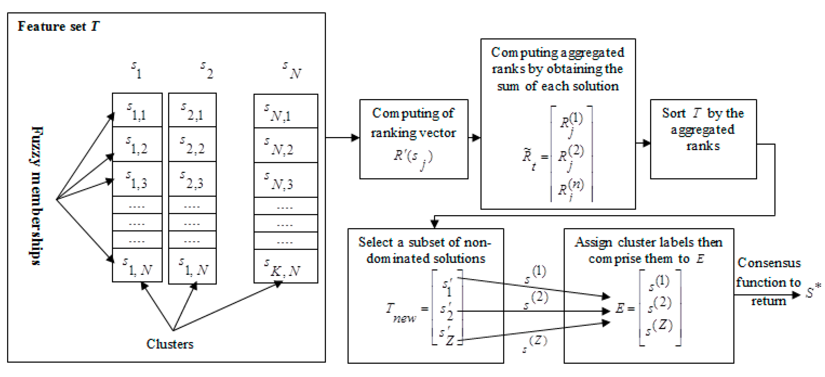
The cluster validity indices are utilized by taking their ranking numbers, so we can choose some solutions to integrate. The ranking of every cluster validity index is illustrated as follows. Assuming the cluster validity indices number is V , a corresponding ranking vector of every solution is R ( s ) = ( r 1 ( s ) , r 2 ( s ) , , r V ( s ) ) , r j ( s ) { 1 , 2 , , n } , 1 j V . Besides that, the sum of cluster validity indices for every solution s is computed. Accordingly, the sum ranking number for every solution is computed as r s u m ( s ) { 1 , 2 , , n } , which is integrated to R ( s ) for generating a new vector referred as R ( s ) = ( r 1 ( s ) , r 2 ( s ) , , r V + 1 ( s ) ) .
Therefore, a total ranking number of s is R t ( s ) = j = 1 V + 1 r j ( s ) . The smallest value of R t may be V + 1 if all cluster validity indices for a single solution are the best. Algorithm A5 shows the steps to get final clustering solution. The whole process is illustrated in Figure 7. Many clustering ensemble algorithms have been compared in the literature [59]. As the meta-clustering algorithm showed the highest performance in terms of accuracy average rates (AVR), it has been applied in Step 13 of Algorithm A5.
(h) Decision-level fusion
A decision-level fusion first processes every modality separately, and then integrates the outcomes from their classifiers to reach the final decision. Motivated by [60], for every trial, assume that M S p e e c h x , M E E G x and M 0 x [ 0 , 1 ] denoting the probability of classifier for class x [ 1 , 2 , 3 ] for speech, EEG, and fusion, each in order. Subsequently, the class probabilities are obtained using
M 0 x = β M S p e e c h x + ( 1 β ) M E E G x
where β is a modality weight. Subsequently, we tested two approaches to calculate β .
Equal weights fusion method (EWF) that makes fusion on a decision-level, where each class final probabilities are estimated using the class probability taken from every sole modality. That is,
M 0 x = M S p e e c h x + M E E G x .
Learned weights fusion method (LWF) is a different method for the decision-level fusion, where an optimal decision weight from each modality is numerically approximated. This is implemented by changing from 0 to 1 and selecting the value that outputs the superior accuracy for the training set. Then, an estimated weight is implemented to the sample, by Equation (22).

4. Experimental Results

This section discusses how the system is evaluated and compared to the state-of-the-art systems. For testing the proposed FCM-GA-NN model performance, we not only conduct our experiments on the collected multi-modal emotion database, but also on two different public unimodal datasets speech and EEG, which are used in the literature for the purposes of comparisons.

4.1. Performance Evaluation Metrics

In this paper, the performance is assessed through four criteria: AVR, root mean squared error (RMSE), percent deviation (PD), and correlation coefficient ( ρ ) . Accuracy is referred to as a truly classified samples ratio, T over the total samples number considered for classification, N . The RMSE is employed for measuring the difference between both predicted and actual values. The correlation coefficient reveals the degree of approximation between estimated and actual values. Calculating the aforementioned indicators is as follows:
A V R = T N
R M S E = 1 N u m i = 1 N u m ( μ x μ y ) 2
P D = 1 N u m i = 1 N u m | μ x μ y | μ x × 100
ρ = i = 1 N u m ( μ y μ Y ¯ ) ( μ x μ X ¯ ) i = 1 N u m ( μ y μ Y ¯ ) 2 i = 1 N u m ( μ x μ X ¯ ) 2 .
  • N u m the data points number.
  • μ y the output predicted by the model.
  • μ x the sample actual value.
  • μ Y ¯ the mean of μ y .
  • μ X ¯ the mean of μ x .

4.2. Cross Validation (CV)

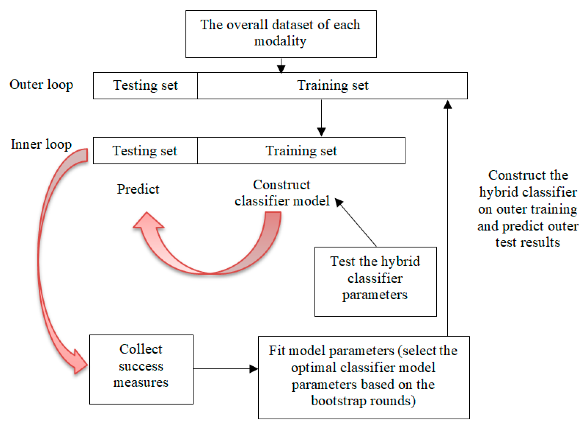
For each single modality, the accuracy of the hybrid classification algorithm is evaluated using the nested cross validation [61,62]. In this method, two nested CV loops are used to test the classifier, as shown in Figure 8. For the outer loop, the 1260 samples of each modality are split into seven folds. This means that in each fold we will have 210 testing samples and 1050 training samples. Every 210 samples are used as validation set (outer testing set), and the other 1050 samples are combined as outer training set. This procedure is repeated for each fold. Then, each outer training set is split into seven folds. Therefore, each fold will have 175 testing samples and 875 training samples.
A single set of 175 samples is accordingly used for validation (inner testing set), and the 875 samples are used as inner training set. This is implemented repeatedly for each fold. In this manner, the inner CV is used for selecting the best parameters that reduces the R M S E of our algorithm. For instance, the activation functions for the hidden and output layers, the learning rate, the maximum generations, the mutation ratio, the reproduction ratio, etc. The outer CV is used for final model testing.

4.3. First Experiment: Comparison of the Proposed FCM-GA-NN Model to the Developed F C M G A N N f i x e d

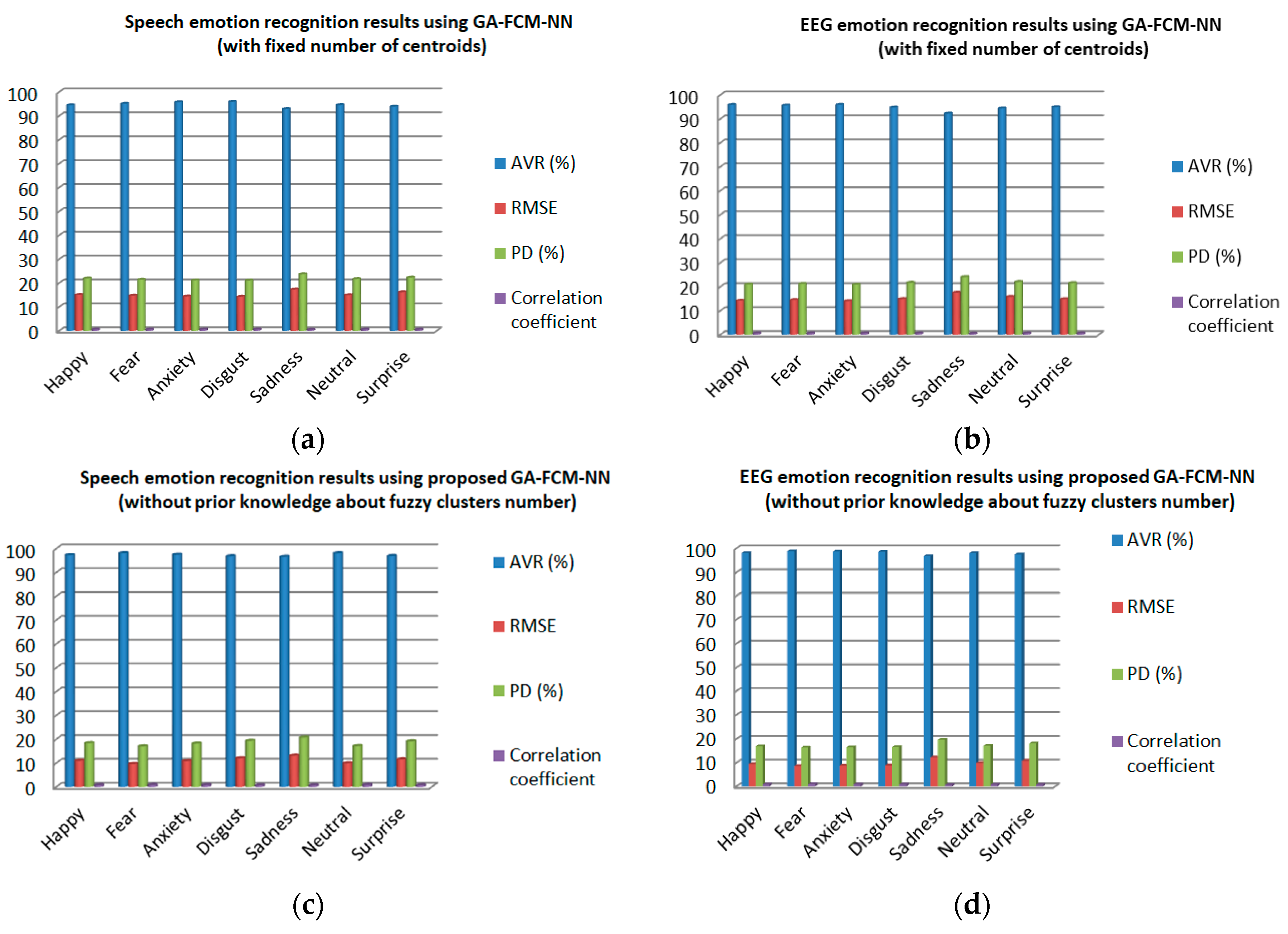
To reveal the efficiency of the proposed FCM-GA-NN model, it is crucial to compare it with another developed model that uses FCM and GA as hybrid to train NN [63]. The second model is centroid-based and requires previously a fixed cluster number. Contrarily, our model finds optimal fuzzy clusters with no prior knowledge on their number. Accordingly, the proposed model’s errors are compared with the second hybrid model. Figure 9 depicts the bar graph illustrations representing the AVR, R M S E s, P D s , and correlation coefficients ρ s among both measured and predicted values from the two models.
Taking fear class as an instance, the AVR rates of the proposed FCM-GA-NN model are 98.85% and 98.08% for EEG and speech modalities, respectively. By comparison, the AVRs using F C M G A N N f i x e d model are smaller than those of the proposed model, 95.66%, and 95.11% for EEG and speech modalities, respectively. The percent deviations ( P D s ) are 21.42% and 21.24% for speech and EEG modalities, respectively, which are also higher than the values from the proposed model. Furthermore, the proposed model exhibits ρ s of 0.9511 and 0.841, for EEG and speech modalities, respectively, which are higher than those obtained using the other model. The parameters that give the best accuracy for the two models are illustrated in Table 7.

4.4. Second Experiment: Speech Emotion Recognition

The second experiment depicted in Figure 10 was intended to investigate how robust the proposed hybrid fuzzy-evolutionary NN model is for speech emotion recognition. Accordingly, two databases for speakers of two different languages were used to test the model. The first dataset is collected during this study. The second dataset is a public one (SAVEE) [24]. For each dataset, the emotional features are extracted from the speech testing samples. Further, the proposed classifier is carried out.
The comparative results for the proposed model over the two speech datasets are illustrated as follows:
(a)
From Figure 9c, it can be vividly recognized that using the collected dataset, the proposed model achieved higher AVRs of 98.08%, 98.03%, 97.44%, 97.24%, 96.87%, 96.76%, and 96.55% for fear, neutral, anxiety, happy, surprise, disgust, and sadness classes, respectively. Likewise, it can be observed that during training the proposed model exhibits lower R M S E of 9.6233, 9.9299, 10.8219, 10.9501, 11.5206, 12.0312, and 13.1127, respectively, for the aforementioned classes. The model also gives lower P D s of 16.99%, 17.15%, 18.19%, 18.35%, 19.13%, 19.32%, and 20.67%, respectively, for the same classes.
(b)
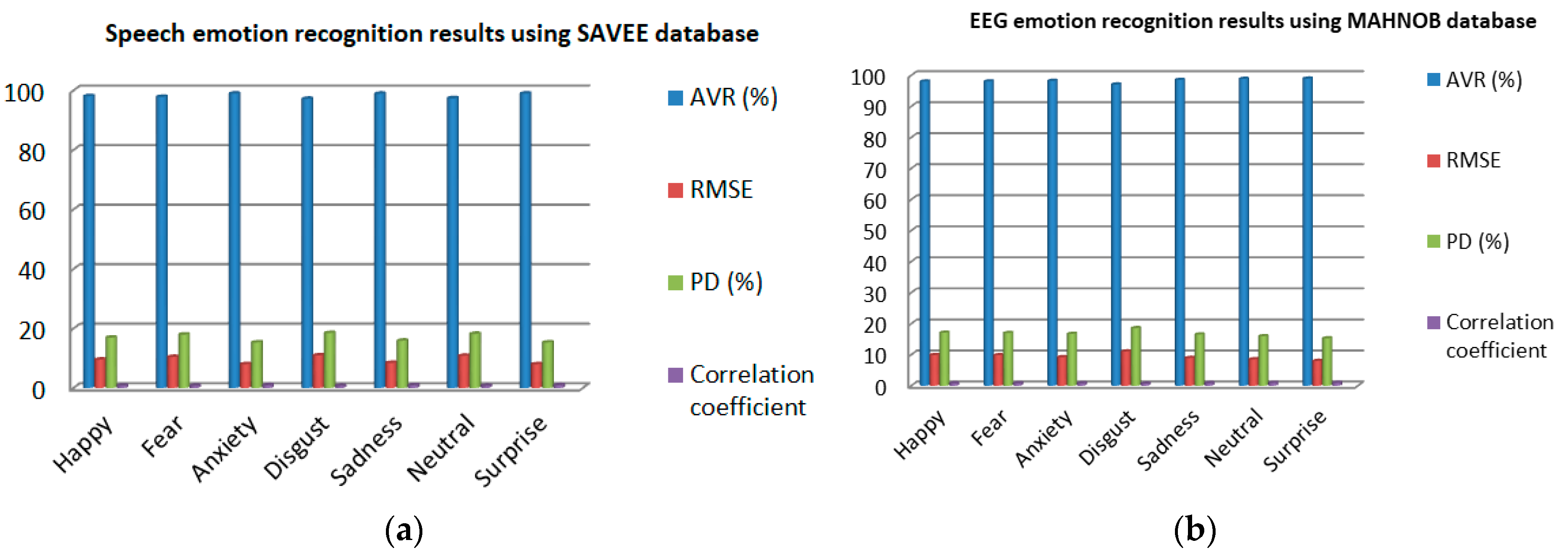
From Figure 11a, the proposed model achieved higher AVRs using the SAVEE dataset, 98.98%, 98.96%, 98.93%, 98.11%, 97.83%, 97.42%, and 97.21% for surprise, anxiety, sadness, happy, fear, neutral, and disgust classes, respectively. The minimum and maximum P D s occur at surprise class (15.31%) and disgust class (18.49%), respectively. The highest correlation coefficient ρ equals 0.9801, which is found at surprise class, while the lowest value is 0.733 and noted at disgust class.
By comparison, it is observed that the estimated measures give superior results over the two datasets. These results reflect the robustness of the mixing speech feature set in combination with the proposed hybrid model. On the other hand, there are low noticeable differences with respect to AVRs, R M S E s, P D s , and ρ s, obtained on emotion classes of the two datasets, for the favor of the SAVEE dataset. These differences may be due to the difference in the stimuli mode used to induce emotions. Whereas our speech dataset was acquired using music stimuli, the SAVEE dataset was collected using video stimuli.
Eventually, we compared our results to the other published results obtained using the public database of SAVEE, as illustrated in Table 8 [24,64,65]. It is obvious that our model yields superior results which outperform the state-of-the-art on speech emotion recognition, in terms of classification accuracy, where the total AVR achieved was 98.21%. This result supports the previously published works that have reported the powerful of the hybrid classification approaches in optimizing the speech recognition results in general [66,67].

4.5. Third Experiment: EEG Emotion Recognition

In terms of performance comparison purposes, we used two different datasets to check the robustness of the proposed model regarding EEG emotion recognition. The first dataset was collected during current research, which contains EEG signals of only 14 channels. The second dataset is a public one (MAHNOB) [45], which comprises EEG signals of 32 channels. MAHNOB dataset comprises user response recordings to a multimedia content. Video fragments from online sources, which last among 34.9 s and 117 s, using different content, were chosen for inducing nine emotions in the participants.
Next to each video clip, the subjects were asked to express their emotional status by a keyword like neutral, amusement, surprise, happiness, anger, disgust, sadness, fear, and anxiety. For each dataset, we estimated a set of extracted features from three domains, frequency, time, and time–frequency. Thereafter, the proposed model is applied to classify each dataset into seven-class emotions of EEG signals as depicted in Figure 12. The overall comparative results for the proposed model over the two datasets are overviewed as:
Using the collected dataset, the proposed model achieved higher AVRs of 98.85%, 98.69%, and 98.57%, respectively, for fear, anxiety, and disgust classes. It also gives lower R M S E s of 8.7233, 8.9111, and 8.9555, respectively for these classes, as shown in Figure 9d. The lowest and highest P D s found at fear class (16.33%) and sadness class (19.72%), respectively. The greatest ρ is 0.9511, also found at fear class.
With respect to the MAHNOB dataset, the proposed model gives higher AVRs of 98.96%, 98.91%, and 98.55%, respectively, for surprise, neutral, and sadness classes. On contrast, it gives lower R M S E s of 8.0112, 8.5402, and 8.9555, respectively, for the aforesaid classes, as shown in Figure 11b.
In terms of performance comparisons over the two datasets, the overall AVR of the proposed classifier is 98.26%, which shows low noticeable differences on the emotion classes for the favor of MAHNOB database. This can be interpreted by the differences in stimuli mode employed to induce emotions, where MAHNOB database uses visual stimuli. From these results, we deduce that the selected EEG feature set in combination to the proposed FCM-GA-NN model is robust for classifying emotions from EEG signals. We also conducted a comparison of the impact of fixed/sliding windowing methods on AVRs over the two datasets. As demonstrated in Table 9, the comparison reveals that fixed windowing returns better AVRs over the two compared datasets. The window size of 6 S was found to give the best AVR. We also compared our results to the other state-of-the-art results obtained using MAHNOB database, as shown in Table 10 [68,69,70]. The results indicate that the proposed model outperforms the state-of-the-art concerning EEG emotion recognition.

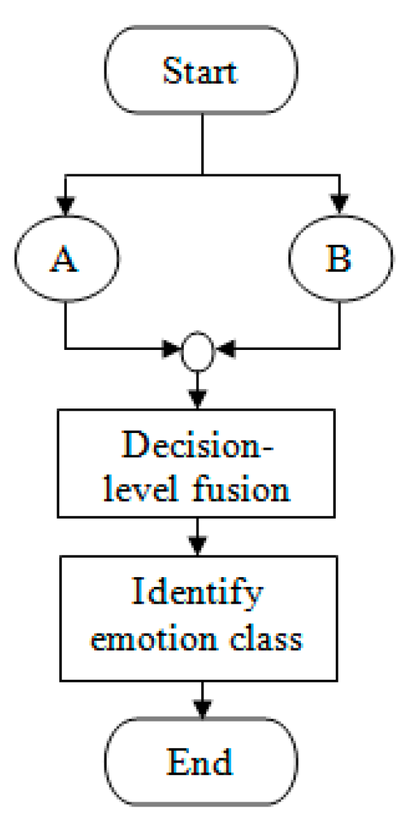
4.6. Fourth Experiment: Multi-Modal Emotion Recognition

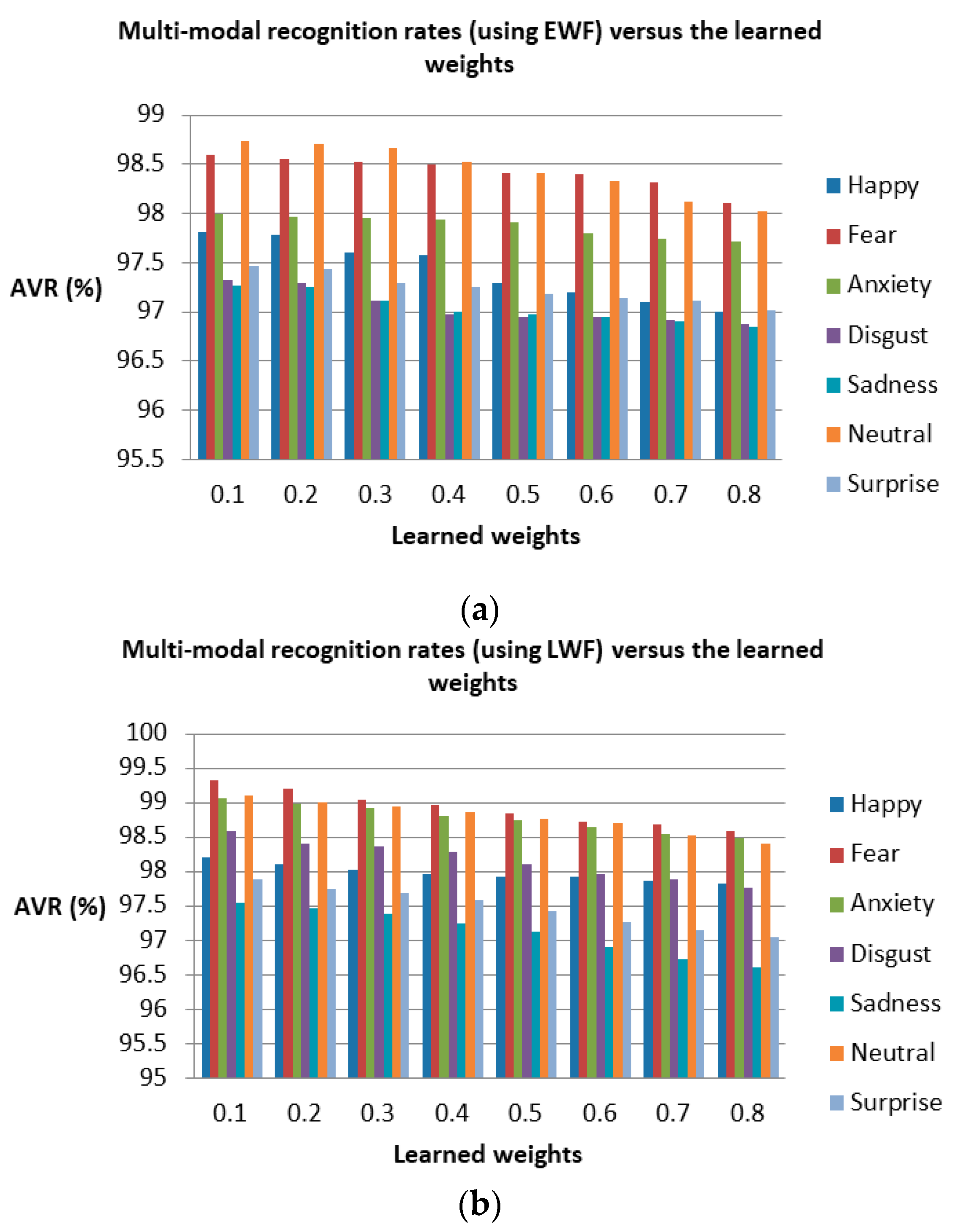
The experiment is depicted in Figure 13. Figure 14 depicts comparisons of the multi-modal emotion recognition results obtained using the two decision level algorithms i.e., EWF and LWF, when changing the value of the NN weight. From the figure, LWF outperforms the EWF over all cases of changing the learned NN weight. This recommends that predicting or approximating a weighting among the modalities performs better than classifying the samples employing individual modality outputs just as features.
Although the results taken by speech modality are only lower than those obtained with EEG only, this recommends that it is imperative to fuse speech and EEG signals, because there are emotional states that are recognized in a superior way from EEG than from speech. Eventually, the overall performance of multi-modal emotion aware system is 98.53%, which is higher in comparison to performance taken by our superior unimodal system, which is based upon EEG. Thus, the decision-level fusion is superior than the sole measurement.
In conclusion, consideration of multiple modalities is useful during the time that some modality features are lost or unreliable. This might happen, for instance, when the process of feature detection is critical due to noisy environmental factors, when corrupting the signals through transmission, or, if the system is incapable of recording one of the modalities. Therefore, the emotion recognition system must be robust enough to manage these real-life naturalistic scenarios.

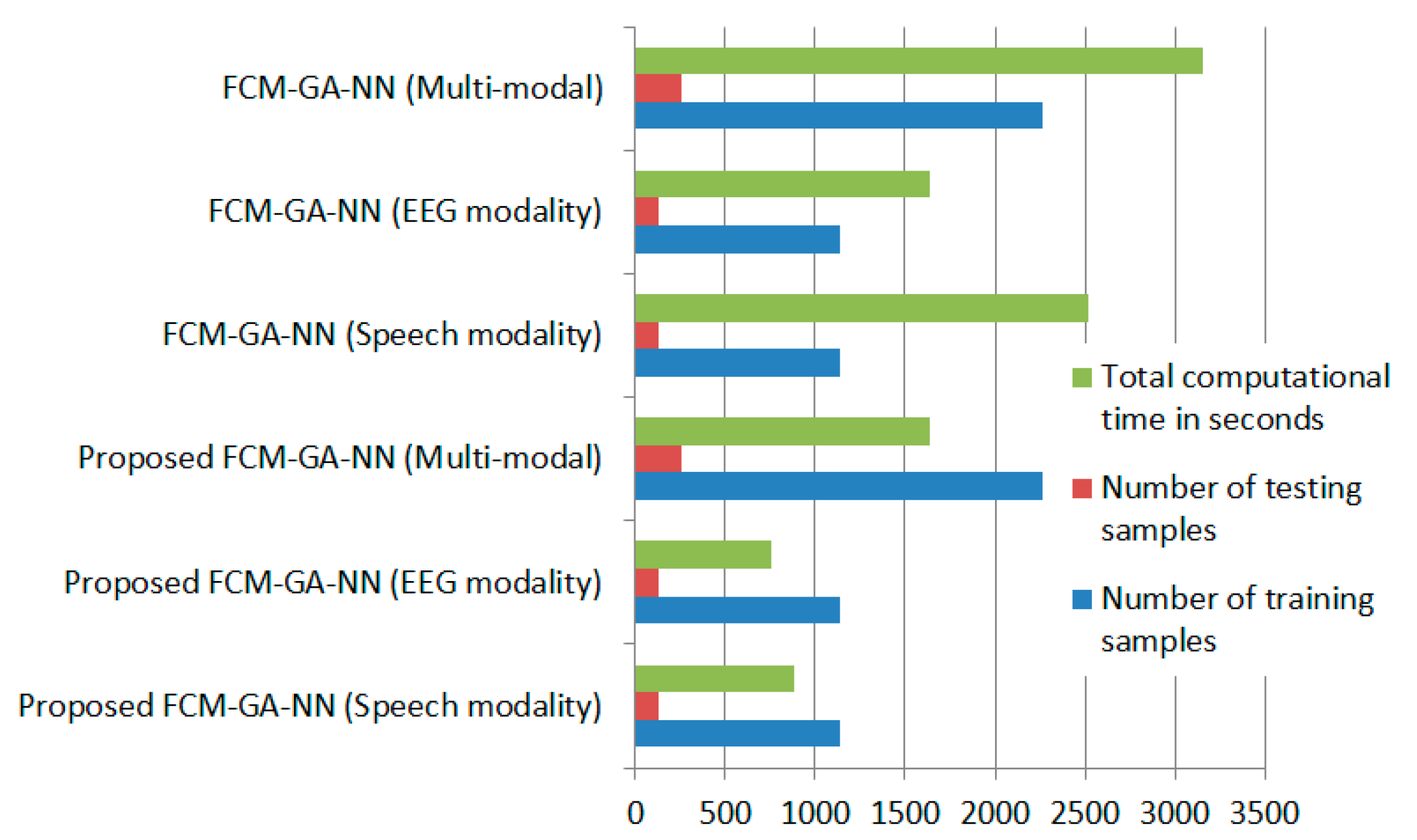
4.7. Computational Time Comparisons

The total run time (in seconds) is computed over our corpus for the three modalities, by testing the two algorithms, i.e., proposed FCM-GA-NN and F C M G A N N f i x e d . In terms of computational run time, Figure 15 depicts the comparative performance analysis of the two classifiers, during the CV. In comparison to the proposed FCM-GA-NN model, we can find that multi-modal emotion recognition using F C M G A N N f i x e d model reaches the highest total computational time of 3150 s. On contrary, the total computational time achieved by the proposed FCM-GA-NN model is reduced by about 1512 s.
.

5. Conclusions and Future Work

This paper introduces a novel multi-modal emotion recognition framework by fusing speech and EEG information. The EEG signals were utilized as internal channel complementing of speech for more reliable emotions recognition. For classification of unimodal data (speech and EEG) and multi-modal data, a proposed hybrid FCM-GA-NN soft computing model was introduced. The fitness function of the algorithm checks the optimal number of fuzzy clusters that reduces the classification error. The proposed model was compared to another developed FCM-GA-NN model that relies on determination of a fixed number for fuzzy clusters, and the fitness function of the algorithm checks the optimal chromosome that reduces the classification error. Accordingly, the proposed model’s errors were compared with the second model. The overall evaluation results of the two model, on emotion classes show the superiority of the proposed model. The algorithm was also implemented on two public databases for speech and EEG signals, namely SAVEE and MAHNOB, respectively. The overall performance of the proposed model reached 98.26%, 98.21%, and (98.06% and 97.28%) respectively for MAHNOB, SAVEE, and our dataset of its two modalities (EEG and speech, respectively). These results outperform the state-of-the-art results obtained using SAVEE and MAHNOB databases. Although the results taken by speech modality only (97.28%) are lower than those obtained with EEG only (98.06%), when applied to our dataset, this recommends fusing speech and EEG signals, because there are emotional states that are better recognized by the EEG than by speech. Therefore, after executing the automatic classification of every modality, the two modalities were fused on the decision-level. The comparative results of the fusion methods demonstrate that LWF performs better than EWF. By fusing speech and EEG modalities, the total computational time achieved by the proposed model also was reduced by about 1512 seconds than the F C M G A N N f i x e d model (with fixed number of centroids), when applied on our collected database. For the future work, we intend to recognize emotions through using a deep learning approach, which is optimized by the bio-inspired algorithms.

Author Contributions

Conceptualization, R.M.G. and A.D.A.; formal analysis, R.M.G. and A.D.A.; method and algorithms, R.M.G.; validation, R.M.G. and A.D.A.; visualization, R.M.G. and and A.D.A.; project management, R.M.G. and A.D.A.; writing—original draft: R.M.G.; writing—review and editing; R.M.G. and K.S.; supervision and paper revision, K.S.

Funding

This research received no external funding.

Conflicts of Interest

The authors declare no conflict of interest.

Appendix A. Algorithms

The pseudo-code of algorithms used in this paper is shown in Appendix A.
Algorithm A1: The proposed FCM-GA-NN model for emotion classification.
Inputs: (A) Parent population of each single modality M p (speech and EEG), indicated as P ( M p ) , ( p = 1 , 2 ) .
Output: Offspring population P t + 1 ( M p ) where each offspring contains an optimal fuzzy cluster set that minimizes the classification error.
  • For   each   sin gle   modality   M p ( p = 1 , 2 ) do
  •    Generate fuzzy memberships of each training sample from M p by one-step FCM clustering of Algorithm A2.
  •    Construct coded chromosome contain clusters centroids.
  •    Evaluate the fitness by Equations (11)–(17).
  •    Implement binary tournament selection on modality’s population P ( M p ) to get the mating pool P ( M p ) .
  •    For each p 1 to p s i z e
  •       Decode two chromosomes from P ( M p ) as matrices C p and C p + 1 using Equation (10).
  •       Compute fuzzy centroid sets F p and F p + 1 for C p and C p + 1 , respectively.
  •       For k = 1 to K // k indicates the index of k t h centroid of the chromosome
  •          Apply crossover on F p ( k ) and F p + 1 ( k ) according to Algorithm A3 to get F p ( k ) and F p + 1 ( k ) .
  •          Apply mutation on offsprings F p ( k ) and F p + 1 ( k ) according to Algorithm A4 to get F p ( k ) and F p + 1 ( k ) that represent updated centroid sets N p and N p + 1 .
  •       End For
  •    End For
  •    // Assigning object to a cluster
  •    For j = 1 to Z
  •       Compute distances among objects and every cluster centroid in N j , then update fuzzy memberships of U j by Equation (8) of Algorithm A2.
  •       Calculate the clustering indices by the maximum fuzzy memberships with regard to different clusters.
          IF empty cluster is found THEN
  •          Remove this empty cluster and then Go To Step 16.
  •       ELSE
  •          Assign fitness by Equations (11)–(17).
  •       END
  •        Get the resulting i-th offspring chromosome with its updated U j and objectives.
  •       End For
  •       Apply Algorithm A5 to the resulting population P t + 1 ( M p ) to compute the final solutions by clustering ensemble.
  •       Train the NN with solutions having the optimal cluster set that minimizes the classification error.
  • End For
Algorithm A2: The clustering algorithm.
  • Determine the cluster number u .
  • Set the initial value of μ i , k m at time m = 0 satisfying:
  • i = 1 u μ i , k m = 1 , k = 1 , 2 , , K ,          (5)
  • 0 < k = 1 K μ i , k m < K , i = 1 , 2 , , u , where:    (6)
    { I f k = 1 K μ i , k m = 0 , e m p t y   c l u s t e r I f k = 1 K μ i , k m = K , f e a t u r e v e c t o r   b e l o n g s   t o   i
  • Assume that K a m indicates the cluster index at time m and its initial value at m = 0 as 0 .
  • Set the centroid of a cluster i at time m as R i m then compute the u cluster centroids for the partition as: R i m = k = 1 K ( μ i , k m ) a x k k = 1 K ( μ i , k m ) a , i = 1 , , u , 1 < a .      (7)
  • Update membership degree for each emotion vector x k :
    μ i , k m + 1 = [ h = 1 u ( | | x k R i m | | 2 / | | x k R h m | | 2 ) 1 a 1 ] 1 (8)
  • Calculate the clustering index
  • K a m + 1 = k = 1 K i = 1 u [ ( μ i , k m + 1 ) a | | x k R i | | 2 ] ,    (9)
  • IF | K a m + 1 K a m | ε THEN
  • m = m + 1
  • Go to Step 7
  • END
Algorithm A3: Crossover algorithm.
Inputs: Parents F p and F p + 1 assigned as R , and M , respectively, where R = { r 1 , r 2 , r 3 , r 4 } , and M = { m 1 , m 2 , m 3 , m 4 }
Output: Children D 1 , and D 2
  • For i = 1 to y
  •   IF R a n d o m ( 0 , 1 ) < = 0.5 THEN
  •        C i = r i & O i = m i
  •        C R O S S ( C i , O i )
  •     Else
  •        C i = r i & O i = m i
  •   End IF
  • End For
  • C R O S S ( C , O )
  •  // random number between falls between 0 and 1
  •   g = R a n d o m ( 0 , 1 )
  •   IF g < = 0.5 THEN
  •        b e t a = ( 2 g ) 1 / ( e t a k + 1 )
  •     Else
  •        b e t a = ( 1 / ( 2 ( 1 g ) ) ) 1 / ( e t a k + 1 )
  •   End IF
  •   For j = 1 to x // x is the maximum dimension
  •     IF C j < O j THEN
  •        Q 1 = C j & Q 2 = O j
  •     Else
  •        Q 1 = O j & Q 2 = C j
  •     End IF
  •      D j 1 = [ ( 1 + b e t a ) Q 1 + ( 1 b e t a ) Q 2 ] 2 (19)
  •      D j 2 = [ ( 1 b e t a ) Q 1 + ( 1 + b e t a ) Q 2 ] 2 (20)
  •     End For
  •     IF R a n d o m ( 0 , 1 ) < = 0.5 THEN
  •        C = D 1 & O = D 2
  •       Else
  •         C = D 2 & O = D 1
  •   End IF
  • Return D 1 , and D 2
Algorithm A4:  Mutation algorithm.
Inputs: Set of crossover-subjected chromosomes C R , C R = { c r 1 , c r 2 , c r 3 , , c r K }
Output: mutated chromosomes
  • // k is the index of k t h centroid of the chromosome
  • For k = 1 to K
  •   For j = 1 to J // j is the index of chromosome point
  •    Generate a random number from 0 to : B = r a n d o m ( 0 , 1 )
  •    IF B P T
  •     Generate z j random number f 1 , f 2 , , f j , z from [ 0 , 1 ] for the j t h point of the centroid E k , j k
  •     Replace E k , j k by f k / k = 1 z j f k
  •    End IF
  •   End For
  • End For
Algorithm A5: Final solution computation by clustering ensemble.
Inputs: Solutions set T = { s 1 , s 2 , , s n } indicating fuzzy memberships.
Output: Final cluster label S * .
  • For j = 1 to V // for each solution>
  •   Calculate the ranking vectors R ( s j ) .
  •   Calculate the aggregated ranks based upon the sum of each solution to get a vector: R ˜ t = [ R j ( 1 ) , . R j ( 2 ) , . . , R j ( n ) ] .
    End For
  • Sort T by the aggregated ranks (values of R ) in ascending order and obtain a new solutions set:
    T = { s 1 , s 2 , , s n } .
  • Assume an ensemble of Z size.
  • Select the first Z solutions to get a subset of non-dominated solutions: T n e w = { s 1 , s 2 , , s Z }
  • For j = 1 to Z // for each non-dominated solution s j in T n e w
  •   Decode s j by Equation (10).
  •   Assign every object k of s j to a cluster i by the maximum of μ i , k m , where 1 k K .
  •   Get a vector x j containing n cluster labels.
  •   Considering the size of T n e w is Z , add the resulting vector x j to a matrix E of size Z × n .
  • End
  • Apply the clustering ensemble algorithm to the resulting matrix E , where each row represents one clustering solution.
  • Return a vector S * comprising n cluster labels as the final output.

References

  1. Kolodyazhniy, V.; Kreibig, S.D.; Gross, J.J.; Roth, W.T.; Wilhelm, F.H. An affective computing approach to physiological emotion specificity: Toward subject-independent and stimulus-independent classification of film-induced emotions. Psychophysiology 2011, 48, 908–922. [Google Scholar] [CrossRef] [PubMed]
  2. Liu, Y.-J.; Yu, M.; Zhao, G.; Song, J.; Ge, Y.; Shi, Y. Real-Time Movie-Induced Discrete Emotion Recognition from EEG Signals. IEEE Trans. Affect. Comput. 2018, 9, 550–562. [Google Scholar] [CrossRef]
  3. Menezes, M.L.R.; Samara, A.; Galway, L.; Sant’Anna, A.; Verikas, A.; Alonso-Fernandez, F.; Wang, H.; Bond, R. Towards emotion recognition for virtual environments: an evaluation of EEG features on benchmark dataset. Pers. Ubiquitous Comput. 2017, 21, 1003–1013. [Google Scholar] [CrossRef]
  4. Gharavian, D.; Bejani, M.; Sheikhan, M. Audio-visual emotion recognition using FCBF feature selection method and particle swarm optimization for fuzzy ARTMAP neural networks. Multimed. Tools Appl. 2016, 76, 2331–2352. [Google Scholar] [CrossRef]
  5. Li, Y.; He, Q.; Zhao, Y.; Yao, H. Multi-modal Emotion Recognition Based on Speech and Image. Adv. Multimed. Inf. Process. – PCM 2017 Lecture Notes Comput. Sci. 2018, 844–853. [Google Scholar]
  6. Rahdari, F.; Rashedi, E.; Eftekhari, M. A Multimodal Emotion Recognition System Using Facial Landmark Analysis. Iran. J. Sci. Tech. Trans. Electr. Eng. 2018, 43, 171–189. [Google Scholar] [CrossRef]
  7. Wan, P.; Wu, C.; Lin, Y.; Ma, X. Optimal Threshold Determination for Discriminating Driving Anger Intensity Based on EEG Wavelet Features and ROC Curve Analysis. Information 2016, 7, 52. [Google Scholar] [CrossRef]
  8. Poh, N.; Bengio, S. How do correlation and variance of base-experts affect fusion in biometric authentication tasks? IEEE Trans. Signal Process. 2005, 53, 4384–4396. [Google Scholar] [CrossRef] [Green Version]
  9. Majumder, N.; Hazarika, D.; Gelbukh, A.; Cambria, E.; Poria, S. Multimodal sentiment analysis using hierarchical fusion with context modeling. Knowl.-Based Syst. 2018, 161, 124–133. [Google Scholar] [CrossRef] [Green Version]
  10. Adeel, A.; Gogate, M.; Hussain, A. Contextual Audio-Visual Switching For Speech Enhancement in Real-World Environments. Inf. Fusion 2019. [Google Scholar]
  11. Gogate, M.; Adeel, A.; Marxer, R.; Barker, J.; Hussain, A. DNN Driven Speaker Independent Audio-Visual Mask Estimation for Speech Separation. In Proceedings of the Interspeech 2018, Hyderabad, India, 2–6 September 2018. [Google Scholar]
  12. Huang, F.; Zhang, X.; Zhao, Z.; Xu, J.; Li, Z. Image–text sentiment analysis via deep multimodal attentive fusion. Knowl.-Based Syst. 2019, 167, 26–37. [Google Scholar] [CrossRef]
  13. Ahmadi, E.; Jasemi, M.; Monplaisir, L.; Nabavi, M.A.; Mahmoodi, A.; Jam, P.A. New efficient hybrid candlestick technical analysis model for stock market timing on the basis of the Support Vector Machine and Heuristic Algorithms of Imperialist Competition and Genetic. Expert Syst. Appl. 2018, 94, 21–31. [Google Scholar] [CrossRef]
  14. Melin, P.; Miramontes, I.; Prado-Arechiga, G. A hybrid model based on modular neural networks and fuzzy systems for classification of blood pressure and hypertension risk diagnosis. Expert Syst. Appl. 2018, 107, 146–164. [Google Scholar] [CrossRef]
  15. Engberg, I.; Hansen, A. Documentation of the Danish emotional speech database des 1996. Available online: http://kom.aau.dk/~tb/speech/Emotions/des (accessed on 4 July 2019).
  16. Wang, K.; An, N.; Li, B.N. Speech emotion recognition using Fourier parameters. IEEE Trans. Affect. Comput. 2015, 6, 69–75. [Google Scholar] [CrossRef]
  17. Eyben, F.; Scherer, K.R.; Schuller, B.W.; Sundberg, J.; Andre, E.; Busso, C.; Devillers, L.Y.; Epps, J.; Laukka, P.; Narayanan, S.S.; et al. The Geneva Minimalistic Acoustic Parameter Set (GeMAPS) for Voice Research and Affective Computing. IEEE Trans. Affect. Comput. 2016, 7, 190–202. [Google Scholar] [CrossRef]
  18. Tahon, M.; Devillers, L. Towards a Small Set of Robust Acoustic Features for Emotion Recognition: Challenges. IEEE/ACM Transact. Audio Speech Lang. Process. 2016, 24, 16–28. [Google Scholar] [CrossRef]
  19. Zhao, J.; Mao, X.; Chen, L. Speech emotion recognition using deep 1D & 2D CNN LSTM networks. Biomed. Signal Process. Control 2019, 47, 312–323. [Google Scholar]
  20. Liu, Z.-T.; Wu, M.; Cao, W.-H.; Mao, J.-W.; Xu, J.-P.; Tan, G.-Z. Speech emotion recognition based on feature selection and extreme learning machine decision tree. Neurocomputing 2018, 273, 271–280. [Google Scholar] [CrossRef]
  21. Alonso, J.B.; Cabrera, J.; Medina, M.; Travieso, C.M. New approach in quantification of emotional intensity from the speech signal: Emotional temperature. Expert Syst. Appl. 2015, 42, 9554–9564. [Google Scholar] [CrossRef]
  22. Cao, H.; Verma, R.; Nenkova, A. Speaker-sensitive emotion recognition via ranking: Studies on acted and spontaneous speech. Comput. Speech Lang. 2015, 29, 186–202. [Google Scholar] [CrossRef] [PubMed]
  23. D Griol, D.; Molina, J.M.; Callejas, Z. Combining speech-based and linguistic classifiers to recognize emotion in user spoken utterances. Neurocomputing 2019, 326-327, 132–140. [Google Scholar] [CrossRef]
  24. Yogesh, C.K.; Hariharan, M.; Ngadiran, R.; Adom, A.; Yaacob, S.; Polat, K. Hybrid BBO_PSO and higher order spectral features for emotion and stress recognition from natural speech. Appl. Soft Comput. 2017, 56, 217–232. [Google Scholar]
  25. Shon, D.; Im, K.; Park, J.-H.; Lim, D.-S.; Jang, B.; Kim, J.-M. Emotional Stress State Detection Using Genetic Algorithm-Based Feature Selection on EEG Signals. Int. J. Environ. Res. Public Health 2018, 15, 2461. [Google Scholar] [CrossRef] [PubMed]
  26. Mert, A.; Akan, A. Emotion recognition based on time–frequency distribution of EEG signals using multivariate synchrosqueezing transform. Digit. Signal Process. 2018, 81, 106–115. [Google Scholar] [CrossRef]
  27. Zoubi, O.A.; Awad, M.; Kasabov, N.K. Anytime multipurpose emotion recognition from EEG data using a Liquid State Machine based framework. Artif. Intell. Med. 2018, 86, 1–8. [Google Scholar] [CrossRef] [PubMed]
  28. Zhang, Y.; Ji, X.; Zhang, S. An approach to EEG-based emotion recognition using combined feature extraction method. Neurosc. Lett. 2016, 633, 152–157. [Google Scholar] [CrossRef] [PubMed]
  29. Bhatti, A.M.; Majid, M.; Anwar, S.M.; Khan, B. Human emotion recognition and analysis in response to audio music using brain signals. Comput. Human Behav. 2016, 65, 267–275. [Google Scholar] [CrossRef]
  30. Ma, Y.; Hao, Y.; Chen, M.; Chen, J.; Lu, P.; Košir, A. Audio-visual emotion fusion (AVEF): A deep efficient weighted approach. Inf. Fusion 2019, 46, 184–192. [Google Scholar] [CrossRef]
  31. Hossain, M.S.; Muhammad, G. Emotion recognition using deep learning approach from audio–visual emotional big data. Inf. Fusion 2019, 49, 69–78. [Google Scholar] [CrossRef]
  32. Huang, Y.; Yang, J.; Liao, P.; Pan, J. Fusion of Facial Expressions and EEG for Multimodal Emotion Recognition. Comput. Intell. Neurosci. 2017, 2017, 1–8. [Google Scholar] [CrossRef] [Green Version]
  33. Abhang, P.A.; Gawali1, B.W. Correlation of EEG Images and Speech Signals for Emotion Analysis. Br. J. Appl. Sci. Tech. 2015, 10, 1–13. [Google Scholar] [CrossRef]
  34. MacQueen, J.B. Some methods for classification and analysis of multivariate observations. In Proceedings of the Fifth Berkeley Symposium on Mathematical Statistics and Probability, Berkeley, CA, USA, 21 June–18 July 1965 and 27 December 1965–7 January 1966; pp. 281–297. [Google Scholar]
  35. Bezdek, J. Corrections for “FCM: The fuzzy c-means clustering algorithm”. Comput. Geosci. 1985, 11, 660. [Google Scholar] [CrossRef]
  36. Duda, R.O.; Hart, P.E.; Stork, D.G. Pattern Classification, 2nd ed.; Wiley: Hoboken, NJ, USA, 2001. [Google Scholar]
  37. Ripon, K.; Tsang, C.-H.; Kwong, S. Multi-Objective Data Clustering using Variable-Length Real Jumping Genes Genetic Algorithm and Local Search Method. In Proceedings of the 2006 IEEE International Joint Conference on Neural Network, Vancouver, BC, Canada, 16–21 July 2006. [Google Scholar]
  38. Karaboga, D.; Ozturk, C. A novel clustering approach: Artificial Bee Colony (ABC) algorithm. Appl. Soft Comput. 2011, 11, 652–657. [Google Scholar] [CrossRef]
  39. Zabihi, F.; Nasiri, B. A Novel History-driven Artificial Bee Colony Algorithm for Data Clustering. Appl. Soft Comput. 2018, 71, 226–241. [Google Scholar] [CrossRef]
  40. Islam, M.Z.; Estivill-Castro, V.; Rahman, M.A.; Bossomaier, T. Combining K-Means and a genetic algorithm through a novel arrangement of genetic operators for high quality clustering. Expert Syst. Appl. 2018, 91, 402–417. [Google Scholar] [CrossRef]
  41. Song, R.; Zhang, X.; Zhou, C.; Liu, J.; He, J. Predicting TEC in China based on the neural networks optimized by genetic algorithm. Adv. Space Res. 2018, 62, 745–759. [Google Scholar] [CrossRef]
  42. Krzywanski, J.; Fan, H.; Feng, Y.; Shaikh, A.R.; Fang, M.; Wang, Q. Genetic algorithms and neural networks in optimization of sorbent enhanced H2 production in FB and CFB gasifiers. Energy Convers. Manag. 2018, 171, 1651–1661. [Google Scholar] [CrossRef]
  43. Vakili, M.; Khosrojerdi, S.; Aghajannezhad, P.; Yahyaei, M. A hybrid artificial neural network-genetic algorithm modeling approach for viscosity estimation of graphene nanoplatelets nanofluid using experimental data. Int. Commun. Heat Mass Transf. 2017, 82, 40–48. [Google Scholar]
  44. Sun, W.; Xu, Y. Financial security evaluation of the electric power industry in China based on a back propagation neural network optimized by genetic algorithm. Energy 2016, 101, 366–379. [Google Scholar] [CrossRef]
  45. Soleymani, M.; Lichtenauer, J.; Pun, T.; Pantic, M. A Multimodal Database for Affect Recognition and Implicit Tagging. IEEE Trans. Affect. Comput. 2012, 3, 42–55. [Google Scholar] [CrossRef]
  46. Harley, J.M.; Bouchet, F.; Hussain, M.S.; Azevedo, R.; Calvo, R. A multi-componential analysis of emotions during complex learning with an intelligent multi-agent system. Comput. Human Behav. 2015, 48, 615–625. [Google Scholar] [CrossRef]
  47. Ozdas, A.; Shiavi, R.; Silverman, S.; Silverman, M.; Wilkes, D. Investigation of Vocal Jitter and Glottal Flow Spectrum as Possible Cues for Depression and Near-Term Suicidal Risk. IEEE Trans. Biomed. Eng. 2004, 51, 1530–1540. [Google Scholar] [CrossRef] [PubMed]
  48. Muthusamy, H.; Polat, K.; Yaacob, S. Particle Swarm Optimization Based Feature Enhancement and Feature Selection for Improved Emotion Recognition in Speech and Glottal Signals. PLoS ONE 2015, 10, e0120344. [Google Scholar] [CrossRef] [PubMed]
  49. Jebelli, H.; Hwang, S.; Lee, S. EEG Signal-Processing Framework to Obtain High-Quality Brain Waves from an Off-the-Shelf Wearable EEG Device. J. Comput. Civil Eng. 2018, 32, 04017070. [Google Scholar] [CrossRef]
  50. Ferree, T.C.; Luu, P.; Russell, G.S.; Tucker, D.M. Scalp electrode impedance, infection risk, and EEG data quality. Clin. Neurophys. 2001, 112, 536–544. [Google Scholar] [CrossRef]
  51. Delorme, A.; Makeig, S. EEGLAB: An open source toolbox for analysis of single-trial EEG dynamics including independent component analysis. J. Neurosci. Methods 2004, 134, 9–21. [Google Scholar] [CrossRef] [PubMed]
  52. Ayadi, M.E.; Kamel, M.S.; Karray, F. Survey on speech emotion recognition: Features, classification schemes, and databases. Pattern Recogn. 2011, 44, 572–587. [Google Scholar] [CrossRef]
  53. Candra, H.; Yuwono, M.; Chai, R.; Handojoseno, A.; Elamvazuthi, I.; Nguyen, H.T.; Su, S. Investigation of window size in classification of EEG-emotion signal with wavelet entropy and support vector machine. In Proceedings of the 37th Annual International Conference of the IEEE Engineering in Medicine and Biology Society (EMBC), Milano, Italy, 25–29 August 2015. [Google Scholar]
  54. Ou, G.; Murphey, Y.L. Multi-class pattern classification using neural networks. Pattern Recogn. 2007, 40, 4–18. [Google Scholar] [CrossRef]
  55. Yang, J.; Yang, X.; Zhang, J. A Parallel Multi-Class Classification Support Vector Machine Based on Sequential Minimal Optimization. In Proceedings of the First International Multi-Symposiums on Computer and Computational Sciences (IMSCCS06), Hangzhou, China, 20–24 June 2006. [Google Scholar]
  56. Ghoniem, R.M.; Shaalan, K. FCSR - Fuzzy Continuous Speech Recognition Approach for Identifying Laryngeal Pathologies Using New Weighted Spectrum Features. In Proceedings of the 2017 International Conference on Advanced Intelligent Systems and Informatics (AISI), Cairo, Egypt, 9–11 September 2017; pp. 384–395. [Google Scholar]
  57. Tan, J.H. On Cluster Validity for Fuzzy Clustering. Master Thesis, Applied Mathematics Department, Chung Yuan Christian University, Taoyuan, Taiwan, 2000. [Google Scholar]
  58. Wikaisuksakul, S. A multi-objective genetic algorithm with fuzzy c-means for automatic data clustering. Appl. Soft Comput. 2014, 24, 679–691. [Google Scholar] [CrossRef]
  59. Strehl, A.; Ghosh, J. Cluster ensembles—a knowledge reuse framework for combining multiple partitions. J. Mach. Learn. Res. 2002, 3, 583–617. [Google Scholar]
  60. Koelstra, S.; Patras, I. Fusion of facial expressions and EEG for implicit affective tagging. Image Vision Comput. 2013, 31, 164–174. [Google Scholar] [CrossRef]
  61. Dora, L.; Agrawal, S.; Panda, R.; Abraham, A. Nested cross-validation based adaptive sparse representation algorithm and its application to pathological brain classification. Expert Syst. Appl. 2018, 114, 313–321. [Google Scholar] [CrossRef]
  62. Oppedal, K.; Eftestøl, T.; Engan, K.; Beyer, M.K.; Aarsland, D. Classifying Dementia Using Local Binary Patterns from Different Regions in Magnetic Resonance Images. Int. J. Biomed. Imaging 2015, 2015, 1–14. [Google Scholar] [CrossRef] [PubMed]
  63. Gao, X.; Lee, G.M. Moment-based rental prediction for bicycle-sharing transportation systems using a hybrid genetic algorithm and machine learning. Comput. Ind. Eng. 2019, 128, 60–69. [Google Scholar] [CrossRef]
  64. Liu, Z.-T.; Xie, Q.; Wu, M.; Cao, W.-H.; Mei, Y.; Mao, J.-W. Speech emotion recognition based on an improved brain emotion learning model. Neurocomputing 2018, 309, 145–156. [Google Scholar] [CrossRef]
  65. Özseven, T. A novel feature selection method for speech emotion recognition. Appl. Acoust. 2019, 146, 320–326. [Google Scholar] [CrossRef]
  66. Ghoniem, R.M. Deep Genetic Algorithm-Based Voice Pathology Diagnostic System. In Proceedings of the Natural Language Processing and Information Systems Lecture Notes in Computer Science, Salford, UK, 26–28 June 2019; pp. 220–233. [Google Scholar]
  67. Ghoniem, R.M.; Shaalan, K. A Novel Arabic Text-independent Speaker Verification System based on Fuzzy Hidden Markov Model. Procedia Comput. Sci. 2017, 117, 274–286. [Google Scholar] [CrossRef]
  68. Nakisa, B.; Rastgoo, M.N.; Tjondronegoro, D.; Chandran, V. Evolutionary computation algorithms for feature selection of EEG-based emotion recognition using mobile sensors. Expert Syst. Appl. 2018, 93, 143–155. [Google Scholar] [CrossRef] [Green Version]
  69. Munoz, R.; Olivares, R.; Taramasco, C.; Villarroel, R.; Soto, R.; Barcelos, T.S.; Merino, E.; Alonso-Sánchez, M.F. Using Black Hole Algorithm to Improve EEG-Based Emotion Recognition. Comput. Intell. Neurosci. 2018, 2018, 1–21. [Google Scholar] [CrossRef]
  70. Munoz, R.; Olivares, R.; Taramasco, C.; Villarroel, R.; Soto, R.; Alonso-Sánchez, M.F.; Merino, E.; Albuquerque, V.H.C.D. A new EEG software that supports emotion recognition by using an autonomous approach. Neural Comput. Appl. 2018. [Google Scholar] [CrossRef]
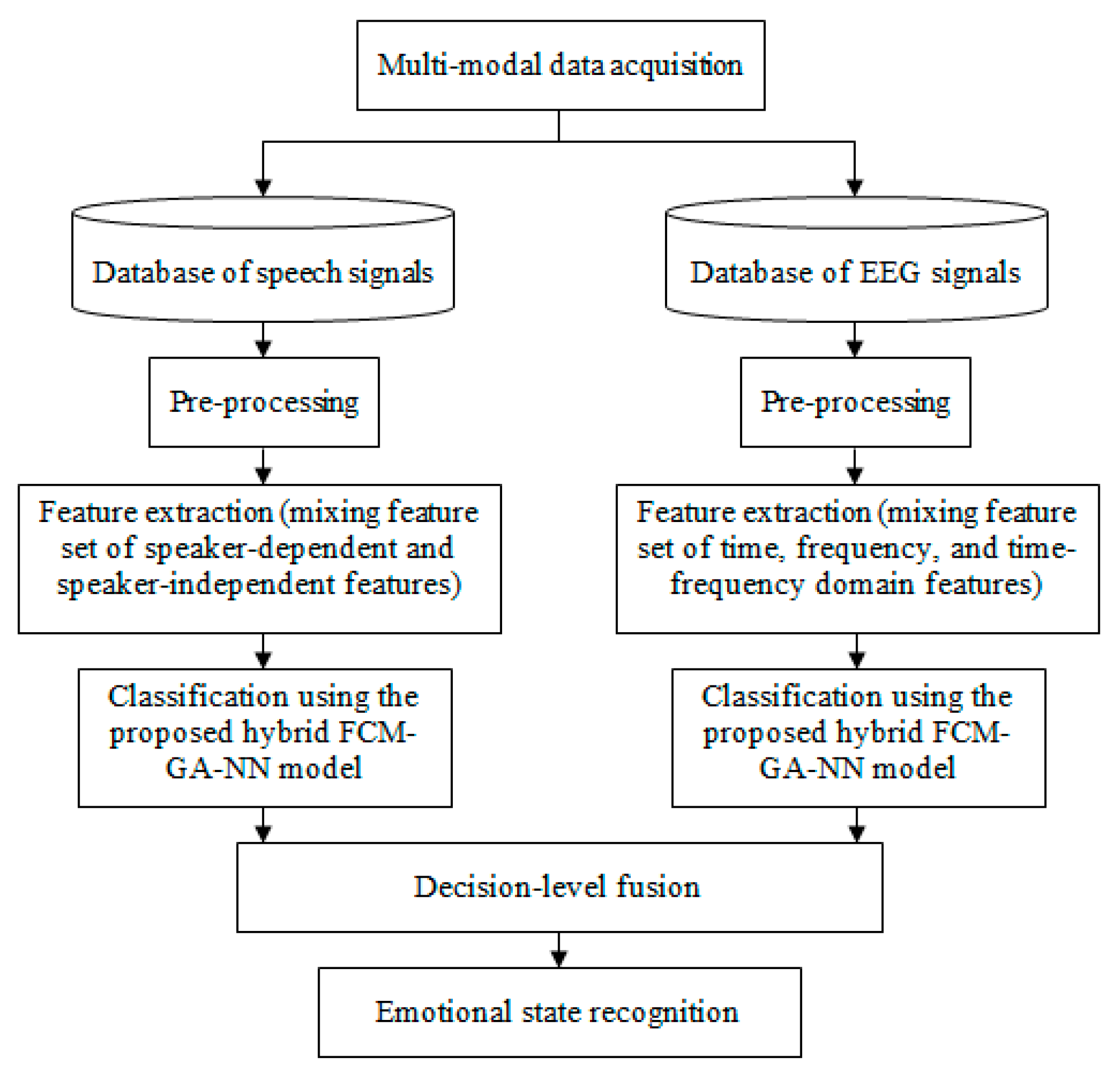
Figure 1. Architecture of the multi-modal emotion aware system.
Information 10 00239 g001
Figure 2. Structure of audio tracks that were played for participants: 5 s of silence, then 60 s from every track, and in between 15 s for performing emotion labelling.
Information 10 00239 g002
Figure 3. Emotiv-EPOC headset with 16-channel placement; 14-channels were intended to detect signals of human brain, along with 2 reference channels situated adjacent to the ears. Channel locations were based upon the 10/20 system of electrodes placement.
Information 10 00239 g003
Figure 4. Flowchart of the proposed hybrid FCM-GA-NN model for recognizing human emotions.
Information 10 00239 g004
Figure 5. Chromosome representation.
Information 10 00239 g005
Figure 6. Crossover procedure of two chromosomes in our framework.
Information 10 00239 g006
Figure 7. Clustering ensemble based final solution.
Information 10 00239 g007
Figure 8. Nested cross validation.
Information 10 00239 g008
Figure 9. The overall evaluation results for the proposed FCM-GA-NN model, and F C M G A N N f i x e d model, on different emotion classes of each single modality (speech and EEG).
Information 10 00239 g009
Figure 10. Cross validation of speech emotion recognition using the proposed FCM-GA-NN model.
Information 10 00239 g010
Figure 11. The overall evaluation results for the proposed FCM-GA-NN model over two publicly available databases: (a) SAVEE database for speech emotion recognition, and (b) MAHNOB for EEG emotion recognition.
Information 10 00239 g011
Figure 12. Cross validation of EEG emotion recognition using proposed model.
Information 10 00239 g012
Figure 13. Flowchart of multi-modal emotion recognition using speech and EEG information.
Information 10 00239 g013
Figure 14. Multi-modal emotion recognition results using (a) EWF and (b) LWF versus the learned weights.
Information 10 00239 g014
Figure 15. Computational time comparisons of the three modalities (speech, EEG, multi-modal), using the two algorithms i.e., the proposed FCM-GA-NN and F C M G A N N f i x e d .
Information 10 00239 g015
Table 1. Recent Research on speech emotion recognition.
ReferencePublication YearCorpusSpeech AnalysisFeature SelectionClassifierClassification Accuracy
[19]2019Berlin EmoDB The local feature learning blocks (LFLB) and the LSTM are used to learn the local and global features from the raw signals and log-mel spectrograms.-1D & 2D CNN LSTM networks.95.33% and 95.89% for speaker-dependent and speaker-independent results, respectively.
IEMOCAP89.16% and 52.14% for speaker-dependent and speaker-independent results, respectively.
[20]2018Chinese speech database from Chinese academy of sciences (CASIA)Speaker-dependent features, and speaker-independent features.A correlation analysis and Fisher-based method.Extreme learning machine (ELM)89.6%
[21]2015BESTwo prosodic features and four paralinguistic features of the pitch and spectral energy balance.NoneSupport vector machines (SVM)94.9%
LDC Emotional Prosody Speech and Transcripts 88.32%
Polish Emotional Speech Database90%
[22]2015BESSpectral and prosodic features.NoneRanking SVMs82.1%
LDC52.4%
FAU Aibo39.4%
Table 2. Recent research on electroencephalogram (EEG)-based emotion recognition.
ReferenceCorpusPublication YearFeature ExtractionFeature SelectionClassifierEmotion ClassesClassification Accuracy
[26]DEAP database2018Multivariate synchrosqueezing transform.Non-negative matrix factorization and independent component analysis.Artificial Neural Network (ANN)Arousal/valence states (high arousal-high valence, high arousal-low valence, low arousal-low valence, low arousal -high valence).82.03% and 82.11% for valence and arousal state recognition.
[27]DEAP database2018Liquid State Machines (LSM)-Decision TreesValence, arousal as well as liking classes.84.63%, 88.54%, and 87.03% for valence, arousal, and liking classes, respectively.
[28] DEAP database2016Empirical mode decomposition and sample entropy.NoneSVMArousal/valence states (high arousal-high valence, high arousal-low valence, low arousal-low valence, low arousal-high valence).94.98% for binary-class tasks, and 93.20% for the multi-class task.
[29]Collected database2016Features of time (i.e., Latency to Amplitude Ration, Peak to Peak Signal Value, etc.), frequency (i.e., Power Spectral Density, and Band Power), and wavelet domain.NoneThree different classifiers (ANN, k-nearest neighbor, and SVM)Happiness, sadness, love, and, anger78.11% for ANN classifier.
Table 3. Research on multi-modal emotion recognition utilizing multiple modalities.
ReferencePublication YearCorpusFused ModalitiesFeature ExtractionFusion ApproachClassifierClassification Accuracy
[30]2019RML, Enterface05, and BAUM-1sSpeech and image features2D convolutional neural network for audio signals, and 3D convolutional neural network for image features.Deep belief networkSVM85.69% for Enterface05 dataset in case of multi-modal classification based upon six discrete emotions.
91.3% and 91.8%, respectively, for binary arousal-valence model, in case of multi-modal classification using Enterface05 dataset.
[31]2019Private database, namely, Big Data and a publicly available database of Enterface05.Speech and videoFor speech feature extraction, Mel-spectrogram is obtained.
For video feature extraction, a number of representative frames are selected from a video segment.
Extreme Learning Machines (ELM)The CNN is separately fed with speech and video features, respectively.An accuracy of 99.9% and 86.4% for the favor of ELM fusion using the Big Data and Enterface05, respectively.
[32]2017MAHNOB-HCI databaseFacial expressions and EEGAs for facial expressions, the appearance features are estimated from each frame block then the expression percentage feature is computed.
The EEG features are calculated using the Welch’s Averaged Periodogram.
Feature-level fusion by concatenating all features within a single vector, in addition to decision-level fusion by processing each modality in a separate way, and amalgamating results from their special classifiers in the recognition stage.For decision-level fusion, LWF and EWF are used.
For feature-level fusion, the paper used several statistical fusion methods like Canonical Correlation Analysis (CCA) and Multiple Feature Concatenation (MFC).
For decision-level fusion, LWF achieved recognition rates of 66.28% and 63.22%, for valence and arousal classes, respectively.
For feature-level fusion, MFC achieved recognition rates of 57.47% and 58.62%, for valence and arousal classes, respectively.
[33]2015Private database, which were collected from university students.EEG images along with speech signalsFor EEG images, the features were extracted using the threshold, the Sobel edge detection, and some statistical measures (e.g., mean, variance, standard deviation, etc.). While the intensity, the RMS Energy, and the pitch were used for speech signal feature extraction.None (the study investigated correlation of EEG images as well as Speech signals)NoneThe significance accuracy of correlation coefficient was about 95% for the favor of said emotional status.
Table 4. Corpus statistics, where emotions are sorted by arousal and valence, along with the representation of their classes in the corpus.
Emotion Dimension ValenceOthers
Positive valenceNum. of music tracks inducing emotionSamples number in databaseNegative valenceNum. of music tracks inducing emotionSamples number in databaseClassNum. of music tracks inducing emotionSamples number in database
ArousalHigh arousalHappy55 music tracks × 36 participants = 180 samplesFear55 music tracks × 36 participants = 180 samplesNeutral55 music tracks × 36 participants = 180 samples
Anxiety5180Surprise5180
Disgust5180
Low arousal Sadness5180
Total 180 samples representing positive valence-high arousal emotion classes of each single modality × 2 modalities (speech and EEG) = 360540 samples representing negative valence-high arousal emotion classes of each single modality × 2 modalities = 1080
180 samples representing negative valence-low arousal emotions of each single modality × 2 modalities = 360
360 samples for each single modality × 2 modalities = 720
Table 5. The estimated speaker-dependent and speaker-independent features.
Speech FeaturesCharacteristics
Prosodic FeaturesSpeech Quality FeaturesSpectrum Features
Fundamental frequency-relatedEnergy-relatedTime length correlation-related
Speaker-dependentFundamental frequency Short-time maximum amplitudeShort-time average crossing zero ratioBreath sound12-order MFCC
Fundamental frequency maximumShort-time average energySpeech speedThroat soundSEDC for 12 frequency bands (equally-spaced)
Fundamental frequency four-bit valueShort-time average amplitude Maximum and average values of first, two as well as three formant frequenciesLinear Predictor Coefficients (LPC)
Speaker-independentFundamental frequency average change rateThe Short-Time-Energy average ratePartial time ratioAverage variation of 1st, 2nd, and 3rd formant frequency rate1st-order difference MFCC
Standard deviation of fundamental frequencyThe amplitude of short-time energy Standard deviation of 1st, 2nd, and 3rd formant frequency rate2nd-order difference MFCC
Change rate of four-bit point frequency Every sub-point value of 1st, 2nd, and 3rd formant frequencies change ratio
Table 6. Time, frequency, and time–frequency domains features, extracted from EEG signals in this work.
Domain of AnalysisEEG FeatureExplanationEquation
Time domainCumulative maximumHighest amplitude of channel M until sample R M a x R M = m a x ( E E G 1 : R , M )
Cumulative minimumLowest amplitude of channel M until sample R M i n R M = m i n ( E E G 1 : R , M )
MeanAmplitude average absolute value over the various EEG channels M e a n M = R = 1 K E E G R M K
MedianSignal median over the various channels M e d i a n M = s o r t ( E E G ) K + 1 2 , M
Standard deviationEEG signals deviations over the various channels in every window S D M = 1 K 1 R = 1 K E E G R M 2
VarianceEEG signal amplitude variance over the various channels V M = 1 K 1 R = 1 K E E G R M 2
KurtosisReveals the EEG signal peak sharpness K u r M = 1 K R ( E E G R M M e a n M ) 4 ( 1 K R ( E E G R M M e a n M ) 2 ) 2
Smallest window componentsLowest amplitude over the various channels S M = m i n R E E G R M
Moving median using a window size of n Signal median with channel M and a widow of n -samples size M o v R , M = M e d i a n ( E E G R : R + n 1 , M )
Maximum-to-minimum differenceDifference among highest and lowest EEG signal amplitude over the various channels M a x M i n M = m a x R E E G R M m i n R E E G R M
PeakHighest amplitude of EEG signal over the various channels in time domain P M = m a x E E G R M
Frequency domainPeak to PeakTime among EEG signal’s peaks over the various windows P T P M = P L M a r g   m a x R , M L P M R M
Peak locationLocation of highest EEG amplitude over channels P L M = a r g   m a x R R M
Root-mean-square levelEEG signal’s Norm 2 divided by the square root of samples number over the various EEG channels Q M = R = 1 K E E G R M 2 K
Root-sum-of-squares levelEEG signal’s Norm over the distinct channels in every window R L M = R = 1 K | E E G R M | 2
Peak-magnitude-to-root-mean-square ratioHighest amplitude of EEG signal divided by the Q M P M M = | | E E G : , M | | R = 1 K | E E G R M | 2 K
Total zero crossing numberPoints number where the EEG amplitude sign changes Z C M = | { R | E E G R M = 0 } |
Alpha mean powerEEG signal power P o w in channel M in an interval of [ [ 8 H , 15 H ] ] α M = P o w ( E E G : , M , F [ 8 H z , 15 H z ] )
Beta mean powerEEG signal power in Beta interval β M = P o w ( E E G : , M , F [ 16 H z , 31 H z ] )
Delta mean powerEEG signal power in Delta interval δ M = P o w ( E E G : , M , F [ 0 H z , 4 H z ] )
Theta mean powerEEG signal power in Theta interval θ M = P o w ( E E G : , M , F [ 4 H z , 7 H z ] )
Median frequencySignal power half of channel M which is distributed over the frequencies lower than M F M . P o w ( E E G : , M , F [ 0 H z , M F M ] ) = P o w ( E E G : , M , F [ M F M , 64 H z ] )
Time-frequency domainSpectrogram The spectrogram (short-time Fourier transform), is computed through multiplying the time signal by a sliding time-window, referred as ( M ) . The time-dimension is added by window location and one outputs time-varying frequency analysis. o refers to time location and K is the discrete frequencies number. S P R = R = 0 M 1 E E G ( M ) W ( M o ) e x p ( j 2 π M R K ) ,
w h e r e 0 M ( K 1 )
Table 7. The parameters that give the best accuracy in this work.
ParameterValue
Number of layers for each NN3 (input, hidden, output)
Number of hidden nodes in each NN20
Activation functions for the hidden and output layerstansig-purelin
Learning ruleBack-propagation
Learning rate0. 1
Momentum constant0. 7
Units of population150
Maximum generations 50
Mutation rate0.2
Crossover rate0.5
Table 8. Comparison of the proposed model accuracy to the state-of-the-art accuracies obtained using SAVEE database.
CorpusReferenceYear of PublicationFeature ExtractionFeature SelectionClassifierClassification Accuracy
SAVEE[24]2017The study used 50 higher order features (28 Bispectral feature + 22 Bicoherence), which were combined with Inter-Speech 2010 features for improving the recognition rate.Feature selection included to phases: Multi-cluster feature selection, and proposed hybrid method of Biogeography-based Optimization as well as Particle Swarm Optimization.SVM and ELM.The speaker-independent accuracies were 62.38% and 50.60%, for SVM and ELM, respectively, whereas the speaker-dependent accuracies were 70.83%, and 69.51%, respectively.
[64]2018Feature set of 21 statisticsPrincipal Component Analysis (PCA), Linear Discriminant Analysis (LDA), PCA + LDA. Genetic algorithm- Brain Emotional Learning model. The speaker independent accuracy was 44.18%, when using PCA as feature selector
[65]2019The openSMILE toolbox was used to extract 1582 features from each speech sampleProposed feature selection method relies on the changes in emotions according to acoustic features.SVM, k-nearest neighbor (k-NN), and NN.77.92%, 73.62%, and 57.06% for SVM, k-NN, and NN, respectively.
Proposed speech emotion recognition model Mixing feature set of speaker-dependent and speaker-independent characteristics.Hybrid of FCM and GA.Proposed hybrid Optimized multi-class NN98.21%
Table 9. Comparison of using fixed windowing and sliding windowing on AVRs over the two compared databases.
DatasetAVR (%)
Fixed windowSliding window
Collected database98.0696.93
MAHNOB98.2697.41
Table 10. Comparison of the proposed model accuracy to the state-of-the-art accuracies obtained using MAHNOB database.
CorpusReferenceYear of PublicationFeature ExtractionFeature SelectionClassifierClassification Accuracy
MAHNOB[68]2017Features of time, frequency, and time–frequency.Genetic Algorithm, Ant Colony Optimization, Particle Swarm Optimization, and Differential Evolution.Probabilistic Neural Network96.97 ± 1.893%
[69]2018Empirical Mode Decomposition (EMD) and the Wavelet Transform. Heuristic Black Hole Algorithm Multi-class SVM92.56%
[70]2018EMD and the Bat algorithm Autonomous Bat AlgorithmMulti-class SVM95%
Proposed model Hybrid of FCM and GA.Optimized multi-class NN98.06%